A Real-Time Harmonic Extraction Approach for Distorted Grid

Abstract

Harmonic interference is a major hazard in the current power system that affects power quality. How to extract harmonics quickly and accurately is the premise to ensure the sustainable operation of power system, which is particularly important in the field of new energy power generation. In this paper, a harmonic extraction method based on a time-varying observer is proposed. Firstly, a frequency estimation algorithm is used to estimate the power grid current frequency, which can estimate the frequency in real time. Then, applying the zero-crossing detection method to convert the frequency into a phase variable. Finally, using the phase variable and integral current signal as input, a observer is modeled to extract each order harmonic component. The proposed method is evaluated on a FGPA test platform, which shows that the method can extract the harmonic components of the grid current and converge within 80 ms even in the presence of grid distortions. In the verification case, the relative errors of the 1st, 5th, 7th and 11th harmonics are 0.005%, −0.003%, 0.251% and 0.620%, respectively, which are sufficiently small.

1. Introduction

The development and utilization of solar energy, wind energy and tidal energy will gradually replace the traditional fossil fuels to build an environment-friendly human society [1,2]. Nevertheless, the use of renewable energy [3] will inject harmonics into the power grid. The harmonic caused by the increase in nonlinear load [4,5] will lead to a decline in power quality (PQ), which will damage the equipment with strict requirements for power quality [6]. Therefore, real-time, fast and accurate harmonic extraction is the premise of harmonic control and power system sustainable operation, especially in the field of renewable energy.

There have been a lot of papers on the study of harmonics. Harmonic extraction is the first step in many applications, such as active power filter (APF) used to eliminate harmonics in power systems [5,7,8,9]. In addition, harmonics is also applied to fault detection of electrical equipment, such as transformers [10], induction motors [11] and interleaved DC–DC converters [12]. In terms of harmonic extraction methods, traditional methods can be roughly divided into two kinds: frequency-domain methods and time-domain methods [13]. For frequency-domain methods, the Fast Fourier Transform (FFT) is a typical harmonic analysis method, which requires one cycle of sampling and analysis of the original signal before harmonic information can be obtained [14]. This means that FFT cannot perform harmonic extraction in real time and will fail when the signal period keeps changing. In [15], many improved FFT methods are introduced and the improved methods are widely used. Another harmonic extraction method of frequency domain methods is wavelet transform, which is an anti-noise method but imposes a large computational burden on the device [16,17]. For time-domain methods, traditional time-domain techniques include instantaneous reactive power theory (IRPT), Kalman filter theory, synchronous reference frame (SRF) method, the second-order generalized integral (SOGI) method, etc. [18,19,20,21,22]. An enhanced instantaneous power theory based on current decomposition is introduced in [18], which can be applied to unbalanced three-phase power systems where the traditional IRPT method cannot be applied. In [19], a grid harmonic detection method is proposed based on Kalman filtering and the generalized averaging method. In [20], a multiple synchronous reference frame (MSRF) is proposed to calculate the positive and negative sequence components of harmonic currents. SRF [23] is a time-domain method based on park transform with complex calculation. The SOGI-based method uses a second-order filter (notch filter) for harmonic extraction. In [21], a multiple second-order generalized integrators-based comb filter is proposed to extract selective harmonics. In addition, considering the rapid development of intelligent algorithms, there are many intelligent detection algorithms for harmonic extraction, such as artificial neural network (ANN) [24], particle swarm optimization algorithm [25], etc. The above-mentioned intelligent algorithms for harmonic detection all have the common disadvantage that they require sufficient training samples to ensure the accuracy of the output. In addition, some new methods and ideas [7,26,27] have been introduced for harmonic detection. As mentioned in [7], harmonic detection based on a multi-rate composite observer for periodic signals is introduced, which has good tracking performance in both continuous and discrete schemes. In [26], the observer-based system state estimation algorithm is used to estimate harmonics provided that the fundamental frequency is known. In [27], the unknown states of each order of harmonics are estimated online using a linear time-invariant Luenberger observer. Nevertheless, there are disadvantages, such as that the frequency should be known in the algorithm, poor robustness against sudden changes in frequency, etc. A simple and high-quality hardware circuit is introduced to extract grid harmonics in [28]. By sending the collected signal to the detection circuit, the circuit acts as a high pass filter. In this method, due to the hardware circuit not being able to be changed after being manufactured, once its cut-off frequency is determined, it will lead to poor portability.

This paper proposes a method with good robustness against frequency changes to extract every order harmonics for distorted grid. To avoid subsequent processing, the amplitudes are selected as new states. The procedure of the proposed method is as follows. Firstly, a frequency estimation method is used to extract the real-time frequency of the original signal. Then, by utilizing the zero-crossing detection method and real-time frequency, the phase variable $\theta$ is calculated online. Finally, the harmonic component of each order is extracted online by a time-varying observer. No additional hardware is required in this method, and the calculation burden is small. For validating the proposed model and the effectiveness of the extraction method, a FPGA-based experimental platform is built and experimental evaluation is carried out.

This paper is organized as follows. Section 2 presents the theoretical analysis of proposed method. The simulation results are presented in Section 3. The relevant results of the experiments are shown in Section 4 and the discussion is presented in Section 5. Finally, conclusions are made in Section 6.

2. Methodology

In order to obtain the harmonic information accurately, the fluctuating signal frequency should be tracked in real time. Accordingly, a frequency estimation method based on the adaptive control theory is used to extract the frequency. After that, the real-time frequency is converted into phase variable $\theta$, adapting to the harmonic extraction observer built in Section 2.3. Then, the harmonic components are extracted as the output variables of the observer. The block diagram of the system is given in Figure 1, where $Z^{-\tau }$ and ∫ denote the delay module and integral module, respectively. In addition, $\tau$ is the delay time, $\omega$ is angular frequency and $\theta$ is the phase angle. The proposed methods of this study will be shown in detail in the following subsection.

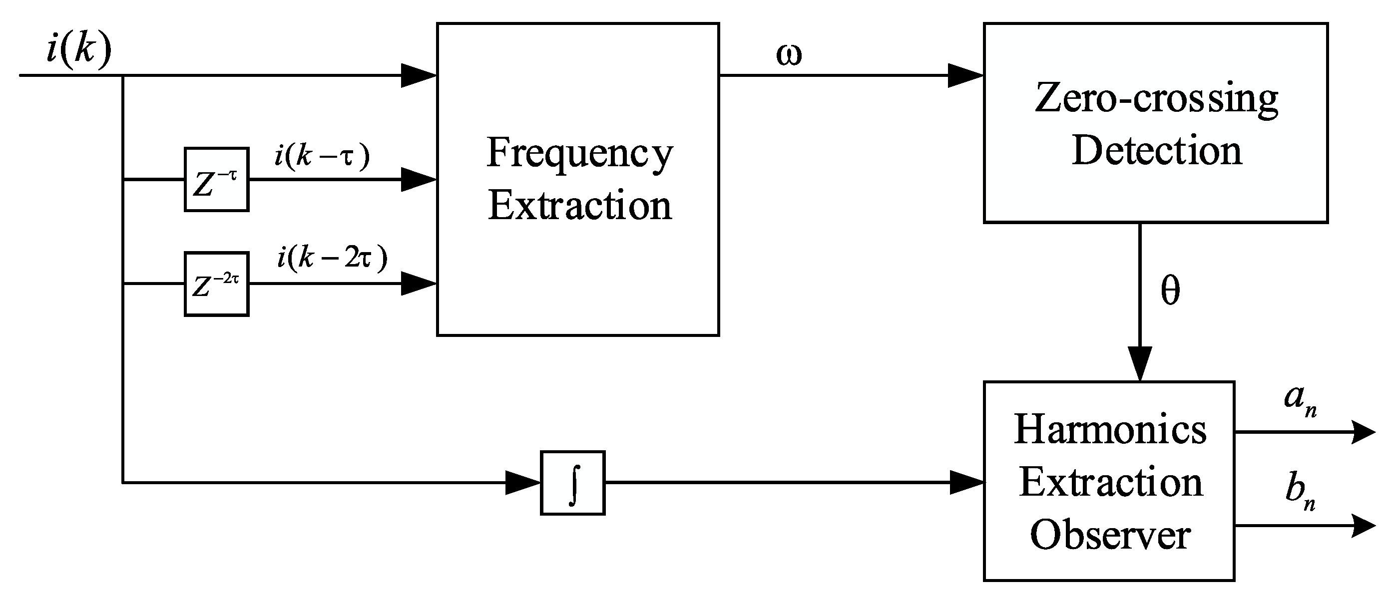
2.1. Robust Frequency Extraction

As mentioned in [29], the real-time tracking of frequencies is achieved using a robust frequency estimation, and a mathematical model is constructed. From Fourier series theory, a periodic current signal involving harmonic disturbances in the power grid can be expressed as [27]

$$i\left(t\right)=A_{1}sin\left(\omega t+{\varphi }_1\right)+\sum _{n=2}^{\infty }{A}_{n}sin\left(n\omega t+{\varphi }_n\right),$$

(1)

where ${\displaystyle \sum _{n=2}^{\infty }}{A}_{n}sin\left(n\omega t+{\varphi }_n\right)$ is the harmonics of $i\left(t\right)$, $\omega$ is angular frequency, t is the time, $A_n$ is amplitude of each harmonic, ${\varphi }_n$ represents the initial phase and n denotes the order of harmonics. By discretizing Formula (1), then using the time delay of the discrete signal, it can be rewritten as

$$i\left(k-\tau \right)=A_{1}sin\left(\omega k{T}_s-\omega \tau +{\varphi }_1\right)+\sum _{n=2}^{\infty }{A}_{n}sin\left(n\omega k{T}_s-n\omega \tau +{\varphi }_n\right),$$

(2)

$$i\left(k-2\tau \right)=A_{1}sin\left(\omega k{T}_s-2\omega \tau +{\varphi }_1\right)+\sum _{n=2}^{\infty }{A}_{n}sin\left(n\omega k{T}_s-2n\omega \tau +{\varphi }_n\right),$$

(3)

where $\tau$ is the delay time, $k=0,1,2,\dots$ and $T_s$ represents the sampling time.

After a series of mathematical transformations, it can be rewritten as

$$\begin{array}{ccc}i\left(k\right)+i\left(k-2\tau \right)\hfill & =& {\displaystyle \sum _{n=2}^{\infty }}{A}_{n}sin(n\omega k{T}_s+{\varphi }_n)+{\displaystyle \sum _{n=2}^{\infty }}{A}_{n}sin\left(n\omega k{T}_s-2n\omega \tau +{\varphi }_n\right)\hfill \\ & & -2cos\omega \tau {\displaystyle \sum _{n=2}^{\infty }}{A}_{n}sin(n\omega k{T}_s-n\omega \tau +{\varphi }_n)+2cos\omega \tau i\left(k-\tau \right).\hfill \end{array}$$

(4)

Let the higher harmonics be $\Delta \left(k\right)$, set time delay signals $i\left(k-\tau \right)$ and $i\left(k-2\tau \right)$ as $i_1\left(k\right)$ and $i_2\left(k\right)$, respectively. It can be obtained that

$$i\left(k\right)+i_2\left(k\right)=2cos\omega \tau i_1\left(k\right)-\Delta \left(k\right).$$

(5)

Let $cos\omega \tau =\gamma$. Once $\gamma$ is estimated when the frequency is under distorted conditions, the calculated value is no longer accurate. Defining $\epsilon \left(k\right)$ as the output error,

$$\begin{array}{c}\epsilon \left(k\right)=2\widehat{\gamma }{i}_1\left(k\right)-i\left(k\right)-i_2\left(k\right)\hfill \\ =2\left(\widehat{\gamma }-\gamma \right)i_1\left(k\right)+\Delta \left(k\right)\hfill \\ =2\tilde{\gamma }{i}_1\left(k\right)+\Delta \left(k\right),\hfill \end{array}$$

(6)

where $\widehat{\gamma }$ is the estimation value of $\gamma$ and $\tilde{\gamma }=\widehat{\gamma }-\gamma$ is error signal of estimation. Here, a robust tracking model is established.

$$\widehat{\gamma }\left(k+1\right)=\widehat{\gamma }\left(k\right)-{\displaystyle \frac{2\Gamma \epsilon \left(k\right)i_1\left(k\right)}{m^2\left(k\right)}}+f\left(k\right),$$

(7)

where $m\left(k\right)=\sqrt{K_a+{\left(2i_1\left(k\right)\right)}^2}$, $\Gamma$ is a preset positive parameter and $f\left(k\right)$ is defined as

$$f\left(k\right)=\left\{\begin{array}{c}-{\sigma }_0\tilde{\gamma }\left(k\right),\left|\tilde{\gamma }\left(k\right)\right|\ge {\gamma }^{*}\hfill \\ 0,\left|\tilde{\gamma }\left(k\right)\right|\le {\gamma }^{*}\hfill \end{array},\right.$$

(8)

where ${\gamma }^{*}$ is greater than or equal to the maximum possible value of $\gamma \left(k\right)$ and ${\sigma }_0$ is greater than zero. This method is robust to the influence of harmonics in non-ideal cases. The structure of the robust extraction method is shown in Figure 2. Therefore, the frequency estimation of power system with higher harmonics can be obtained by

$$\widehat{\omega }\left(k\right)=\frac{arccos\left(\widehat{\gamma }\left(k\right)\right)}{\tau },$$

(9)

where $\widehat{\omega }\left(k\right)$ is the estimation value of true value $\omega \left(k\right)$. The proof of effectiveness [29] and theoretical support [30] of this frequency detection will not be discussed at length here.

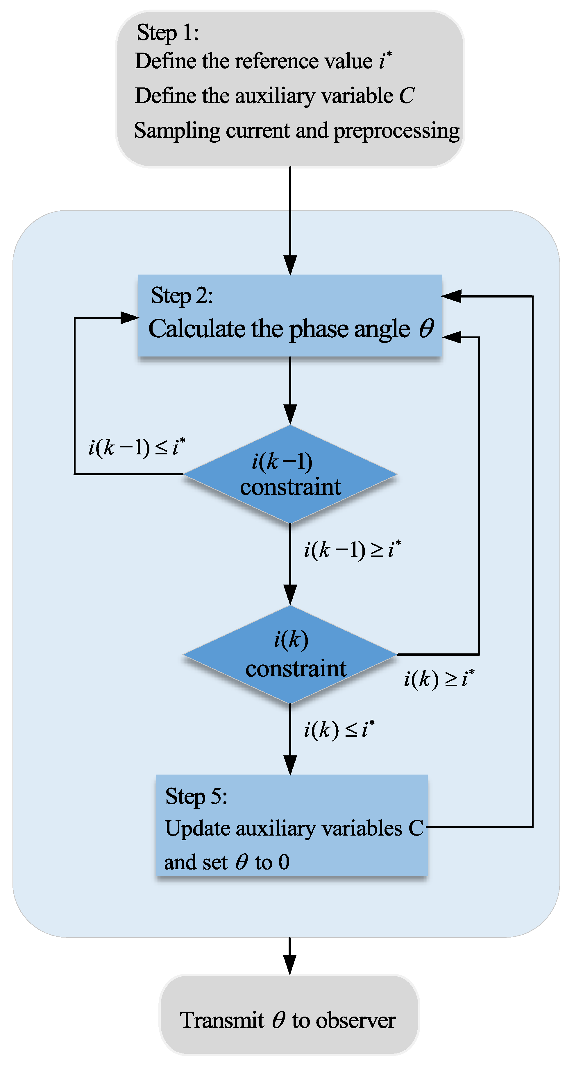
2.2. Zero-Crossing Detection

In this part, the real-time frequency is converted into the phase variable, which is used as the input of the harmonic extraction observer in Section 2.3. The relationship between them follows Formula (10)

$$\theta =\sum \omega \left(k\right)T_s.$$

(10)

Because the existence of errors is inevitable, it will cause the accumulation of errors in the process of phase accumulation. To eliminate the cumulative error, the phase error is cleared at the end of each cycle. The zero-crossing detection algorithm of the current is shown in Figure 3, which illustrates in detail the procedure of the algorithm used to eliminate the cumulative error in the phase angle.

The procedure of the algorithm for each sampling cycle is the same. For the zero-crossing detection here, the aim is to eliminate the errors that occur in each cycle in time, and the method presupposes that the signal being detected has both positive and negative values. If the collected signal does not have the above properties, such problems can be solved by changing the reference value.

• At step 1, the reference $i^{*}$ for the determination is defined, where $i^{*}$ is equal to 0. Furthermore, the auxiliary variable C is defined and its initial value is set to 0. In addition, the signal needs to be sampled and preprocessed.
• At step 2, the phase angle $\theta$ is calculated by $\theta =\theta -C$. After $\theta$ is calculated for the current sampling period, go to step 3 to prepare the phase angle calculation for the next sampling moment.
• At step 3, execute and determine whether $i(k-1)$ at the last sampling moment is greater than $i^{*}$. If $i(k-1)$ is not greater than $i^{*}$, the algorithm continues back to step 2. If the value of $i(k-1)$ is higher than the reference value $i^{*}$, then continue to step 4.
• At step 4, execute and determine whether $i\left(k\right)$ at the current sampling moment is greater than $i^{*}$. If $i\left(k\right)$ is greater than the reference $i^{*}$, the algorithm continues back to step 2. If signal $i\left(k\right)$ is lower than the reference value $i^{*}$, then continue to step 5.
• At step 5, after the determination conditions of both step 3 and step 4 are satisfied, step 5 sets the phase angle $\theta$ to 0 to satisfy the consistency with the phase of the detected signal. Prior to this, the auxiliary variable $C=C+\theta$ is updated.

2.3. Harmonics Extraction Method

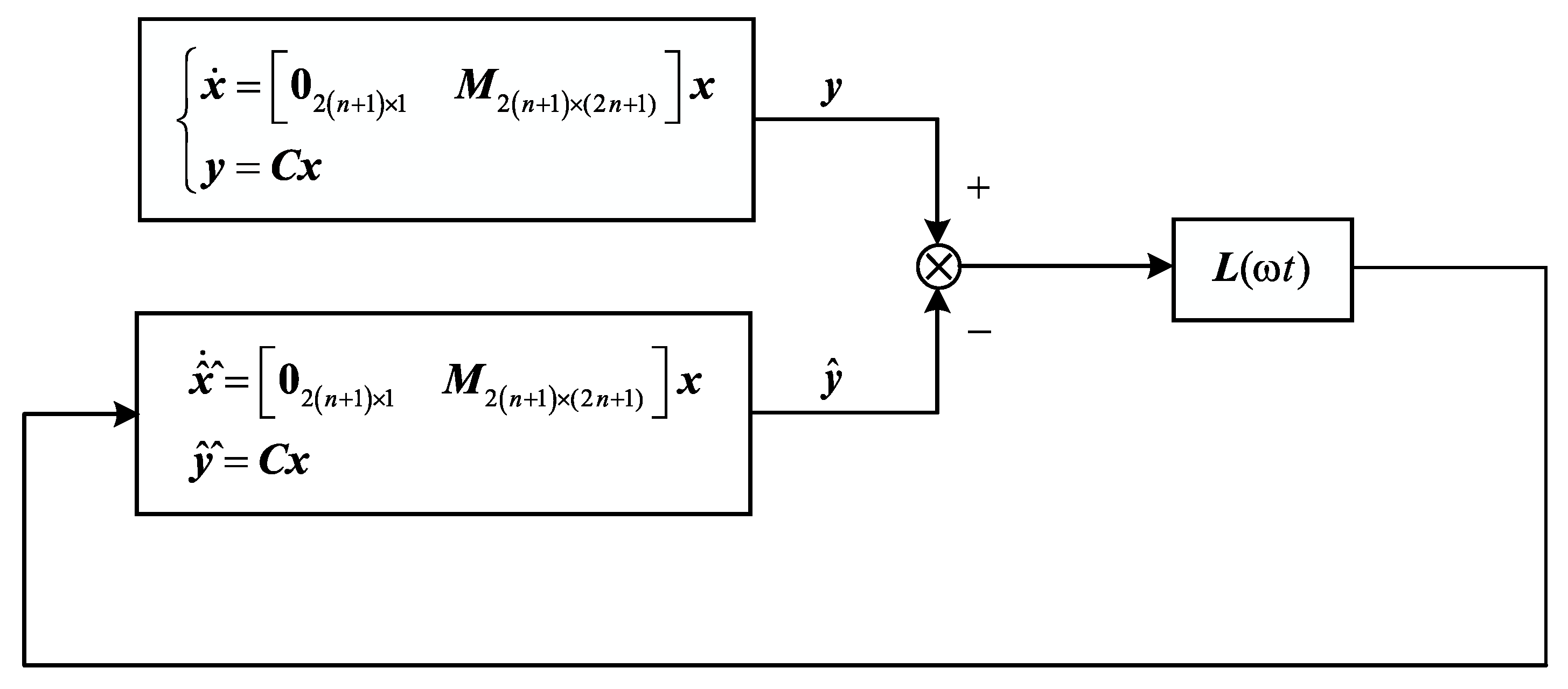
2.3.1. Harmonics Observer Design

According to [31], the grid current expression can be written as

$$i_a\left(t\right)=a_0+\sum a_{n}cos\left(n\theta \right)+b_{n}sin\left(n\theta \right),$$

(11)

where $\theta =\omega t+{\varphi }_1$ represents the phase, $a_0$ is the DC component and ${\varphi }_1$ is the initial phase. Once the values of $\left\{a_0,a_1,b_1,\dots ,a_n,b_n\right\}$ are detected, DC component and harmonics can be obtained directly.

Set $\mathit{x}={[x_1{x}_2{x}_3{x}_4\cdots x_{2n+1}{x}_{2n+2}]}^T={[\int i_a\left(t\right)dt{a}_0{a}_1{a}_2\cdots a_n{b}_n]}^T$ as the state vector, and a dynamic system can be established as

$$\left\{\begin{array}{c}\dot{\mathit{x}}=\left[{\mathbf{0}}_{2(n+1)\times 1}{\mathit{M}}_{2(n+1)\times (2n+1)}\right]\mathit{x}\hfill \\ \mathit{y}=\mathit{Cx}\hfill \end{array}\right.,$$

(12)

where $\mathit{y}$ denotes output vector and

$$\mathit{M}=\left[\begin{array}{cccccc}1\hfill & cos\theta \hfill & \sin \theta \hfill & \cdots \hfill & \cos \left(n\theta \right)\hfill & \sin \left(n\theta \right)\hfill \\ {\mathbf{0}}_{(2n+1)\times (2n+1)}\hfill \end{array}\right],$$

(13)

$$\begin{array}{c}\hfill \mathit{C}={\left[\begin{array}{ccccc}1& 0& 0& \cdots & 0\end{array}\right]}_{1\times 2(n+1)}\end{array}.$$

(14)

Based on Formula (12), a linear time-varying observer is built, and the error feedback is returned back to the observer for continuous correction so that $\widehat{\mathit{x}}$ approximates the true value of $\mathit{x}$. The observer equation is:

$$\left\{\begin{array}{c}\dot{\widehat{\mathit{x}}}=\left[\begin{array}{cc}{0}_{2\left(n+1\right)\times 1}& {\mathit{M}}_{2\left(n+1\right)\times (2n+1)}\end{array}\right]\widehat{\mathit{x}}-\mathit{L}\left(\omega t\right)(\widehat{\mathit{y}}-\mathit{y})\hfill \\ \widehat{\mathit{y}}=\mathit{C}\widehat{\mathit{x}}\hfill \end{array}\right.,$$

(15)

where

$$\mathit{L}\left(\omega t\right)={\left[\begin{array}{ccc}{L}_0& L_{a0}& L_{a1}cos\theta \end{array}\cdots \begin{array}{cc}{L}_{an}cosn\theta & L_{bn}sinn\theta \end{array}\right]}^T.$$

(16)

$\mathit{L}\left(\omega t\right)$ is the error feedback matrix of the output. $L_0,L_{a0},L_{a1},\dots ,L_{an},L_{bn}$ are feedback coefficients, which are positive constants shown in Table 1. The structure of the harmonic extraction observer is shown in Figure 4.

2.3.2. Effectiveness Proof of Observer

To demonstrate observer validity, the error signal $\tilde{\mathit{x}}=\widehat{\mathit{x}}-\mathit{x}$ is defined. (12) and (15) are subtracted, which can be expressed as

$$\begin{array}{c}\dot{\tilde{\mathit{x}}}=\left(\left[\begin{array}{cc}{\mathbf{0}}_{2\left(n+1\right)\times 1}& {\mathit{M}}_{2\left(n+1\right)\times (2n+1)}\end{array}\right]-\mathit{L}\left(\omega t\right)\mathit{C}\right)\tilde{\mathit{x}}=\mathit{H}\tilde{\mathit{x}}.\hfill \end{array}$$

(17)

If it is proved that $\widehat{\mathit{x}}$ converges to $\mathit{x}$ when $t\to \infty$, i.e., $\tilde{\mathit{x}}\to$ 0, it denotes that the estimator of the observer $\widehat{\mathit{x}}$ converges to the actual value $\mathit{x}$. Define the Lyapunov function as

$$V\left(\tilde{\mathit{x}}\right)=\frac{1}{2}{\tilde{\mathit{x}}}^T\mathit{P}\tilde{\mathit{x}},$$

(18)

where $\mathit{P}=diag\left\{1,{\displaystyle \frac{1}{L_{a0}}},{\displaystyle \frac{1}{L_{a1}}},{\displaystyle \frac{1}{L_{b1}}},\dots ,{\displaystyle \frac{1}{L_{an}}},{\displaystyle \frac{1}{L_{bn}}}\right\}$.

Obviously, $V\left(\tilde{\mathit{x}}\right)$ is a positive definite function. Calculate the derivative of $V\left(\tilde{\mathit{x}}\right)$, then

$$\begin{array}{ccc}\hfill \dot{V}\left(\tilde{\mathit{x}}\right)& =& \frac{1}{2}{\dot{\tilde{\mathit{x}}}}^T\mathit{P}\tilde{\mathit{x}}+\frac{1}{2}{\tilde{\mathit{x}}}^T\mathit{P}\dot{\tilde{\mathit{x}}}\hfill \\ \hfill & =& \frac{1}{2}[{\left(\mathit{H}\tilde{\mathit{x}}\right)}^T\mathit{P}\tilde{\mathit{x}}+{\tilde{\mathit{x}}}^T\mathit{P}\left(\mathit{H}\tilde{\mathit{x}}\right)]\hfill \\ \hfill & =& {\tilde{\mathit{x}}}^T\mathit{PH}\tilde{\mathit{x}}\hfill \\ \hfill & =& -L_0{x}_1^2⩽0,\hfill \end{array}$$

(19)

where

$$\mathit{PH}=\left[\begin{array}{ccc}\begin{array}{ccc}-L_0& 1& cos\theta \\ -1& 0& 0\\ -cos\theta & 0& 0\\ -sin\theta & 0& 0\\ ⋮& ⋮& ⋮\\ -cosn\theta & 0& 0\\ -sinn\theta & 0& 0\end{array}& \begin{array}{ccc}sin\theta & \cdots & cosn\theta \\ 0& \cdots & 0\\ 0& \cdots & 0\\ 0& \cdots & 0\\ ⋮& \ddots & ⋮\\ 0& \cdots & 0\\ 0& \cdots & 0\end{array}& \begin{array}{c}sinn\theta \\ 0\\ 0\\ 0\\ ⋮\\ 0\\ 0\end{array}\end{array}\right].$$

(20)

$\dot{V}\left(\tilde{\mathit{x}}\right)$ satisfies the following conditions: (a) $V\left(\tilde{\mathit{x}}\right)$ is a positive definite function and (b) $\dot{V}\left(\tilde{\mathit{x}}\right)\le 0$. Therefore, $V\left(\tilde{\mathit{x}}\right)$ is a Lyapunov function.

In order to prove the convergence of the observer, a set $S\left(r\right)=\left\{\tilde{\mathit{x}}\in {\mathbb{R}}^{2\left(n+1\right)}|V\left(\tilde{\mathit{x}}\right)<r\right\}$ and its largest invariant set $E\left(r\right)=\left\{\tilde{\mathit{x}}\in S\left(r\right)|\dot{V}\left(\tilde{\mathit{x}}\right)=0\right\}$ are defined. It is obviously that any ${\tilde{\mathit{x}}}_E=\left[{\tilde{x}}_{1E}{\tilde{a}}_{0E}{\tilde{a}}_{1E}{\tilde{b}}_{1E}\cdots {\tilde{a}}_{nE}{\tilde{b}}_{nE}\right]\in E\left(r\right)$ always satisfies

$$\begin{array}{c}\hfill \frac{dV\left({\tilde{\mathit{x}}}_E\right)}{dt}=0,\\ \hfill {\tilde{x}}_{1E}=0.\end{array}$$

(21)

From (21), it can be obtained that

$${\tilde{a}}_{0E}+{\tilde{a}}_{1E}cos\theta +{\tilde{b}}_{1E}sin\theta +\cdots +{\tilde{a}}_{nE}cosn\theta +{\tilde{b}}_{nE}sinn\theta =0.$$

(22)

Since $1,cos\theta ,sin\theta ,\dots ,cosn\theta ,sinn\theta$ is linear independent, Equation (22) has only one set of solutions,

$$\left[{\tilde{a}}_{0E}{\tilde{a}}_{1E}{\tilde{b}}_{1E}\cdots {\tilde{a}}_{nE}{\tilde{b}}_{nE}\right]=0.$$

(23)

According to LaSalle’s Invariance Principle, it means that any point in $S\left(r\right)$ converges to 0 as time t tends to infinity, i.e., $\tilde{x}$ converges to 0 when t $\to \infty$.

Discretizing the continuous form of the observer equation, the sampling period is expressed by $T_s$.

$$\left\{\begin{array}{c}{\widehat{x}}_1(k+1)=T_s\left[{\widehat{a}}_0\left(k\right)+{\displaystyle \sum _{n=1}^{\infty }}({\widehat{a}}_{n}cos\left(n\theta \right)+{\widehat{b}}_{n}sin\left(n\theta \right))-L_0({\widehat{x}}_1\left(k\right)-x_1\left(k\right))\right]+{\widehat{x}}_1\left(k\right)\hfill \\ {\widehat{a}}_0(k+1)=-T_s{L}_{a0}({\widehat{x}}_1\left(k\right)-x_1\left(k\right))+{\widehat{a}}_0\left(k\right)\hfill \\ {\widehat{a}}_n(k+1)=-T_s{L}_{an}\cos \left(n\theta \right)({\widehat{x}}_1\left(k\right)-x_1\left(k\right))+{\widehat{a}}_n\left(k\right)\hfill \\ {\widehat{b}}_n(k+1)=-T_s{L}_{bn}\sin \left(n\theta \right)({\widehat{x}}_1\left(k\right)-x_{1}k))+{\widehat{b}}_n\left(k\right)\hfill \end{array}.\right.$$

(24)

3. Simulation

In order to verify the feasibility of the proposed method of extracting harmonics in this study, simulation is carried out in Matlab/Simulink. According to the sampling frequency in [7,11,32], the sampling frequency $f_s$ is set to 40 kHz in simulation. The simulation results will be presented in the later part of this section from different perspectives. Considering that the object under study is the actual distorted grid current, the current signal is set as follows.

$$\begin{array}{cc}\hfill i_a=& 4cos\left(\omega t\right)+2sin\left(\omega t\right)+0.25cos\left(5\omega t\right)+0.3sin\left(5\omega t\right)+0.02cos\left(7\omega t\right)\hfill \\ \hfill & +0.05sin\left(7\omega t\right)+0.0015cos\left(11\omega t\right)+0.0030sin\left(11\omega t\right),\hfill \end{array}$$

(25)

where $\omega =2\pi f$ and f is the grid frequency. The initial value of the grid frequency is designed to be 50 Hz.

The simulation validation provides a complete demonstration of the performance of the proposed method under different scenarios. The following three different scenarios in three dimensions, frequency, phase angle, and amplitude of the signal, are simulated.

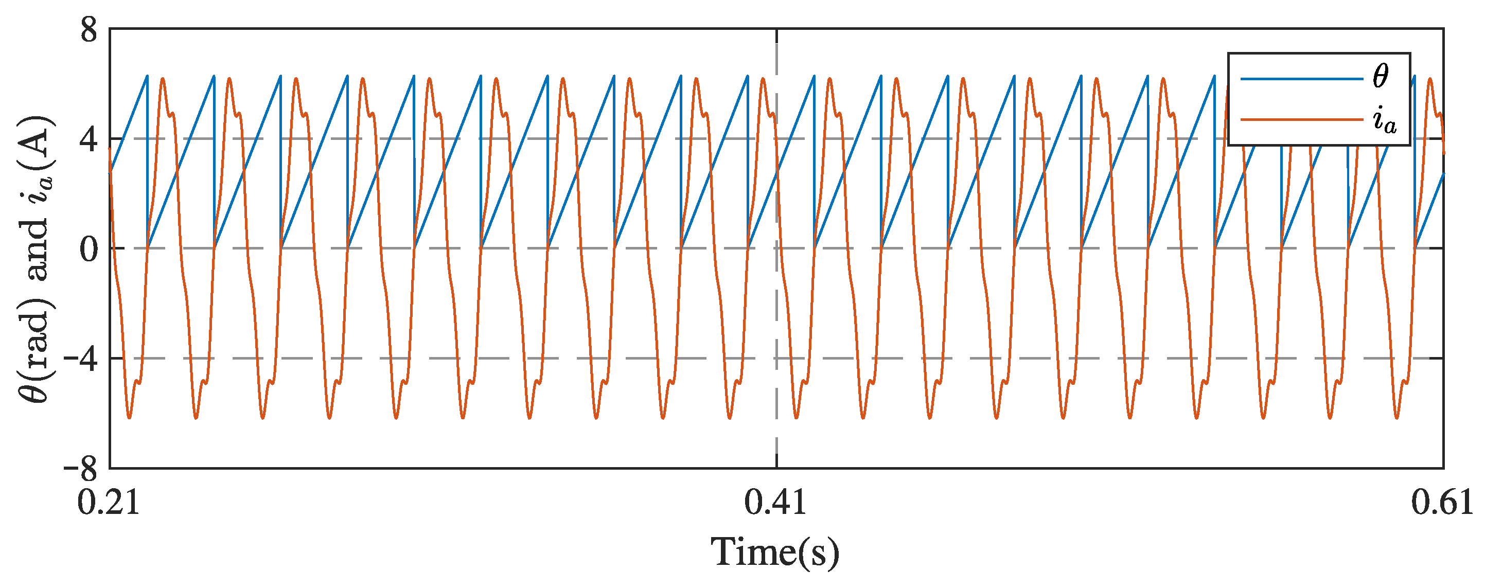
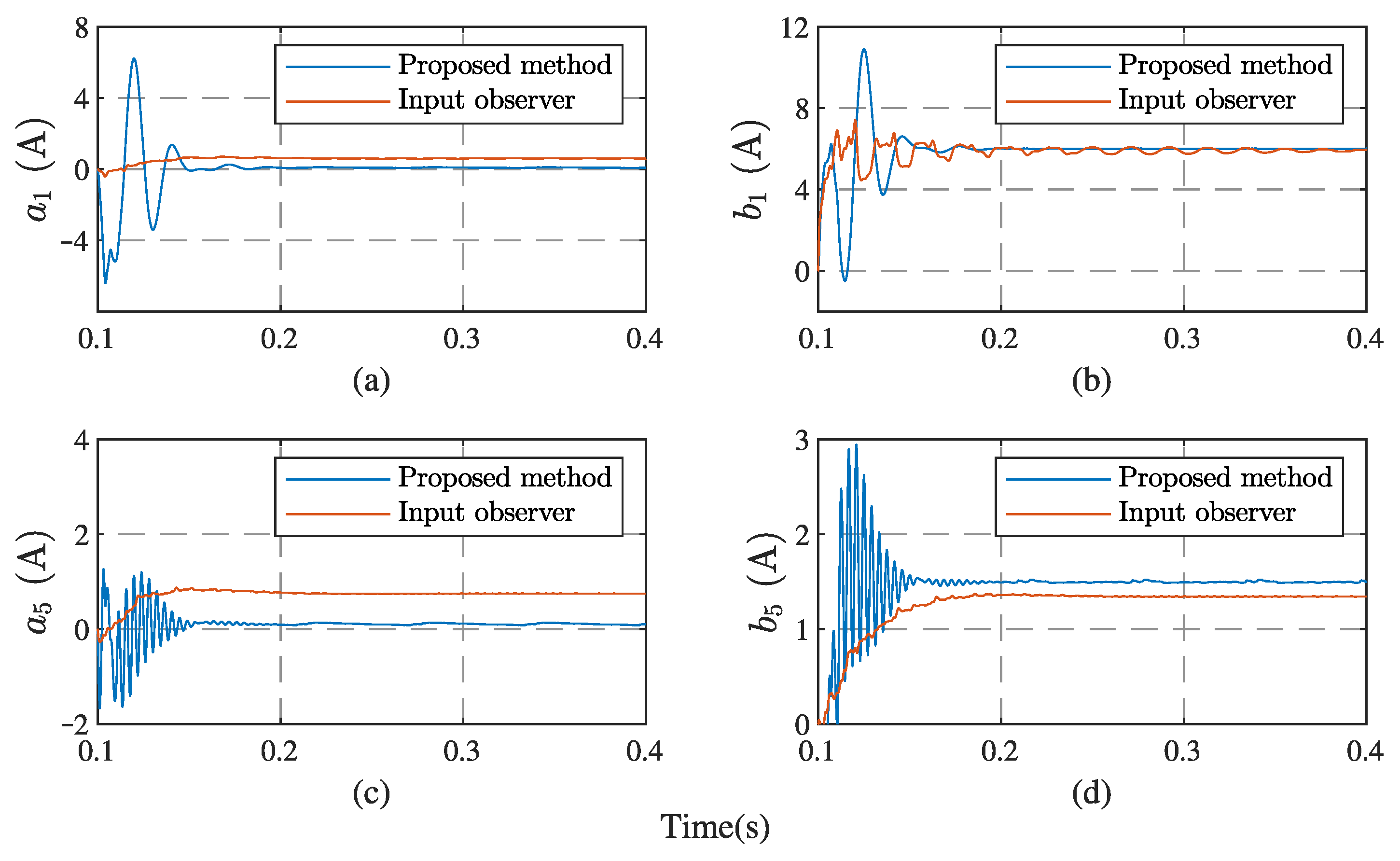
• Case 1: Harmonic extraction of a distorted power grid without any current parameter jump. In this scenario, the feasibility of three parts of harmonic detection can be analyzed and derived, namely frequency estimation, phase angle calculation and harmonic component extraction, respectively.
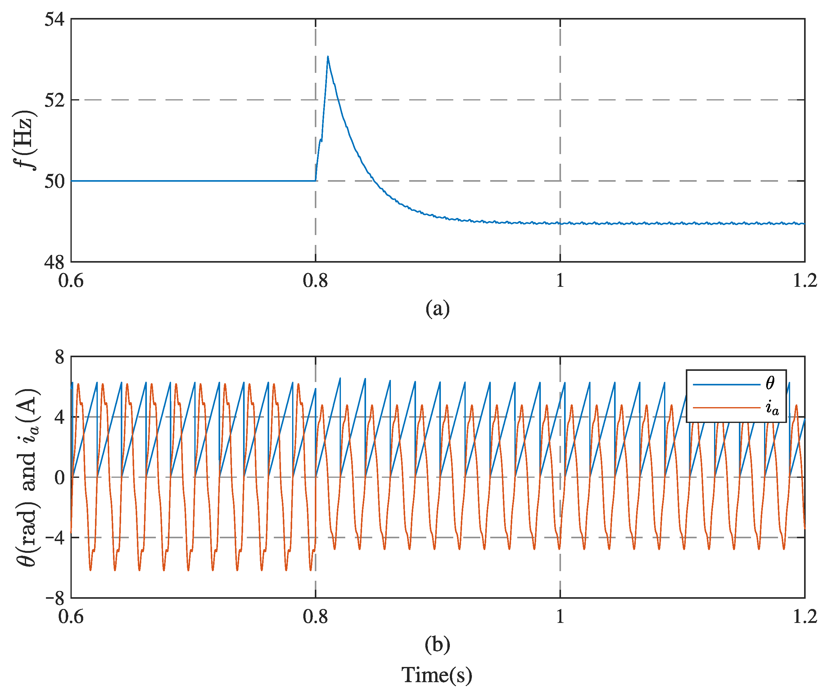
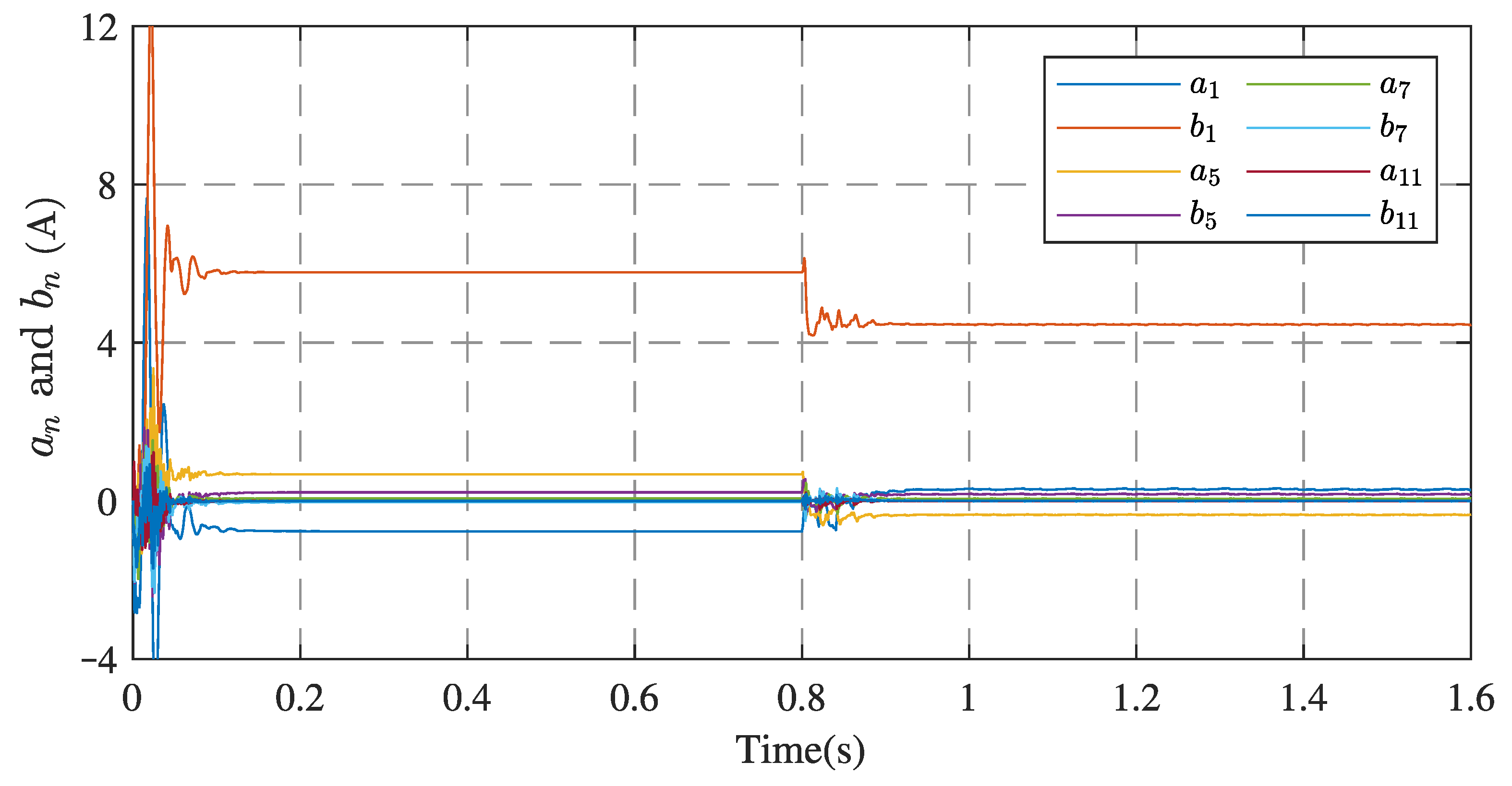
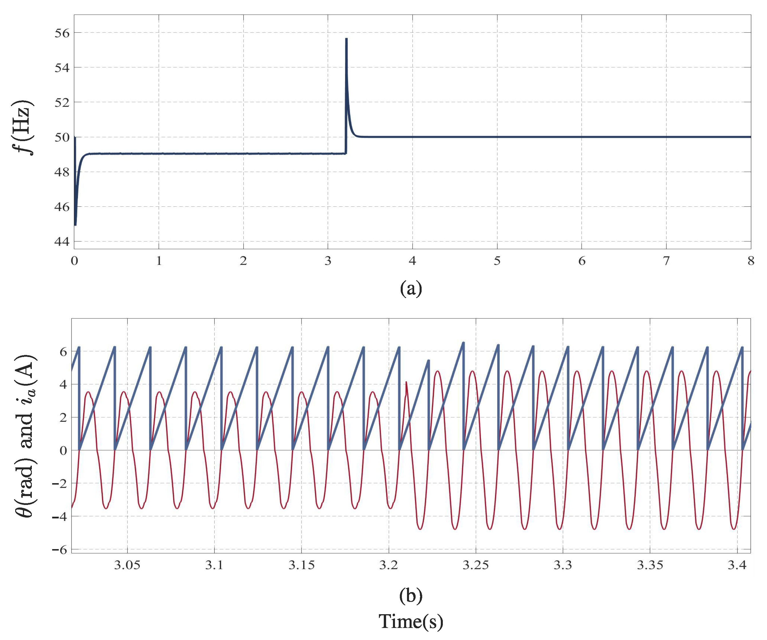
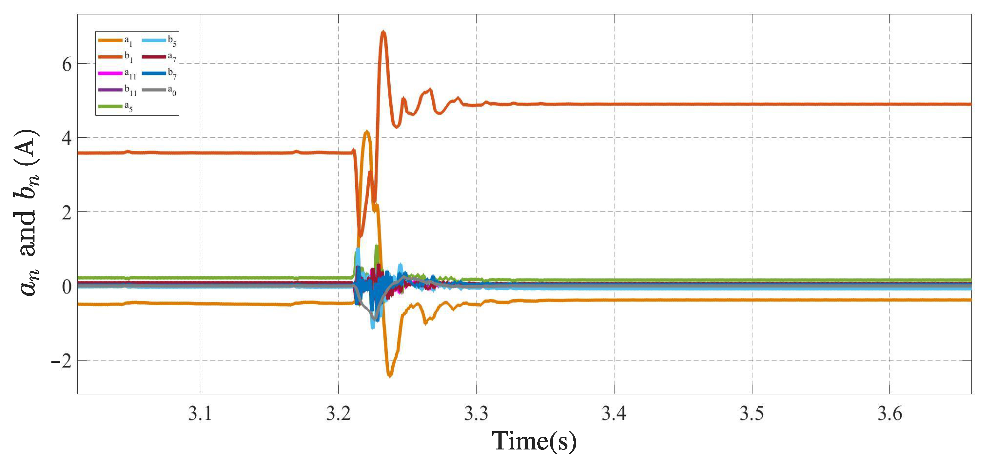
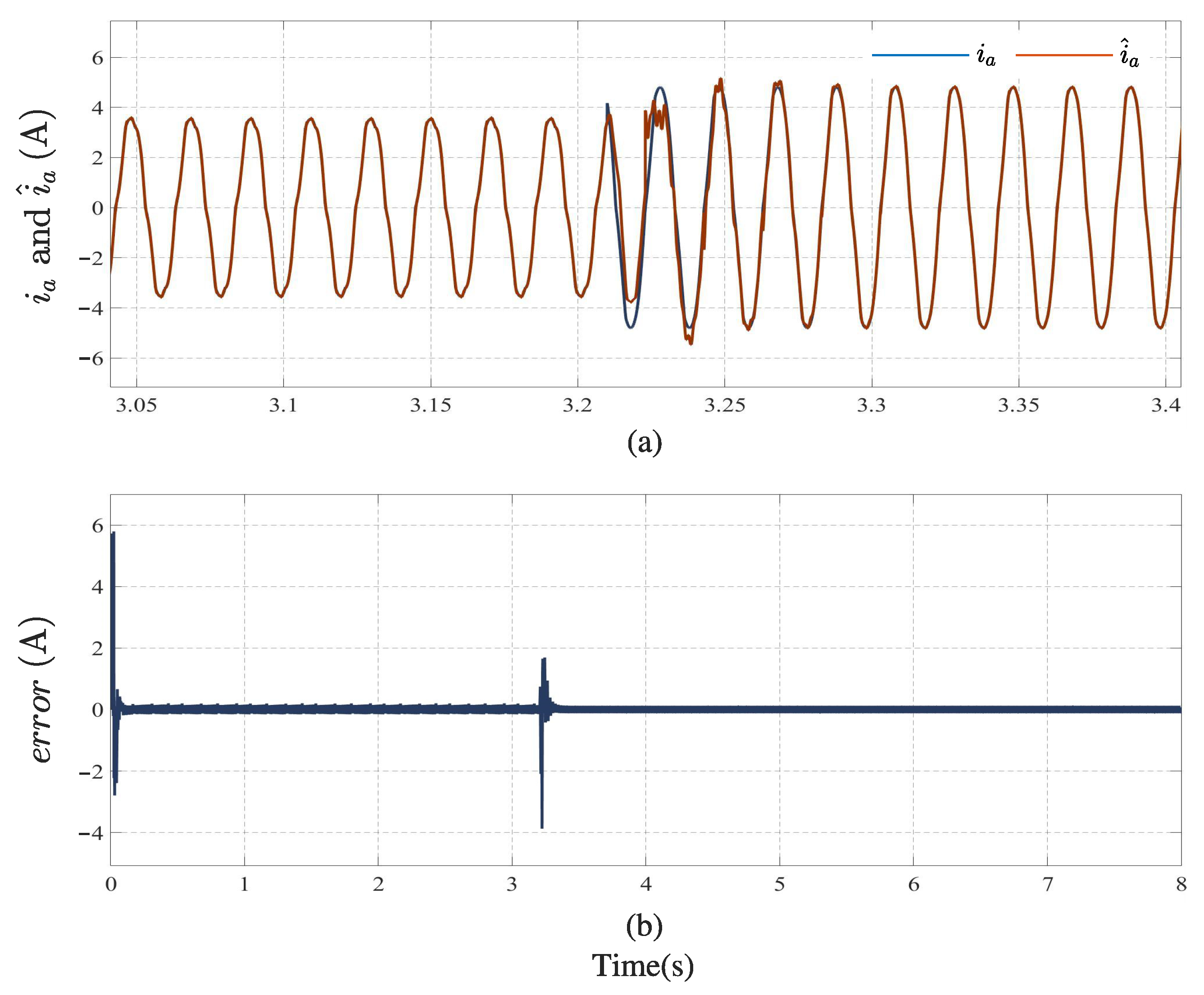
• Case 2: The fundamental frequency and amplitude of the current signal are distorted again. In this scenario, the frequency and the amplitude of the signal jumps at a certain moment, which is a test for the dynamic performance of the proposed method. The specific jump range is given in the following simulation.
• Case 3: The phase angle of the current signal changes abruptly. In this scenario, unlike in the previous case, only the initial phase angle is changed, which leads to deviations from the true value of the phase derived in the zero-crossing detection. In order to provide a more visible picture of the impact of the sudden phase angle change, the phase shift is set to $10\pi /11$.

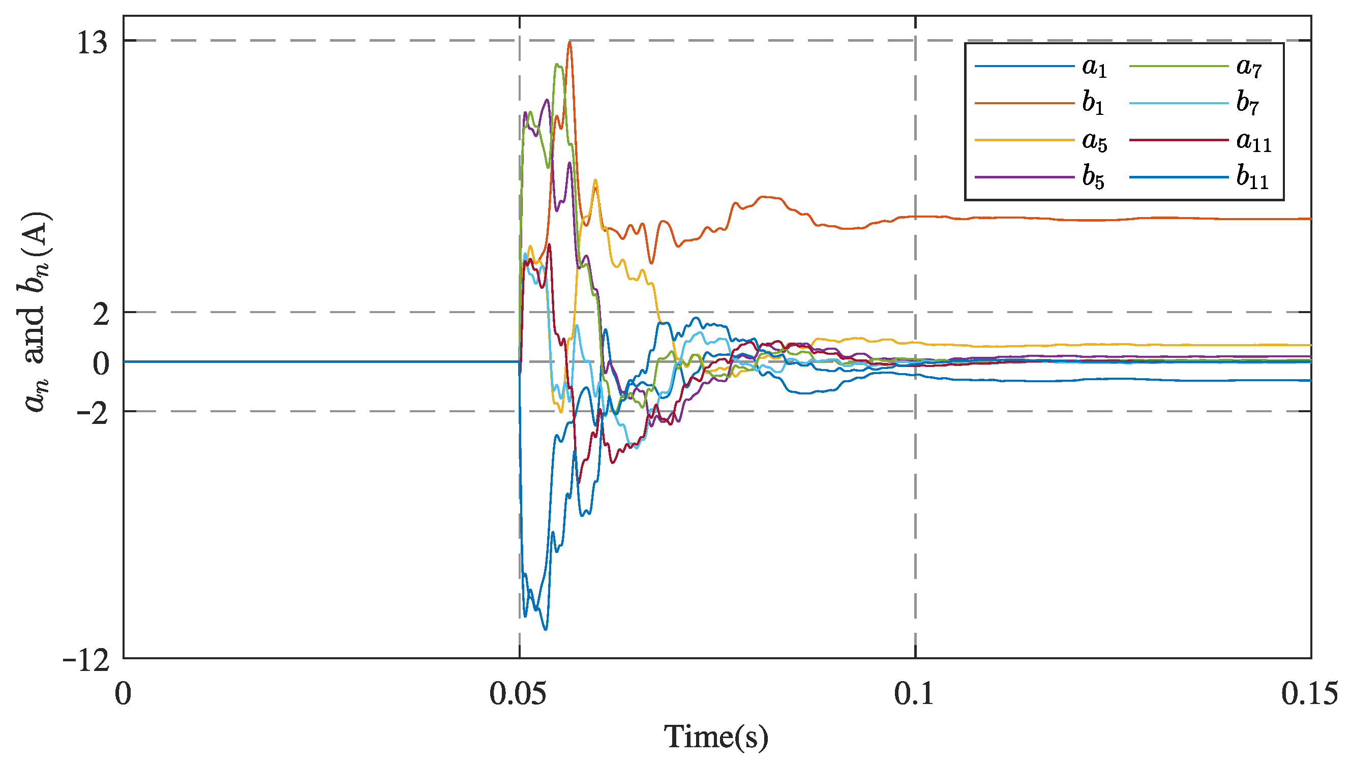
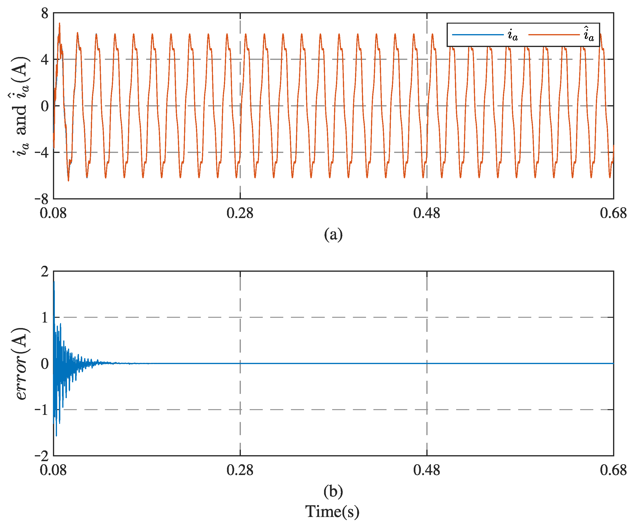
3.1. Verification: Case 1

Regarding Case 1, a current signal identical to Equation (25) is generated in the simulation to simulate the set scenario. Figure 5 shows the simulation results for the feasibility of zero-crossing detection in the proposed method. The result shown in Figure 5 indicates that the phase angle $\theta$ obtained by the zero-crossing detection algorithm is accumulated without error, as shown in the figure, which is highly consistent with the original signal. It can be clearly seen that the grid current signal changes to 0 after each cycle and the phase angle immediately becomes 0 under the action of the zero-crossing detection algorithm.

The stable convergence process of each harmonic component extracted by the observer and the tracking of the reconstructed current are shown in Figure 6 and Figure 7, respectively. The reconstructed current ${\widehat{i}}_a$ is obtained by adding the extracted harmonics and DC component. The stable convergence process of each harmonic parameter extraction from 0 to 0.15 s is shown in Figure 6. In the time period of 0 to 0.05 s, due to the fact that the harmonic extraction algorithm is not introduced, the obtained harmonic parameters are 0. At 0.05 s, the harmonic extraction part is applied. At this time, the harmonics are effectively calculated, but cannot immediately converge to the accurate value. The observer is in a dynamic transition process. At almost 0.1 s, the harmonic parameters gradually tend to be stable. It is clear that each harmonic parameter converges within 80 ms, which means that the algorithm can extract each harmonic component in four cycles. On the premise of an accurate phase angle, the proposed method can extract the information of each harmonic for any signal containing periodic harmonic components. If the frequency and amplitude fluctuation rate of the detected signal are very large, its convergence may be poor. The traditional amplitude phase detection time is more than 80 ms [33], so further harmonic extraction of the signal will take a longer time.

Simulation results of the reconstructed current are shown in Figure 7a, which indicates that ${\widehat{i}}_a$ can track $i_a$ well. The error is defined as an index to characterize the difference between ${\widehat{i}}_a$ and $i_a$. From Figure 7b, the error converges to 0 quickly. It is proved that the original current can be deduced back through the extracted harmonic components, and the correctness of the extraction results and the effectiveness of the harmonic extraction are verified.

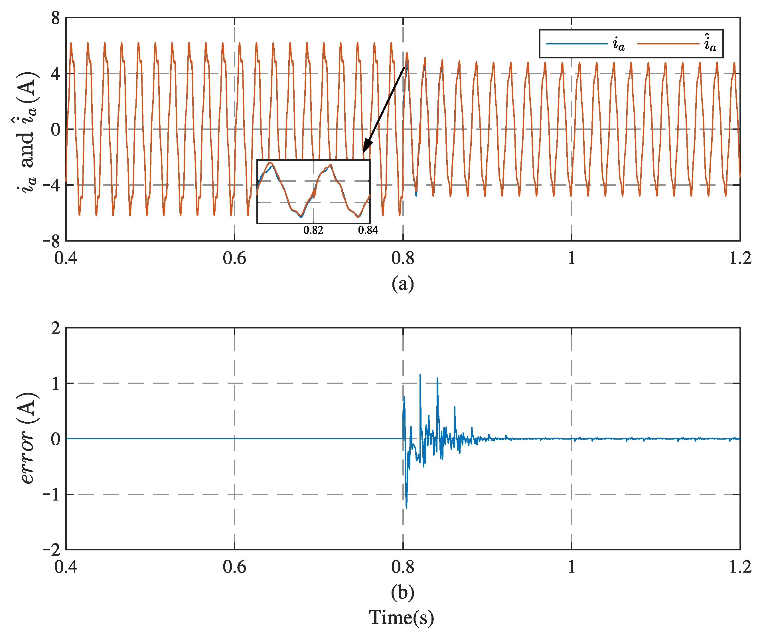
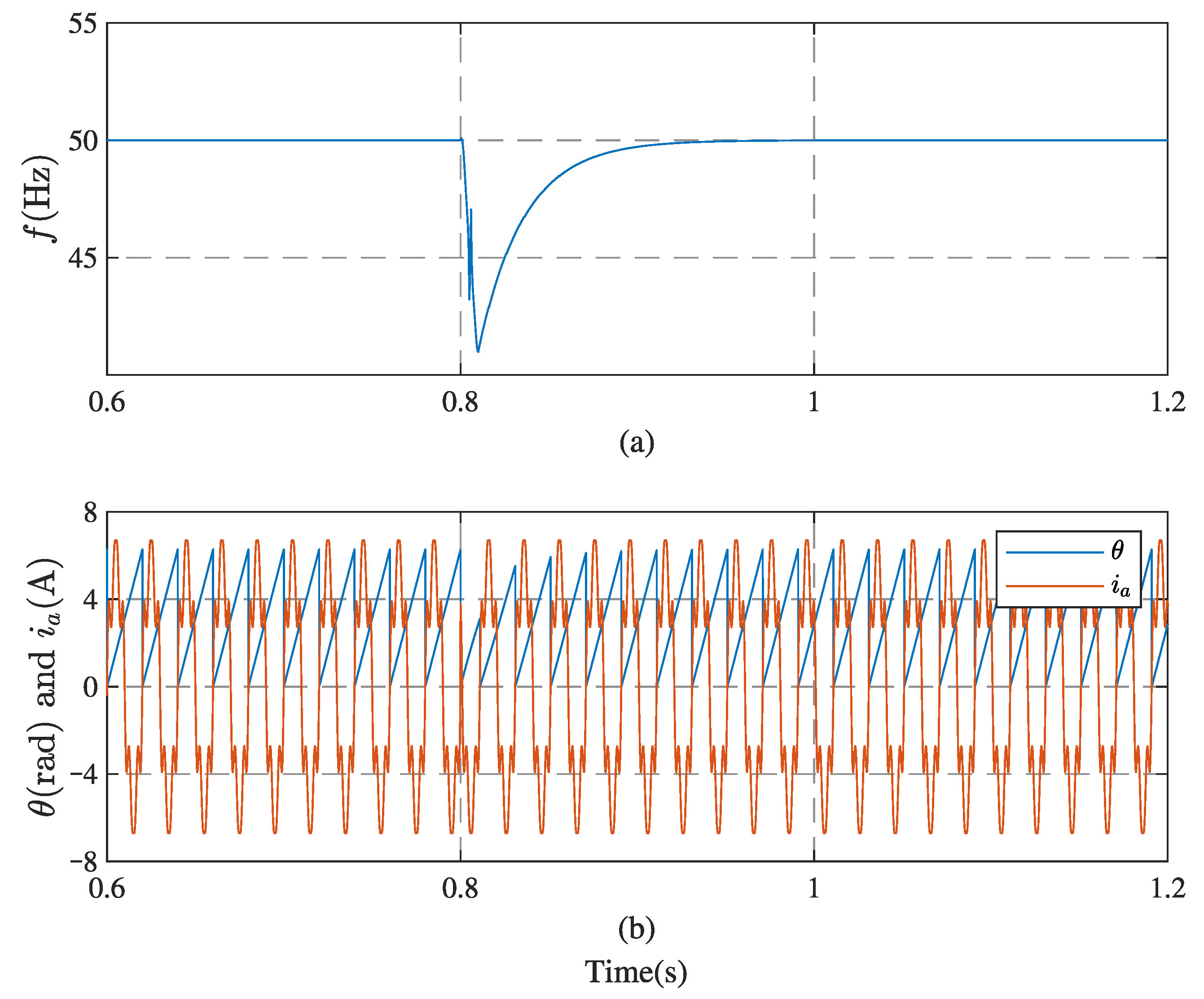
3.2. Verification: Case 2

Considering that the distorted power grid not only contains corresponding harmonics, but may also have frequency or amplitude jumps due to the influence of various factors during normal operation, in order to verify the anti-interference performance of the proposed method, a simulation test with sudden changes in amplitude and frequency is implemented. In this subsection, the expression of the current signal $i_a$ after the jump is as follows:

$$\begin{array}{cc}\hfill i_a=& 3cos\left(\omega t\right)+5sin\left(\omega t\right)+0.5cos\left(5\omega t\right)+0.5sin\left(5\omega t\right)+0.05cos\left(7\omega t\right)\hfill \\ \hfill & +0.05sin\left(7\omega t\right)+0.0015cos\left(11\omega t\right)+0.0030sin\left(11\omega t\right).\hfill \end{array}$$

(26)

The result in Figure 8a shows that the target frequency can be estimated by the proposed method. In this paper, the frequency and amplitude jump times are set at 0.8 s. When the frequency changes from 50 Hz to 49 Hz, it can be obtained that the frequency value of $i_a$ observed by the algorithm immediately jumps upward, so the frequency is quickly re-estimated. From Figure 8b, the changes in the frequency and amplitude occurring at 0.8 s has little effect on zero-crossing detection, and the phase variable $\theta$ is also accurately obtained after the jump occurs.

Figure 9 shows the output harmonic parameters $\left\{a_n,b_n\right\}$ of each order harmonic obtained by the observer. Whether it is the dynamic transition at the beginning or after suffering from the jump, the parameters of harmonic components converge within 80 ms. Using the harmonic component obtained by the proposed algorithm to reconstruct the current, a reconstructed current gradually converging to the original grid current is obtained in Figure 10a. The error current is shown in Figure 10b. As expected, the reconstructed current can also track the original current well. The adjustment time within 80 ms after frequency hopping and amplitude hopping also shows that it can quickly converge to stability.

Based on the simulation results of the error current, one of the main findings is that although the frequency and amplitude jumps at 0.8 s increase the error suddenly to about 1 A, it can be concluded that the proposed algorithm has a good convergence performance. The magnitude of the error can be reduced to almost 0 in less than 80 ms.

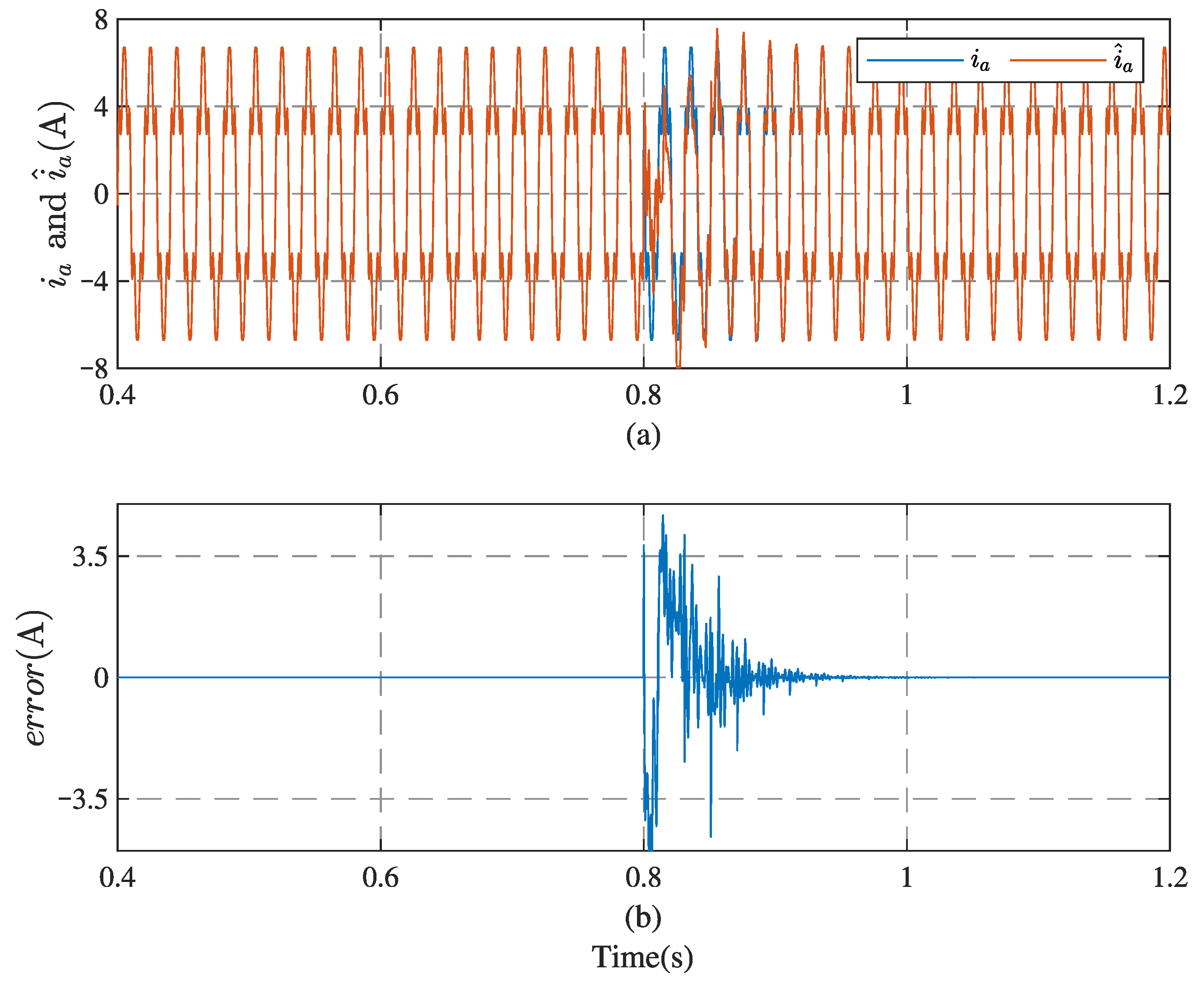
3.3. Verification: Case 3

This subsection will present the scenario described in Case 3 where only the phase changes. The grid current with the parameters is defined as follows:

$$\begin{array}{cc}\hfill i_a=& 6sin\left(\omega t\right)+1.5sin\left(5\omega t\right)+0.7sin\left(7\omega t\right)+0.1sin\left(11\omega t\right),\hfill \end{array}$$

(27)

where the grid frequency is designed to be 50 Hz. To show the effect of the abrupt phase angle change, the phase shift is set to $10\pi /11$ at 0.8 s.

The results of the frequency and phase angle estimation under the condition of abrupt phase change are shown separately in Figure 11. In contrast to Figure 8, it can be concluded that the abrupt phase change of the signal directly affects the frequency estimation as well as the phase detection results. Since the frequency of the original current signal is not changed, the frequency finally returns to its initial value.

Figure 12 shows the extraction of the harmonic component values, and it shows that the abrupt change in phase has some effect on the extraction of the harmonic observer, but does not affect the accurate extraction of each parameter or the convergence of the observer. Similar to Case 2, the reconstructed grid current and the error of the current are shown in Figure 13. Compared with the error shown in Figure 10b, it can be seen that the error current of Case 3 in the dynamic transition stage fluctuates greatly, which is related to the size of the phase shift angle. Changing the phase shift angle is equivalent to translating the original grid current on the coordinate axis; the larger the angle of translation, the larger the corresponding error when the phase jump occurs.

Table 2. Parameters comparison.

n	1	5	7	11
f/Hz	50	250	350	550
$a_n$	0	0	0	0
$b_n$	6.0	1.5	0.7	0.1
${\widehat{a}}_n$	0.07711	0.05889	0.06289	0.01409
${\widehat{b}}_n$	5.99980	1.49880	0.69894	0.09963
$c_n=\sqrt{{a_n}^2+{b_n}^2}$	6.0	1.5	0.7	0.1
${\widehat{c}}_n=\sqrt{{{\widehat{a}}_n}^2+{{\widehat{b}}_n}^2}$	6.00029	1.49996	0.70176	0.10062
$e_{a_n}$	–	–	–	–
$e_{b_n}$	−0.003%	−0.080%	−0.151%	−0.370%
$e_{c_n}$	0.005%	−0.003%	0.251%	0.620%

gives a more complete comparison of the current signal with the harmonic information obtained by the proposed method. In Table 2, $a_n$ and $b_n$ denote the real values, and ${\widehat{a}}_n$ and ${\widehat{b}}_n$ denote the parameter values obtained by the observer where $c_n$ and ${\widehat{c}}_n$ represent the harmonic amplitudes of the real current and the reconstructed current, respectively. $e_{c_n}$ represents the relative error between $c_n$ and ${\widehat{c}}_n$. It can be seen from the table that the relative errors of the 1st, 5th, 7th and 11th harmonics are 0.005%, −0.003%, 0.251% and 0.620%, respectively, and the error is small enough. It is worth noting that the available data are not considered to be subject to uncertainty or inaccuracy. As for such problems, fuzzy logic [34,35,36] may bring better results.

Table 1. System and control parameters.

${\mathit{\sigma }}_0$	$\mathbf{\Gamma }$	${\mathit{L}}_0$	${\mathit{L}}_{\mathit{an}}$	${\mathit{L}}_{\mathit{bn}}$	${\mathit{f}}_{\mathit{s}}$	${\mathit{f}}_{\mathit{c}}$
1/1000	1/1000	1800	1,000,000	1,000,000	40 kHz	40 kHz

Table 1. System and control parameters.

${\mathit{\sigma }}_0$	$\mathbf{\Gamma }$	${\mathit{L}}_0$	${\mathit{L}}_{\mathit{an}}$	${\mathit{L}}_{\mathit{bn}}$	${\mathit{f}}_{\mathit{s}}$	${\mathit{f}}_{\mathit{c}}$
1/1000	1/1000	1800	1,000,000	1,000,000	40 kHz	40 kHz

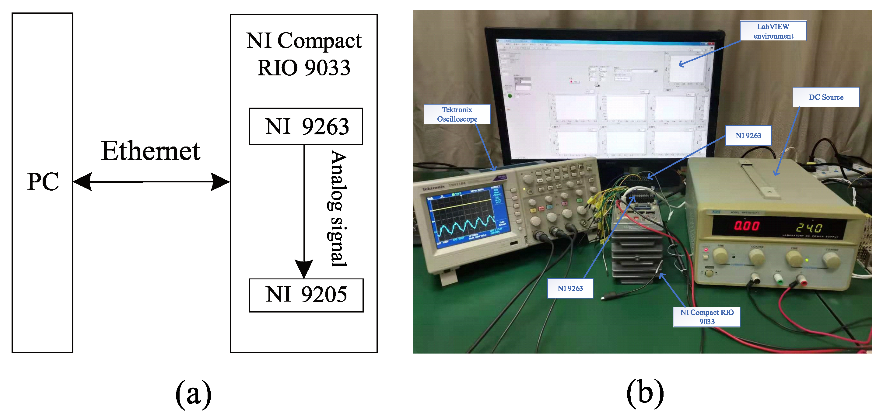
4. Experimental Evaluation

To further validate the effectiveness of the proposed harmonic detection method, an experimental evaluation is carried out on the test platform shown in Figure 14. The platform mainly consists of NI CompactRIO-9033 and LabVIEW software. The key part of the experimental platform is NI CompactRIO-9033, which is a high-speed controller with an embedded FPGA module chip. It can be connected to NI 9025 (analog input module) and NI 9263 (analog output module) through specific ports to transfer data through an internal bus. The LabVIEW environment can realize human–computer interaction, and it can not only upload experimental data to a PC through an Ethernet port, but also make real-time changes during the experiment.

The experiment is similar to the simulation. The whole process is as follows: (1) the proposed algorithm is programmed to the FGPA module in the LabVIEW environment. (2) NI 9205 is used to collect the analog current generated by NI 9263 and pass the signal into the controller NI CompactRIO-9033. (3) The compiled program processes the incoming data to obtain harmonic information. (4) The experimental data are uploaded to the PC. It mainly verifies whether the three parts of the algorithm meet the following requirements: the tracking of frequency, the effectiveness of zero-crossing detection and the convergence of each harmonic extraction result. The system and control parameters are given in Table 1; the sampling frequency of the signal $f_s$ is 40 kHz and the sampling frequency of the controller $f_c$ is also set to 40 kHz.

Figure 15 shows the experimental results after the simultaneous jump of frequency and amplitude. Although the instantaneous fluctuation caused by the jump is greater than the simulation results, it can be seen that the results shown in Figure 15a,b are basically consistent with the simulation results in Section 3.

Figure 16 shows the convergence process of harmonic component parameters from 3.0 s to 3.7 s; it is clear that the parameters can be estimated within a short time.

Figure 17a,b show the tracking of the reconstructed current for the original current signal and the error current between the two, respectively. In short, the results for harmonic components and reconstructed currents demonstrate the accuracy and stability of the observer. It is able to extract harmonics quickly and accurately in the presence of grid frequency and amplitude jumps.

In summary, the experimental results also prove that the proposed method can track the frequency in real time and accurately extract the harmonic components under distortion conditions.

5. Discussion

From the perspective of the results obtained, the proposed harmonic extraction method is able to meet the expected requirements. The frequency estimation algorithm can enable the observer to obtain frequency information when the fundamental frequency of the detected signal is unknown, thus enabling the designed observer to effectively extract each harmonic component.

For the harmonic extraction of the current signal $i_a=6sin(2\pi t\times 48)+1.5sin(5\times 2\pi t\times 48)+0.7sin(7\times 2\pi t\times 48)+0.1sin(11\times 2\pi t\times 48)$, the comparison of this method with the input observer [22] and FFT is shown in the subsequent part.

Table 3. Comparison of methods for harmonic estimation.

n	f/Hz	FFT	Proposed Method			True Value
		Mag (A)	${\widehat{\mathit{a}}}_{\mathit{n}}$	${\widehat{\mathit{b}}}_{\mathit{n}}$	${\widehat{\mathit{c}}}_{\mathit{n}}=\sqrt{{{\widehat{\mathit{a}}}_{\mathit{n}}}^2+{{\widehat{\mathit{b}}}_{\mathit{n}}}^2}$	Mag (A)
1	48	5.999	0.0872	6.0011	6.0017	6.0
5	240	1.501	0.1100	1.4973	1.5013	1.5
7	336	0.6984	0.0727	0.7018	0.7055	0.7
11	528	0.1003	0.0151	0.1012	0.1023	0.1

presents the comparison between the FFT and the method proposed in this paper. The FFT extraction results are obtained by the FFT analysis module of Matleb/Simulink, where $Mag$ represents the amplitude. From Table 3, it can be obtained that the proposed method is not much worse than the FFT method in terms of accuracy. For FFT, however, it is not possible to extract harmonics in real time because it needs to sample at least one cycle of the signal. Of course, it can be inferred that the accuracy of the proposed method decreases as the harmonic order increases, while the FFT does not.

A comparison between the proposed method and the input observer method is shown in Figure 18, which represents the dynamic transition process and steady-state process of the extraction of harmonic components $a_1$, $b_1$, $a_5$ and $b_5$. At 0.1 s, the harmonic extraction algorithm is added. The four subplots (a), (b), (c) and (d) demonstrate that the results obtained by both methods can converge to a certain value in a very short time (a few cycles), and it can be seen from (c) and (d) that the results of the proposed method are closer to the true values of $a_n$ and $b_n$ in terms of the extracted accuracy. In order to present the extraction effect of the first and fifth harmonics more visually, Figure 19 shows the comparison of the harmonic waveforms, where $i_1$ and $i_5$ represent the fundamental wave and fifth harmonic, respectively. The figure shows that the estimates produced by both methods are approximately equivalent after 0.146 s. From both subplots, it can be concluded that the proposed method is advantageous due to it taking less time in the dynamic transition process.

6. Conclusions

In this study, a method for real-time harmonic extraction of distorted grid currents is proposed, which consists of three parts: robust frequency extraction, zero-crossing detection and harmonic parameter extraction. The original current signal is reconstructed by summing the extracted harmonics. Simulations and experiments are performed to verify the effectiveness of the proposed harmonic detection method. Both simulation and experimental results show that the method is able to extract each harmonic quickly and accurately based on the observer and also has good performance in the case of sudden current changes.

The proposed harmonic detection method is accurate and fast. It can extract harmonics effectively and accurately in real time. However, in the process of harmonic extraction, the amplitude jitter is a little large and the transition time is not short enough before obtaining the accurate value of each harmonic parameter. This will be a problem to be solved in future research directions. In addition, the application of harmonic extraction in practice may also be a future work direction, such as transformers, induction motors, etc.

References

1. Cortajarena, J.A.; Barambones, O.; Alkorta, P.; Cortajarena, J. Grid Frequency and Amplitude Control Using DFIG Wind Turbines in a Smart Grid. Mathematics 2021, 9, 143. [Google Scholar] [CrossRef]
2. Shademan, M.; Jalilian, A.; Savaghebi, M. Improved Control Method for Voltage Regulation and Harmonic Mitigation Using Electric Spring. Sustainability 2021, 13, 4523. [Google Scholar] [CrossRef]
3. Zhang, X.; Wang, R.; Bao, J. A Novel Distributed Economic Model Predictive Control Approach for Building Air-Conditioning Systems in Microgrids. Mathematics 2018, 6, 60. [Google Scholar] [CrossRef] [Green Version]
4. Hashempour, M.M.; Savaghebi, M.; Vasquez, J.C.; Guerrero, J.M. A Control Architecture to Coordinate Distributed Generators and Active Power Filters Coexisting in a Microgrid. IEEE Trans. Smart Grid 2016, 7, 2325–2336. [Google Scholar] [CrossRef] [Green Version]
5. Munir, H.M.; Zou, J.; Xie, C.; Guerrero, J.M. Cooperation of Voltage Controlled Active Power Filter with Grid-Connected DGs in Microgrid. Sustainability 2019, 11, 154. [Google Scholar] [CrossRef] [Green Version]
6. Sharma, A.; Rajpurohit, B.S.; Singh, S.N. A review on economics of power quality: Impact, assessment and mitigation. Renew. Sustain. Energy Rev. 2018, 88, 363–372. [Google Scholar] [CrossRef]
7. Selvajyothi, K.; Janakiraman, P.A. Extraction of Harmonics Using Composite Observers. IEEE Trans. Power Deliv. 2008, 23, 31–40. [Google Scholar] [CrossRef]
8. Terriche, Y.; Golestan, S.; Guerrero, J.M.; Kerdoune, D.; Vasquez, J.C. Matrix pencil method based reference current generation for shuntactive power filters. IET Power Electron. 2018, 11, 772–780. [Google Scholar] [CrossRef] [Green Version]
9. Sinvula, R.; Abo-Al-Ez, K.M.; Kahn, M.T. Harmonic Source Detection Methods: A Systematic Literature Review. IEEE Access 2019, 7, 74283–74299. [Google Scholar] [CrossRef]
10. Masoum, A.S.; Hashemnia, N.; Abu-Siada, A.; Masoum, M.A.S.; Islam, S.M. Online Transformer Internal Fault Detection Based on Instantaneous Voltage and Current Measurements Considering Impact of Harmonics. IEEE Trans. Power Deliv. 2017, 32, 587–598. [Google Scholar] [CrossRef]
11. Sapena-Baño, A.; Pineda-Sanchez, M.; Puche-Panadero, R.; Perez-Cruz, J.; Roger-Folch, J.; Riera-Guasp, M.; Martinez-Roman, J. Harmonic Order Tracking Analysis: A Novel Method for Fault Diagnosis in Induction Machines. IEEE Trans. Energy Convers. 2015, 30, 833–841. [Google Scholar] [CrossRef] [Green Version]
12. Ahmad, M.W.; Gorla, N.B.Y.; Malik, H.; Panda, S.K. A Fault Diagnosis and Postfault Reconfiguration Scheme for Interleaved Boost Converter in PV-Based System. IEEE Trans. Power Electron. 2021, 36, 3769–3780. [Google Scholar] [CrossRef]
13. Vardar, K.; Akpınar, E.; Sürgevil, T. Evaluation of reference current extraction methods for DSP implementation in active power filters. Electr. Power Syst. Res. 2009, 79, 1342–1352. [Google Scholar] [CrossRef]
14. Rechka, S.; Ngandui, E.; Xu, J.; Sicard, P. A comparative study of harmonic detection algorithms for active filters and hybrid active filters. In Proceedings of the IEEE 33rd Annual IEEE Power Electronics Specialists Conference, Cairns, QLD, Australia, 23–27 June 2002; pp. 357–363. [Google Scholar]
15. Liu, H.; Hu, H.; Chen, H.; Zhang, L.; Xing, Y. Fast and Flexible Selective Harmonic Extraction Methods Based on the Generalized Discrete Fourier Transform. IEEE Trans. Power Electron. 2018, 33, 3484–3496. [Google Scholar] [CrossRef]
16. Barros, J.; Diego, R.I. Analysis of Harmonics in Power Systems Using the Wavelet Packet Transform. In Proceedings of the IEEE Instrumentationand Measurement Technology Conference, Ottawa, ON, Canada, 16–19 May 2005; pp. 1484–1488. [Google Scholar]
17. Wang, G.; Wang, X.; Zhao, C. An Iterative Hybrid Harmonics Detection Method Based on Discrete Wavelet Transform and Bartlett–Hann Window. Appl. Sci. 2020, 10, 3922. [Google Scholar] [CrossRef]
18. Harirchi, F.; Simões, M.G. Enhanced Instantaneous Power Theory Decomposition for Power Quality Smart Converter Applications. IEEE Trans. Power Electron. 2018, 33, 9344–9359. [Google Scholar] [CrossRef]
19. Bagheri, A.; Mardaneh, M.; Rajaei, A.; Rahideh, A. Detection of Grid Voltage Fundamental and Harmonic Components Using Kalman Filter and Generalized Averaging Method. IEEE Trans. Power Electron. 2016, 31, 1064–1073. [Google Scholar] [CrossRef]
20. Uz-Logoglu, E.; Salor, O.; Ermis, M. Online Characterization of Interharmonics and Harmonics of AC Electric Arc Furnaces by Multiple Synchronous Reference Frame Analysis. IEEE Trans. Ind. Appl. 2016, 52, 2673–2683. [Google Scholar] [CrossRef]
21. Xie, C.; Li, K.; Zou, J.; Zhou, K.; Guerrero, J.M. Multiple Second-Order Generalized Integrators Based Comb Filter for Fast Selective Harmonic Extraction. In Proceedings of the 2019 IEEE Applied Power Electronics Conference and Exposition (APEC), Anaheim, CA, USA, 17–21 March 2019; pp. 2427–2432. [Google Scholar] [CrossRef] [Green Version]
22. Li, P.; Jin, W.; Li, R.; Guan, M. Harmonics detection via input observer with grid frequency fluctuation. Int. J. Electr. Power Energy Syst. 2020, 115, 105461. [Google Scholar] [CrossRef]
23. Xiao, P.; Corzine, K.A.; Venayagamoorthy, G.K. Multiple Reference Frame-Based Control of Three-Phase PWM Boost Rectifiers under Unbalanced and Distorted Input Conditions. IEEE Trans. Power Electron. 2008, 23, 2006–2017. [Google Scholar] [CrossRef]
24. Lai, L.L.; Chan, W.L.; Tse, C.T.; So, A.T.P. Real-time frequency and harmonic evaluation using artificial neural networks. IEEE Trans. Power Deliv. 1999, 14, 52–59. [Google Scholar] [CrossRef]
25. Chang, G.W.; Chen, C.; Teng, Y. Radial-Basis-Function-Based Neural Network for Harmonic Detection. IEEE Trans. Ind. Electron. 2010, 57, 2171–2179. [Google Scholar] [CrossRef]
26. Ujile, A.; Ding, Z. A dynamic approach to identification of multiple harmonic sources in power distribution systems. Int. J. Electr. Power Energy Syst. 2016, 81, 175–183. [Google Scholar] [CrossRef]
27. Ujile, A.; Ding, Z.; Li, H. An iterative observer approach to harmonic estimation for multiple measurements in power distribution systems. Trans. Inst. Meas. Control 2017, 39, 599–610. [Google Scholar] [CrossRef]
28. Samadaei, E.; Iranian, M.; Rezanejad, M.; Godina, R.; Pouresmaeil, E. Single-Phase Active Power Harmonics Filter by Op-Amp Circuits and Power Electronics Devices. Sustainability 2018, 10, 4406. [Google Scholar] [CrossRef] [Green Version]
29. Dai, Z.; Fan, M.; Nie, H.; Zhang, J.; Li, J. A Robust Frequency Estimation Method for Aircraft Grids Under Distorted Conditions. IEEE Trans. Ind. Electron. 2020, 67, 4254–4258. [Google Scholar] [CrossRef]
30. Jiang, Z.P.; Wang, Y. Input-to-state stability for discrete-time nonlinear systems. Automatica 2001, 37, 857–869. [Google Scholar] [CrossRef]
31. Wang, Y.F.; Li, Y.W. A Grid Fundamental and Harmonic Component Detection Method for Single-Phase Systems. IEEE Trans. Power Electron. 2013, 28, 2204–2213. [Google Scholar] [CrossRef]
32. Zhuo, S.; Xu, L.; Gaillard, A.; Huangfu, Y.; Gao, F. Robust Open-Circuit Fault Diagnosis of Multi-Phase Floating Interleaved DC–DC Boost Converter Based on Sliding Mode Observer. IEEE Trans. Transp. Electrif. 2019, 5, 638–649. [Google Scholar] [CrossRef]
33. Xiong, L.; Liu, X.; Liu, L.; Liu, Y. Amplitude-Phase Detection for Power Converters Tied to Unbalanced Grids with Large X/R Ratios. IEEE Trans. Power Electron. 2021. [Google Scholar] [CrossRef]
34. Cacciola, M.; Pellicanò, D.; Megali, G.; Lay-Ekuakille, A.; Versaci, M.; Morabito, F.C. Aspects about air pollution prediction on urban environment. In Proceedings of the 4th IMEKO TC19 Symposium on Environmental Instrumentation and Measurements 2013: Protection Environment, Climate Changes and Pollution Control, Lecce, Italy, 3–4 June 2013. [Google Scholar]
35. Qu, Y.; Tan, W.; Dong, Y.; Yang, Y. Harmonic detection using fuzzy LMS algorithm for active power filter. In Proceedings of the 2007 International Power Engineering Conference (IPEC 2007), Singapore, 3–6 December 2007; pp. 1065–1069. [Google Scholar]
36. Xie, Q.; Ni, J.; Su, Z. A prediction model of ammonia emission from a fattening pig room based on the indoor concentration using adaptive neuro fuzzy inference system. J. Hazard. Mater. 2017, 325, 301–309. [Google Scholar] [CrossRef] [PubMed]
Figure 1. Block diagram of harmonics detection.
Mathematics 09 02245 g001
Figure 2. Block diagram of the robust frequency estimation.
Mathematics 09 02245 g002
Figure 3. Steps of zero-crossing detection algorithm.
Mathematics 09 02245 g003
Figure 4. Block diagram of the harmonic extraction observer.
Mathematics 09 02245 g004
Figure 5. Simulation results of comparison between θ and i a .
Mathematics 09 02245 g005
Figure 6. The stable convergence process of each harmonic parameter extraction.
Mathematics 09 02245 g006
Figure 7. (a) Comparison between reconstructed current i ^ a and original current i a . (b) Error current.
Mathematics 09 02245 g007
Figure 8. Simulation results with frequency and amplitude jump: (a) frequency, (b) comparison between θ and i a .
Mathematics 09 02245 g008
Figure 9. The values of each harmonic parameter extraction with frequency and amplitude jump.
Mathematics 09 02245 g009
Figure 10. (a) Comparison between i ^ a and i a . (b) Error current.
Mathematics 09 02245 g010
Figure 11. Simulation results with phase jump: (a) frequency, (b) comparison between θ and i a .
Mathematics 09 02245 g011
Figure 12. The values of each harmonic parameter extraction with phase jump.
Mathematics 09 02245 g012
Figure 13. Simulation results with phase jump: (a) comparison between i ^ a and i a . (b) Error current.
Mathematics 09 02245 g013
Figure 14. The test platform. (a) block diagram. (b) experimental test bench.
Mathematics 09 02245 g014
Figure 15. Experimental results: (a) frequency. (b) Comparison between θ and i a .
Mathematics 09 02245 g015
Figure 16. Experimental results: the values of each harmonic parameter.
Mathematics 09 02245 g016
Figure 17. Experimental results: (a) comparison between i ^ a and i a . (b) Error current.
Mathematics 09 02245 g017
Figure 18. Comparison between proposed method and input observer: (a) a 1 . (b) b 1 . (c) a 5 . (d) b 5 .
Mathematics 09 02245 g018
Figure 19. (a) Fundamental wave. (b) Fifth harmonic.
Mathematics 09 02245 g019