1. Introduction
In different areas of engineering and applied science, such as those described in [
1,
2], third-order ordinary differential equation arise in the form of:
with initial conditions
, and
. Here, first and second derivatives are not part of the equation to be solved.
For the resolution of this type of equation, various different numerical techniques have been developed and exist in the literature [
3,
4,
5,
6,
7]. Nonetheless, they frequently depend on very well-known numerical methods, once the original equations have been converted into a system of first-order ordinary differential equations. However, this conversion requires an increase in the number of unknowns of the problem, with the unavoidable growth in the computational cost that this entails. On the other hand, it is possible to use direct-integration methods to solve higher-order differential equations, such as (
1), which have been proven to be computationally efficient and offer results with a very satisfactory accuracy (see [
8,
9,
10] and the references therein).
In this paper, we present a new algorithm for solving matrix third-order differential equations of the type shown in Equation (
1). Regarding the mathematical notation to be used hereinafter, we decided to adopt the formulation commonly used in matrix calculus, which is also part of the papers [
11,
12], previously written by the authors. Accordingly, given a vector
, its Euclidean norm is defined as
and its 1-norm as
. Likewise, for a rectangular
matrix
, its 2-norm is:
Suppose
and
. Then, the Kronecker product
is the
block matrix:
If
, the column-vector operator on it is defined by:
The derivative of a matrix
with respect to a matrix
was defined by [
13] as:
In addition, the derivative of the product of two matrices
and
with respect to another matrix
is given by:
and
being, respectively, identity matrices of orders
q and
p. Moreover, given the above matrices, even the chain rule is also applicable:
This paper is organized as follows. In
Section 2, the proposed method is described in detail. Then, in
Section 3, an algorithm for solving this type of equation and its corresponding implementation in MATLAB are included. Next, in
Section 4, distinct problems are numerically solved via the suggested method. Finally, conclusions are given in
Section 5.
2. Description of the Method
Let the following third-order matrix differential equation be:
where
is the unknown matrix and
are matrices that collect the initial solution.
is a matrix-valued function and, as the differentiability class,
, being
, with:
To ensure the uniqueness and the existence of
as the differentiable continuously solution of problem (
4) (see [
14], p. 99),
f also complies with the global Lipschitz condition:
where
is the Lipschitz constant.
The initial interval
, in which the solution must be provided, is partitioned into
n subintervals, each of size
, as follows:
In each of the
n aforementioned intervals and taking
s as the order of the differentiability class of the function
f, a matrix spline
of order
, with
, is defined. Thus, the differential Equation (
4) is approximately solved so that
.
For the first subinterval, the spline is designed as:
As can be easily verified, this spline fulfills Equation (
4) at
, since:
and:
Obviously, the values corresponding to
and the matrix
must be previously determined to fully define the spline (
8). Based on this, the procedure given in [
12] can be followed to calculate the fourth-order derivative
, that is,
where
. As a result,
can be estimated as:
Let us assume that
, for
. Thus, the second partial derivatives of
f exist and are also continuous. The fifth-order derivative
can be expressed as:
Therefore,
can be immediately evaluated. For the calculation of all the other higher-order derivatives, from
to
, the same previously described procedure can be carried out. In this way, we have:
At this point,
can be determined by just replacing
in (
11).
Once all these derivatives have been worked out, the matrix parameter
should be determined as well. For this purpose, suppose that (
8) is the solution of Equation (
4) at the point
. Then, one obtains:
Precisely, it is from here that the following implicit matrix equation can be formulated, with
being its only unknown:
Once this equation has been solved for , under the assumption that this solution is unique, all the parameters that form the spline in the interval will have been determined, and its analytical expression can be obtained.
For the next interval
, the matrix spline can be expressed as:
where
After having evaluated the corresponding derivates of
using
in (
9)–(
11), the expressions for
are obtained, and they can be rewritten in the form:
The matrix spline
, defined by means of (
8) and (
14), is of differentiability class
, and therefore, it satisfies Equation (
4) at the point
. Similar to the previous interval, all spline coefficients have already been identified, with the exception of
. Nevertheless, its value can be determined if the mentioned spline is considered as a solution of (
4) at
:
which leads to the following matrix equation, whose only unknown is precisely
:
Assuming once again the uniqueness of the solution of the above equation for , the spline is completely specified in the interval .
Now, repeating this procedure iteratively, the interval
is reached, whose resulting spline then would be defined in the form:
where:
and, similarly to what has been described previously,
Under this premise, the matrix spline
satisfies the differential Equation (
4) at the point
. If we additionally consider that
fulfills the mentioned equation at point
, then:
After expanding this previous formulation, one arrives at:
Note that Equations (
13) and (
17) can be derived from Equation (
21) when
or
, respectively.
Let us now demonstrate the uniqueness of the solution for these equations by using a fixed-point argument. Thus, let the matrix-valued function
be defined as follows for given values of
h and
i:
Equation (
21) is satisfied if and only if
, i.e., if the matrix
is a fixed point for function
. Considering this definition for function
and the global Lipschitz condition (
6) for
f, we have:
If we take
, the matrix function
will be contractive, and the solutions
,
, of Equation (
21) will be unique and, as a consequence, entirely determine the matrix spline. We can therefore state that the following theorem has been proven.
Theorem 1. Take the third-order matrix differential equation expressed in (4) and the Lipschitz constant L described in (6). If the interval is partitioned as in (7) by considering a step size h such as:then the matrix spline of order , s being the order of the differentiability class of the function f, is of class , and it can be defined as in (18) for each subinterval , . If an analysis similar to the one performed in [
15] were carried out, we could conclude that the defined splines have a global error of
.
3. Algorithm for the MATLAB Program
Consider the following third-order ordinary differential equation for the
k-th step:
where
h is the step size,
and
,
, and
are, respectively, the matrices
Y,
, and
obtained in the previous step at
. If we denote by
the spline of order
m in the interval
, then:
If we substitute expressions (
24) and (
27) into differential Equation (
23), we obtain:
Then, the matrix
can be found by using the following fixed-point iteration:
Hence, the approximated values for
Y,
, and
at
are:
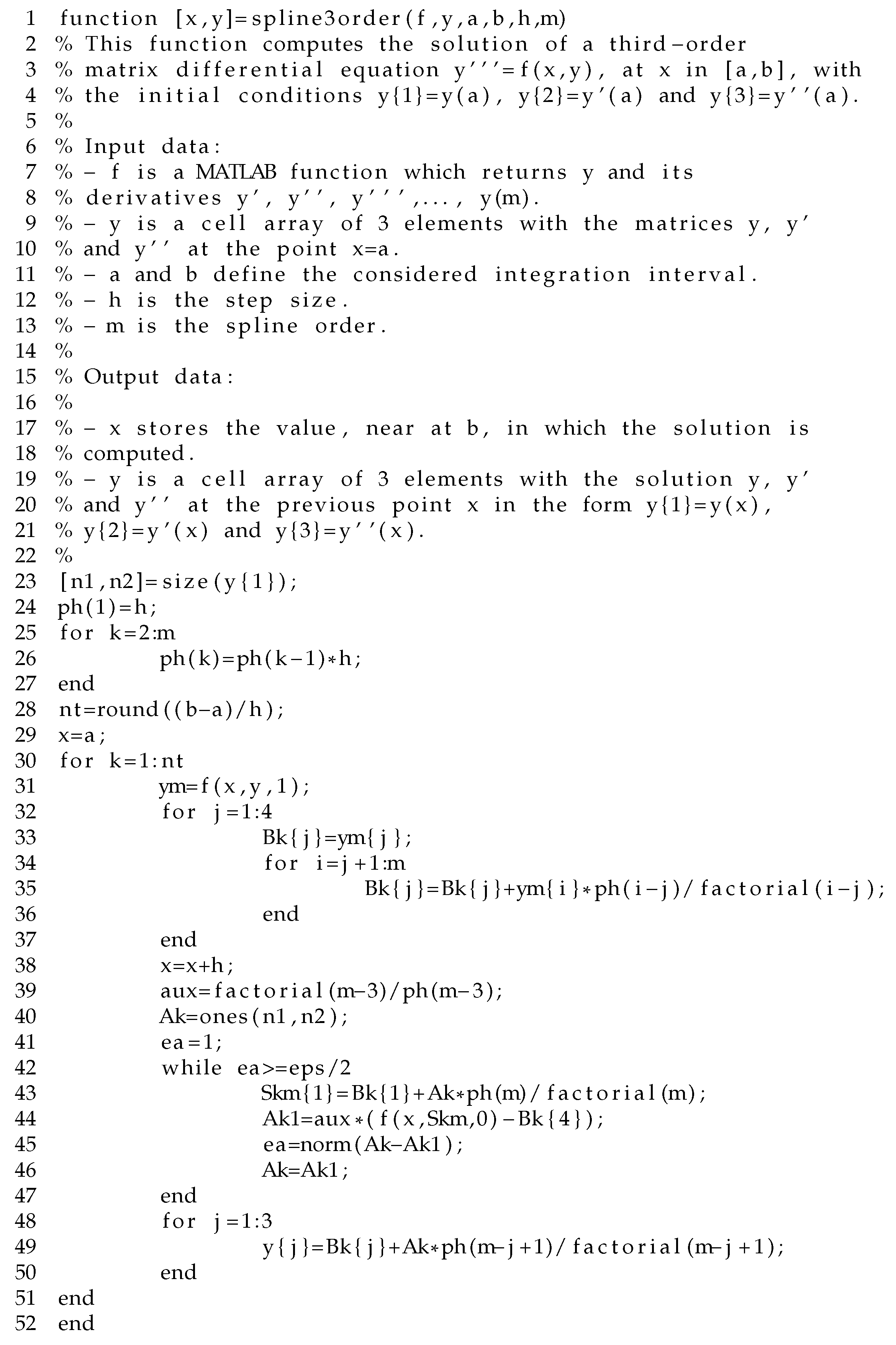
Figure 1 shows the MATLAB code that approximately computes the solution matrices
,
, and
of the third-order ordinary differential Equation (
4). This code uses the cell-array data type for storing sets of matrices. In Line 31,
, are obtained and stored in the cell-array variable
ym by invoking the
f MATLAB function to return the matrices that appear in expressions (
24)–(
27). In Lines 11–16, the expressions
,
,
, and
from Equations (
24)–(
27) are computed. In Lines 38–47, the matrix
is worked out by using the fixed-point iteration. Finally, in Lines 48–50,
,
, and
are computed approximately.
Figure 2 reproduces the MATLAB function
f for the thin-film flow of problem (
33). The dotted Line 24 indicates the completion of the list of all derivates until the
m-th one,
m being the spline order.
The memory requirements for this function are matrices, i.e., m matrices for the cell-array variable ym, 4 matrices for the cell-array variable Bk, 3 matrices for the variables Ak, Ak1, and Skm, and 3 matrices for the cell-array variable y.


