“Holographic Implementations” in the Complex Fluid Dynamics through a Fractal Paradigm

Abstract

Assimilating a complex fluid with a fractal object, non-differentiable behaviors in its dynamics are analyzed. Complex fluid dynamics in the form of hydrodynamic-type fractal regimes imply “holographic implementations” through velocity fields at non-differentiable scale resolution, via fractal solitons, fractal solitons–fractal kinks, and fractal minimal vortices. Complex fluid dynamics in the form of Schrödinger type fractal regimes imply “holographic implementations”, through the formalism of Airy functions of fractal type. Then, the in-phase coherence of the dynamics of the complex fluid structural units induces various operational procedures in the description of such dynamics: special cubics with SL(2R)-type group invariance, special differential geometry of Riemann type associated to such cubics, special apolar transport of cubics, special harmonic mapping principle, etc. In such a manner, a possible scenario toward chaos (a period-doubling scenario), without concluding in chaos (nonmanifest chaos), can be mimed.

1. Introduction

Common models used to describe the dynamics in complex fluids, are founded on a mix of basic theories, derived primarily from physics and computer simulations [1,2,3]. In such a context, their description implies both computational simulations based on specific algorithms [2], as well as developments on fundamental theories. With respect to models developed on fundamental theories, the following classes can be distinguished:

(i)

A class of models developed on spaces with integer dimension—i.e., differentiable models (for example, Navier–Stokes systems, etc.) [1,2,3];

(ii)

Another class of models developed on spaces with non-integer dimensions, which is clearly defined by means of fractional derivatives [4,5]—i.e., non-differentiable models, with examples including the fractal models [6];

(iii)

Expanding the previous class of models, new developments have been made based on Scale Relativity Theory. In such a context, the dynamics of any complex fluid can be developed on monofractal manifolds (theory of Nottale, in the fractal dimension D_f = 2) [7], or on the multifractal manifolds (as in the case of the Fractal Theory of Motion) [8,9].

Both in the context of Scale Relativity Theory in the sense of Nottale [7], as well as in the one of Fractal Theory of Motion [8,9], the fundamental hypothesis is the following: assuming that any type of complex fluid is assimilated to a fractal object, said dynamics can be analyzed using motions of the structural units of any complex fluid, on fractal curves.

Such a hypothesis may be illustrated by considering the following scenario: between two successive interactions of the structural units belonging to any complex system, the trajectory of the complex fluid’s structural unit is a straight line. This straight line becomes non-differentiable in the impact point. From such a perspective, taking into account that all interaction points construct an uncountable set of points, it can be stated that the trajectories of the complex fluid’s structural units become fractal curves. Given the diversity of the structural units which compose any complex fluid and the diversity of interactions taking place between them, extrapolating the preceding argument for any type of complex fluid, it results that it can be assimilated to a fractal in the general sense of Mandelbrot [6].

All these considerations imply that, in the description of complex fluid dynamics, instead of “working” with a single variable (regardless of its nature, i.e., velocity, density, etc.) governed through a non-differentiable function, it is necessary to “work” just with approximations of this function (i.e., mathematical function was given by averaging them on various scale resolutions). From such a perspective, it results that any mathematical variable purposed to characterize the complex fluid dynamics will act as the limit of a class of functions. Thus, said variable will be non-differentiable for null scale resolutions and differentiable otherwise [7,8,9]. To put it differently, from a mathematical point of view, these variables can be explained through fractal functions, i.e., functions dependent not only on spatial and temporal coordinates, but also on the scale resolution.

Because for a large temporal scale resolution when referring to the inverse of the highest Lyapunov exponent [10,11], the deterministic trajectories of any structural unit belonging to a complex fluid can be substituted by a “class” of virtual trajectories, such that the notion of a definite trajectory can be supplanted by the one of probability density. Considering all of the above, the fractality expressed by means of stochasticity, in the depiction of the dynamics of complex fluid, becomes operational in the fractal paradigm through the Fractal Theory of Motion [8,9].

In this context, the present study was directed to the modeling of the behavior of complex fluid dynamics. A mathematical model was created considering the complex fluid as a fractal object, and its dynamics were analyzed in the framework of Scale Relativity Theory [7,8,9].

2. Mathematical Model

The complex fluid is a collection of entities (or structured units) that, by means of their interactions, relationships, or dependencies construct a unified total. In what follows, the complex fluid will be assimilated with a fractal. Then, Scale Relativity Theory in the form of Fractal Theory of Motion becomes operational through the scale covariant derivative [8,9]:

$$\frac{\widehat{d}F}{dt}=\left[{\partial }_t+{\widehat{V}}^l{\partial }_l+\frac{1}{4}{\left(dt\right)}^{\left(\frac{2}{D_f}\right)-1}{D}^{lp}{\partial }_l{\partial }_p\right]F,$$

(1)

where

$$\begin{gathered} {\widehat{V}}^l=V_D^l-V_F^l \\ {D}^{lp}=d^{lp}-i{\widehat{d}}^{lp} \\ {d}^{lp}={\lambda }_{+}^l{\lambda }_{+}^p-{\lambda }_{-}^l{\lambda }_{-}^p \\ {\widehat{d}}^{lp}={\lambda }_{+}^l{\lambda }_{+}^p+{\lambda }_{-}^l{\lambda }_{-}^p \\ {\partial }_t=\frac{\partial }{\partial t}, {\partial }_l=\frac{\partial }{\partial x^l}, {\partial }_l{\partial }_p=\frac{\partial }{\partial x^l}\frac{\partial }{\partial x^p}, i=\sqrt{-1}, l,p=1,2,3 \end{gathered}$$

(2)

In relations (2), the meaning of the variables and parameters are as follows:

• $x^l$ is the fractal spatial coordinate;
• $t$ is the non-fractal time having the role of an affine parameter of the motion curves;
• ${\widehat{V}}^l$ is the complex velocity;
• $V_D^l$ is the differential velocity independent on the scale resolution;
• $V_F^l$ is the non-differentiable velocity dependent on the scale resolution;
• $dt$ is the scale resolution;
• $D_f$ is the fractal dimension of the movement curve;
• $D^{lp}$ is the constant tensor associated with the differentiable–non-differentiable transition;
• ${\lambda }_{+}^l\left({\lambda }_{+}^p\right)$ is the constant vector associated with the backward differentiable–non-differentiable dynamic processes;
• ${\lambda }_{-}^l\left({\lambda }_{-}^p\right)$ is the constant vector associated with the forward differentiable–non-differentiable dynamic processes;
• $F$ is a fractal function.

Many modes, and as such, an equally varied choice of definitions of fractal dimensions exist. More precisely, the fractal dimension of the Kolmogorov type and the fractal dimension of Hausdorff–Besikovitch type are the most frequently used [6,10,11]. Choosing one of the above fractal dimensions in the description of any complex fluid dynamics, the value of the fractal dimension must be constant and arbitrary in any dynamical analysis. For instance: $D_f<2$ for correlative processes in complex fluid dynamics, $D_f>2$ for non-correlative processes in said dynamics, etc. [10,11].

Accepting the functionality of the scale covariance principle, which refers to applying the operator (1) to the complex velocity field (2), for the case of free motions, the geodesics equation on fractal space takes the following form [8,9]:

$$\frac{\widehat{d}{\widehat{V}}^i}{dt}={\partial }_t{\widehat{V}}^i+{\widehat{V}}^l{\partial }_l{\widehat{V}}^i+\frac{1}{4}{\left(dt\right)}^{\left(\frac{2}{D_f}\right)-1}{D}^{lk}{\partial }_l{\partial }_k{\widehat{V}}^i=0,$$

(3)

This means that the fractal acceleration,${\partial }_t{\widehat{V}}^i$, the fractal convection, ${\widehat{V}}^l{\partial }_l{\widehat{V}}^i$ and the fractal dissipation, $D^{lk}{\partial }_l{\partial }_k{\widehat{V}}^i$, achieve their equilibrium at any point of the fractal curve.

If the fractalization is achieved by Markov-type stochastic processes (see Introduction and [6,7,8,9]), then:

$${\lambda }_{+}^i{\lambda }_{+}^l={\lambda }_{-}^i{\lambda }_{-}^l=2\lambda {\delta }^{il},$$

(4)

In (4), $\lambda$ is a coefficient linked to the differentiable-non-differentiable transition and ${\delta }^{il}$ is Kronecker’s pseudo-tensor. In these conditions, the geodesics Equation (3) becomes:

$$\frac{\widehat{d}{\widehat{V}}^i}{dt}={\partial }_t{\widehat{V}}^i+{\widehat{V}}^l{\partial }_l{\widehat{V}}^i-i\lambda {\left(dt\right)}^{\left(\frac{2}{D_f}\right)-1}{\partial }^l{\partial }_l{\widehat{V}}^i=0$$

(5)

3. Dynamics of Complex Fluids in the Form of Hydrodynamic—Type Fractal “Regimes”

The division of the complex fluid’s dynamics on scale resolutions implies, through (5), both the conservation law of the specific momentum at differentiable scale resolution:

$$\frac{\partial V_D^i}{dt}={\partial }_t{V}_D^i+V_D^l{\partial }_l{V}_D^i-\left[V_F^l+\lambda {\left(dt\right)}^{\left(\frac{2}{D_f}\right)-1}{\partial }_l\right]{\partial }^l{V}_F^i=0,$$

(6)

and also the conservation laws of the specific momentum at non-differentiable scale resolutions:

$$\frac{\partial V_F^i}{dt}={\partial }_t{V}_F^i+V_D^l{\partial }_l{V}_F^i+\left[V_F^l+\lambda {\left(dt\right)}^{\left(\frac{2}{D_f}\right)-1}{\partial }_l\right]{\partial }^l{V}_D^i=0,$$

(7)

From (6), it results that the specific force:

$$f_F^i=\left[V_F^l+\lambda {\left(dt\right)}^{\left(\frac{2}{D_f}\right)-1}{\partial }_l\right]{\partial }^l{V}_F^i,$$

(8)

induced by the velocity fields $V_F^i$. This becomes a “measure” of non-differentiability of motion curves of complex fluid entities.

In the case of stationary complex fluid dynamics $\left({\partial }_t{V}_D^i=0,{\partial }_t{V}_F^i=0\right)$, the conservation laws (6), (7) become:

$$V_D^l{\partial }_l{V}_D^i-\left[V_F^l+\lambda {\left(dt\right)}^{\left(\frac{2}{D_f}\right)-1}{\partial }_l\right]{\partial }^l{V}_F^i=0,$$

(9)

$$V_D^l{\partial }_l{V}_F^i+\left[V_F^l+\lambda {\left(dt\right)}^{\left(\frac{2}{D_f}\right)-1}{\partial }_l\right]{\partial }^l{V}_D^i=0,$$

(10)

while, in the static case (${\partial }_t{V}_D^i=0, V_D^i=0, {\partial }_t{V}_F^i=0$) these take the form:

$$\left[V_F^l+\lambda {\left(dt\right)}^{\left(\frac{2}{D_f}\right)-1}{\partial }_l\right]{\partial }^l{V}_F^i=0,$$

(11)

The result (11) specifies that, although at differentiable scale resolution, the complex fluid dynamics are absent while, at the non-differentiable scale resolution, the complex fluid dynamics can be “dictated” by the hydrodynamic fractal- type equations:

$$V_F^l{\partial }_l{V}_F^i+\lambda {\left(dt\right)}^{\left(\frac{2}{D_f}\right)-1}{\partial }_l{\partial }^l{V}_F^i=0$$

(12)

$${\partial }_l{V}_F^l=0$$

(13)

Equation (13) corresponds to the complex fluid incompressibility at the non-differentiable scale resolution (i.e., the states’ density ρ at the non-differentiable scale resolution is constant).

Generally, it is difficult to obtain an analytical solution for the previous equation system, taking into account its non-linear nature. However, it is still possible to obtain an analytic solution in the case of plane symmetry (for example, in ($x,$ $y$) coordinates) of the complex fluid dynamics. In order to obtain such a solution, in what follows, the method described in [12] will be used. Let it be considered the equations system (12) and (13) in the form:

$$U_0{\partial }_x{U}_0+V_0{\partial }_y{U}_0={\sigma }_0{\partial }_{yy}^2{U}_0,$$

(14)

$${\partial }_x{U}_0+{\partial }_y{V}_0=0,$$

(15)

where:

$$V_{Fx}=U_0\left(x,y\right), V_{Fy}=V_0\left(x,y\right), {\sigma }_0=\lambda {\left(dt\right)}^{\left(\frac{2}{D_f}\right)-1}$$

(16)

Imposing now the following conditions:

$$\underset{y\to 0}{\lim }{V}_0\left(x,y\right)=0, \underset{y\to 0}{\lim }\frac{\partial U_0}{\partial y}=0, \underset{y\to \infty }{\lim }{U}_0\left(x,y\right)=0,$$

(17)

and considering constant flux moment per unit of depth:

$$Q=\rho \underset{-\infty }{\overset{+\infty }{{\displaystyle \int }}}{U}_0^{2}dy=const.,$$

(18)

the velocity fields as the solution of the equations system (14) and (15), take the form:

$$U_0=\frac{1.5{\left(\frac{Q}{6\rho }\right)}^{\frac{2}{3}}}{{\left({\sigma }_{0}x\right)}^{\frac{1}{3}}}{\sec \mathrm{h}}^2\left[\frac{0.5y{\left(\frac{Q}{6\rho }\right)}^{\frac{1}{3}}}{{\left({\sigma }_{0}x\right)}^{\frac{2}{3}}}\right],$$

(19)

$$V_0=\frac{1.9{\left(\frac{Q}{6\rho }\right)}^{\frac{2}{3}}}{{\left({\sigma }_{0}x\right)}^{\frac{1}{3}}}\left\{\frac{y{\left(\frac{Q}{6\rho }\right)}^{\frac{1}{3}}}{{\left({\sigma }_{0}x\right)}^{\frac{2}{3}}}{\sec \mathrm{h}}^2\left[\frac{0.5y{\left(\frac{Q}{6\rho }\right)}^{\frac{1}{3}}}{{\left({\sigma }_{0}x\right)}^{\frac{2}{3}}}\right]-\tan \mathrm{h}\left[\frac{0.5y{\left(\frac{Q}{6\rho }\right)}^{\frac{1}{3}}}{{\left({\sigma }_{0}x\right)}^{\frac{2}{3}}}\right]\right\},$$

(20)

The previous can be simplified greatly through the use of non-dimensional variables:

$$X=\frac{x}{x_0}, Y=\frac{y}{y_0}, U=\frac{U_0}{w_0}, V=\frac{V_0}{w_0},$$

(21)

and non-dimensional parameters:

$$\mu =\frac{{\sigma }_0}{{\upsilon }_0}, {\upsilon }_0=\frac{y_0{}^{\frac{3}{2}}}{x_0}{\left(\frac{Q}{6\rho }\right)}^{\frac{1}{2}}, w_0=\frac{1}{{\left(y_0\right)}^{\frac{1}{2}}}{\left(\frac{Q}{6\rho }\right)}^{\frac{1}{2}},$$

(22)

where $x_0$, $y_0$, $w_0,$ and ${\nu }_0$ represent specific lengths, specific velocity, and “fractal degree” of the complex fluid dynamics. In these conditions, the normalized velocity fields become:

$$U=\frac{1.5}{{\left(\mu X\right)}^{\frac{1}{3}}}{\sec \mathrm{h}}^2\left[\frac{0.5Y}{{\left(\mu X\right)}^{\frac{2}{3}}}\right],$$

(23)

$$V=\frac{1.9}{{\left(\mu X\right)}^{\frac{1}{3}}}\left\{\frac{Y}{{\left(\mu X\right)}^{\frac{2}{3}}}{\sec \mathrm{h}}^2\left[\frac{0.5Y}{{\left(\mu X\right)}^{\frac{2}{3}}}\right]-\tan \mathrm{h}\left[\frac{0.5Y}{{\left(\mu X\right)}^{\frac{2}{3}}}\right]\right\},$$

(24)

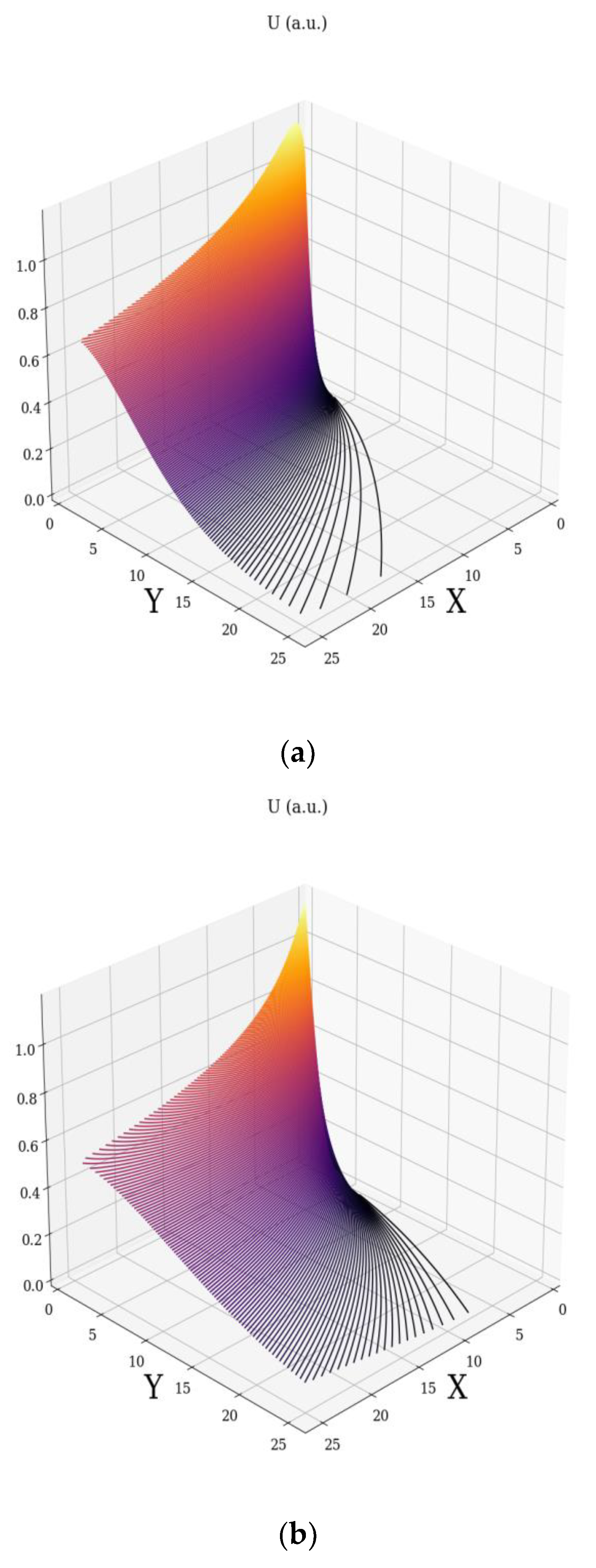
Any of the above relations describe the non-linear character of the velocity fields. This character can be explained through the fractal soliton (i.e., soliton depending on scale resolution) for the velocity field across the Ox axis, respectively “mixtures” of fractal soliton-fractal kink (i.e., kink dependent on scale resolution), for the velocity fields across the Oy axis. The specificities in the complex fluid dynamics are “explained” in Figure 1a–d and Figure 2a–d. Details on the soliton, kink, and other classical non-linear solutions are given in [10,11].

The velocity fields (23) and (24) induce the fractal minimal vortex (Figure 3a–d).

$$\begin{gathered} \mathsf{\Omega }=\left(\frac{\partial U}{\partial Y}-\frac{\partial V}{\partial Y}\right)=\frac{0.57Y}{{\left(\mu X\right)}^2}+\frac{0.63\mu }{{\left(\mu X\right)}^{\frac{4}{3}}}\tan \mathrm{h}\left[\frac{0.5Y}{{\left(\mu X\right)}^{\frac{2}{3}}}\right]+\frac{1.9Y}{{\left(\mu X\right)}^2}{\sec \mathrm{h}}^2\left[\frac{0.5Y}{{\left(\mu X\right)}^{\frac{2}{3}}}\right]- \\ -\frac{0.57Y}{{\left(\mu X\right)}^2}{\tan \mathrm{h}}^2\left[\frac{0.5Y}{{\left(\mu X\right)}^{\frac{2}{3}}}\right]-\left[\frac{1.5}{\mu X}+\frac{1.4Y^2}{X{\left(\mu X\right)}^{\frac{5}{3}}}\right]{\sec \mathrm{h}}^2\left[\frac{0.5Y}{{\left(\mu X\right)}^{\frac{2}{3}}}\right]\tan \mathrm{h}\left[\frac{0.5Y}{{\left(\mu X\right)}^{\frac{2}{3}}}\right], \end{gathered}$$

(25)

This previous result was used to specify the fact that the turbulence sources may be induced by fractal vortices. As long as the complex fluid is not constrained externally, fractal vortices do not manifest themselves. Phrasing it differently, they are “virtual” fractal vortices and manifest as “virtual” turbulence sources. In the presence of an external constraint, they become “real” and the turbulence mechanism is triggered. Essentially, the discussion revolves around “holographic implementation” of turbulences in the complex fluid dynamics. It is reminded that, since the dynamics of complex fluid entities are described by continuous but non-differentiable curves, curves which exhibit the property of self-similarity in every one of its points, these can be viewed as a holographic mechanism (every part reflects the whole) of dynamics description. It is noted that the previous choice of the fractality degree (i.e., the scale resolution, type of motion curve through its fractal dimension) can generally cover various types of dynamics found in complex fluids. Moreover, it is noted that the previous Figures were obtained in a Python programming environment.

4. Dynamics of Complex Fluids in the Form of Schrödinger-Type “Regimes”

In the case of irrotational motions of the complex fluid structural units, the complex velocity field ${\widehat{V}}^i$ from (2) becomes:

$${\widehat{V}}^i=-2i\lambda {\left(dt\right)}^{\left(\frac{2}{D_f}\right)-1}{\partial }^i\ln \mathsf{\Psi }$$

(26)

where $\ln \mathsf{\Psi }$ is the fractal scalar potential of the velocity fields and $\mathsf{\Psi }$ is a fractal state function.

Then, substituting (26) in (5), the geodesics Equation (5) becomes (for details on the method, see [7,8,9]):

$${\lambda }^2{\left(dt\right)}^{\left(\frac{4}{D_f}\right)-2}{\partial }^l{\partial }_l\mathsf{\Psi }+i\lambda {\left(dt\right)}^{\left(\frac{2}{D_f}\right)-1}{\partial }_t\mathsf{\Psi }=0$$

(27)

Relation (27) is a Schrödinger equation of fractal type. As a consequence, different dynamics of any complex fluids can be explained as Schrödinger-type fractal “regimes”. In the particular case of the dynamics of structural units belonging to the complex fluid, on Peano-type curves ($D_f\to 2$) at Compton scale ($\lambda =h/4\pi m_0$, where $h$ is Planck’s constant and $m_0$ is the rest mass of the structural unit belonging to the complex fluid), (27) becomes the standard Schrödinger equation from quantum mechanics.

The solution of the one-dimensional Schrödinger equation of fractal type can be written in the form (for details see [13,14]):

$$\begin{gathered} \mathsf{\Psi }\left(x,t\right)=\frac{1}{\sqrt{t}}exp\left(i\frac{x^2}{4\mu t}\right), \\ \mu =\lambda {\left(dt\right)}^{\left(\frac{2}{D_f}\right)-1} \end{gathered}$$

(28)

and is defined, of course, up to an arbitrary multiplicative constant.

As such, the general solution of Equation (27) can be written as a linear superposition of the form:

$$\mathsf{\Psi }\left(x,t\right)=\frac{1}{\sqrt{t}}\underset{-\infty }{\overset{+\infty }{{\displaystyle \int }}}u\left(y\right)exp\left[i\frac{{\left(x-y\right)}^2}{4\mu t}\right]dy$$

(29)

Now, if $u\left(y\right)$ is an Airy function of fractal type, then $\mathsf{\Psi }\left(x,t\right)$ retains this property, in the sense that its amplitude is an Airy function of fractal type. Indeed, in this case, there will be:

$$u\left(y\right)\equiv Ai\left(y\right)=\frac{1}{2\pi }\underset{-\infty }{\overset{+\infty }{{\displaystyle \int }}}exp\left[i\left(\frac{{\omega }^3}{3}+\omega y\right)\right]d\omega$$

(30)

in such a way as the state function (29) will be written in the form:

$$\mathsf{\Psi }\left(x,t\right)=\frac{1}{2\pi \sqrt{t}}\underset{-\infty }{\overset{+\infty }{{\displaystyle \int }}}exp\left\{i\left[\frac{{\omega }^3}{3}+\omega y+\frac{{\left(x-y\right)}^2}{4ut}\right]\right\}dyd\omega$$

(31)

If, at first, the integration will be carried out after $y$, up to a multiplicative constant, the results is:

$$\mathsf{\Psi }\left(x,t\right)=\frac{1}{2\pi }\underset{-\infty }{\overset{+\infty }{{\displaystyle \int }}}exp\left[i\left(\frac{{\omega }^3}{3}+\omega x-\mu t{\omega }^2\right)\right]d\omega$$

(32)

The final result is obtained based on a special relationship developed in [13,14] and it is:

$$\mathsf{\Psi }\left(x,t\right)=\left[Ai\left(kx-{\nu }^2{t}^2\right)\right]exp\left[i\nu t\left(kx-\frac{2}{3}{\nu }^2{t}^2\right)\right]$$

(33)

with

$$\nu =k^2\mu$$

(34)

In these conditions, if $\mathsf{\Psi }$ is chosen in the form:

$$\mathsf{\Psi }\left(x,t\right)=A\left(x,t\right)\exp \left[i\varphi \left(x,t\right)\right]$$

(35)

where $A\left(x,t\right)$ is an amplitude and $\mathsf{\Phi }\left(x,t\right)$ is a phase, by identifying in (33) the amplitude and the phase, there will be:

$$\begin{gathered} A\left(x,t\right)=Ai\left(kx-{\nu }^2{t}^2\right), \\ \varphi \left(x,t\right)=\nu t\left(kx-\frac{2}{3}{\nu }^2{t}^2\right) \end{gathered}$$

(36)

By substituting (35) in (27), by means of direct calculation, the following relation is checked:

$$i\partial \mathsf{\Psi }+\mu {\partial }_l{\partial }^l\mathsf{\Psi }=-\left[{\partial }_t\varphi +\mu {({\partial }_l\varphi )}^2-\mu \frac{{\partial }_l{\partial }^l\mathrm{A}}{A}\right]+\frac{i}{2A^2}\left[{\partial }_t{A}^2+2\mu {\partial }_l\left(A^2{\partial }^l\varphi \right)\right]$$

(37)

Now, the “specific constraints” necessary for $\mathsf{\Psi }$ to be a solution of the non-stationary differential Equation (37) will be reducible to the differential equations:

$$\begin{gathered} {\partial }_t\varphi +\mu \left({\partial }_l\varphi {\partial }^l\varphi \right)=\mu \frac{{\partial }_l{\partial }^{l}A}{A} \\ {\partial }_t{A}^2+2\mu \left(A^2{\partial }_l\varphi \right)=0 \end{gathered}$$

(38)

The first of these equations is the Hamilton–Jacobi equation of fractal type, while the second equation is the continuity equation of fractal type. From here, the correspondence with the hydrodynamic model of fractal type, pertaining to scale relativity [7,8,9], becomes evident based on the substitutions:

$$\begin{gathered} V_D^i=\mu {\partial }^i\varphi , \\ \rho =A^2 \end{gathered}$$

(39)

where $V_D^i$ is the differential component of the velocity field and $\rho$ is the density of states. In this condition, the conservation law of fractal type of the specific momentum:

$${\partial }_t{V}_D^i+V_D^l{\partial }_l{V}_D^i=-{\partial }^{i}Q$$

(40)

and respectively, the conservation law of the density of states of fractal type:

$${\partial }_t\rho +{\partial }^l\left(\rho V_D^l\right)=0$$

(41)

can be found.

The specific potential of fractal type:

$$Q=-{\mu }^2\frac{{\partial }_l{\partial }^l\sqrt{\rho }}{\sqrt{\rho }}$$

(42)

through the induced specific force of fractal type:

$$f^i=-{\partial }^{i}Q=-{\mu }^2{\partial }^i\left(\frac{{\partial }_l{\partial }^l\sqrt{\rho }}{\sqrt{\rho }}\right)$$

(43)

becomes a measure of the fractal degree pertaining to the motion curves.

Now, through (36), the in-phase coherence of the structural unit dynamics for any complex fluid implies the condition

$$\mathsf{\Phi }\left(x, t\right)=\nu t\left(kx-\frac{2}{3}{\nu }^2{t}^2\right)=const$$

(44)

or, moreover, in the notations:

$$-\frac{2}{3}{\nu }^3{t}^3=a_0{X}^3, a_1=0, \nu kxt=3a_2, a_3=const.$$

the cubic equation:

$$a_0{X}^3+3a_1{X}^2+3a_{2}X+a_3=0$$

(45)

If (45) has real roots [14,15]:

$$\begin{gathered} X_1=\frac{h+\overline{h}k}{1+k}, \\ {X}_2=\frac{h+\epsilon \overline{h}k}{1+\epsilon k}, \\ {X}_3=\frac{h+{\epsilon }^2\overline{h}k}{1+{\epsilon }^{2}k} \end{gathered}$$

(46)

with $h$, $\overline{h}$ the roots of Hessian, and $\epsilon \equiv \left(-1+i\sqrt{3}\right)/2$ the cubic root of unity $\left(i=\sqrt{-1}\right)$, the values of variables $h$, $\overline{h,}$ and $k$ can be “scanned” by a simple transitive group with real parameters. This group can be revealed through Riemann-type spaces associated with the previous cubic. The basis of this approach is the fact that the simply transitive group with real parameters [14,15]:

$$X_l\leftrightarrow \frac{a{X}_l+b}{c{X}_l+d} , l=1,2,3 a,b,c,d\in R$$

(47)

where $X_l$ are the roots of the cubic (45), induces the simply transitive group in the quantities $h$, $\overline{h},$ and $k$, whose actions are:

$$\begin{gathered} h\leftrightarrow \frac{ah+b}{ch+d}, \\ \overline{h} \leftrightarrow \frac{a\overline{h}+b}{c\overline{h}+d}, \\ k\leftrightarrow \frac{c\overline{h}+d}{ch+d}k \end{gathered}$$

(48)

The structure of this group is typical of SL(2R), i.e.,

$$\begin{gathered} \left[B^1,B^2\right]=B^1, \\ \left[B^2,B^3\right]=B^3, \\ \left[B^3,B^1\right]=-2B^2 \end{gathered}$$

(49)

where $B^l$ are the infinitezimal generators of the group:

$$\begin{gathered} B^1=\frac{\partial }{\partial h}+\frac{\partial }{\partial \overline{h}} \\ {B}^2=h\frac{\partial }{\partial h}+\overline{h}\frac{\partial }{\partial \overline{h}} \\ {B}^3=h^2\frac{\partial }{\partial h}+{\overline{h}}^2\frac{\partial }{\partial \overline{h}}+\left(h-\overline{h}\right)k\frac{\partial }{\partial k} \end{gathered}$$

(50)

and admit the absolute invariant differentials

$$\begin{gathered} {\omega }^1=\frac{dh}{\left(h-\overline{h}\right)k} \\ {\omega }^2=-i\left(\frac{dk}{k}-\frac{dh+d\overline{h}}{h-\overline{h}}\right) \\ {\omega }^3=-\frac{kd\overline{h}}{h-\overline{h}} \end{gathered}$$

(51)

and the 2-form (the metric):

$$d{s}^2={\left(\frac{dk}{k}-\frac{dh+d\overline{h}}{h-\overline{h}}\right)}^2-4\frac{dhd\overline{h}}{{\left(h-\overline{h}\right)}^2}$$

(52)

In real terms

$$h=u+iv, \overline{h}=u+iv, k=e^{i\theta }$$

(53)

and for

$$\begin{gathered} {\mathsf{\Omega }}^1={\omega }^2=d\theta +\frac{du}{v} \\ {\mathsf{\Omega }}^2=\cos \theta \frac{du}{v}+\sin \theta \frac{dv}{v} \\ {\mathsf{\Omega }}^3=-\sin \theta \frac{du}{v}+\cos \theta \frac{dv}{v}, \end{gathered}$$

(54)

the connection with Poincaré representation of the Lobachevsky plane can be obtained. Indeed, the metric is a three-dimensional Lorentz structure:

$$d{s}^2=-{\left({\mathsf{\Omega }}^1\right)}^2+{\left({\mathsf{\Omega }}^2\right)}^2+{\left({\mathsf{\Omega }}^3\right)}^2=-{\left(d\theta +\frac{du}{v}\right)}^2+\frac{d{u}^2+d{v}^2}{v^2}$$

(55)

This metric reduces to that of Poincaré, in cases where ${\mathsf{\Omega }}^1\equiv 0,$ which defines the variable $\theta$ as the “angle of parallelism” of the hyperbolic planes (the connection). In fact, recalling that

$$\frac{dk}{k}-\frac{dh+d\overline{h}}{h-\overline{h}}=0\leftrightarrow d\theta =-\frac{du}{v}$$

(56)

represents the connection form of the hyperbolic plane, the relationship (54) then represents general Bäcklund transformations in that plane. In such a conjecture, it is noted that, if the temporal cubic is assumed to have distinct roots, the condition (56) is satisfied, if, and only if, the differential forms ${\mathsf{\Omega }}^1$ is null.

Therefore, for the metric (55) with restriction (56), the relation becomes:

$$d{s}^2=\frac{dhd\overline{h}}{{\left(h-\overline{h}\right)}^2}=\frac{d{u}^2+d{v}^2}{v^2}$$

(57)

The parallel transport of the hyperbolic plane actually represents the apolar transport of the cubics (45).

Such a metric approach allows harmonic mappings from the usual space to the hyperbolic one (space associated to the dynamics of the complex fluid), through the functional (for details see [14,15,16]):

$$J=\frac{1}{2}\iiint d^3\mathit{X}\left[\frac{{\partial }_{l}h{\partial }^l\overline{h}}{{\left(h-\overline{h}\right)}^2}\right]$$

(58)

where the usual notation ${\partial }_l$ denotes the gradient and $d^3\mathit{X}$ is the elementary volume.

In the case of the synchronization of dynamics of any complex fluid structural units, i.e., in-phase coherence through the condition (44), the Euler equations corresponding to the functional (58) is:

$$\left(h-\overline{h}\right)\nabla \left(\nabla h\right)=2{\left(\nabla h\right)}^2$$

(59)

which admits

$$h=i\frac{\cosh \chi -\sinh \chi e^{-i\overline{\mathsf{\Omega }}}}{\cosh \chi +\sinh \chi e^{-i\overline{\mathsf{\Omega }}}}, \chi =\frac{\psi }{2}$$

(60)

as a solution, as long as $\chi$ (and thus $\psi$) are solutions of a Laplace-type equation for the free space.

Therefore, space-time “synchronization modes” in phase and amplitude of the complex fluid structural units imply group invariances of a $SL\left(2R\right)$ type. Then, period doubling emerges as a natural behavior in the complex fluid dynamics (see Figure 4a–c where $r=tanh\chi$, $\left|h\right|\equiv Amplitude$ and $\overline{\mathsf{\Omega }}=\mathsf{\Omega }\mathrm{t}$ at various scale resolutions, given by means of the maximum value of $\mathsf{\Omega }$, i.e.,${ \mathsf{\Omega }}_{max}$).

As it can be observed in Figure 4a–c, the natural transition of a complex fluid is to evolve from a normal period doubling state towards damped oscillating and strong modulated dynamics. The complex fluid never reaches a chaotic state, but it permanently evolves towards that state. There is a periodicity to the whole series of transitions, the system evolves through period doubling, damped oscillations even reaching in some cases an intermittent state (the damped oscillations, intermittent states, etc. will be analyzed by us in a future paper), but it never reaches a pure chaotic state. The evolution of the systems sees a “jump” into a period doubling oscillation state and the transition resumes towards a quasi-chaotic state.

The Bifurcation Map is presented (Figure 5) where again it is observed that the complex fluid starts from a steady state (double period state) and evolves towards a chaotic one (${\mathsf{\Omega }}_{max}=2$) but it never reaches that state. For each periodic transition scenario, it is possible to observe the system swiping through all the previously mentioned dynamic states. Therefore, there is an overall periodicity with a continuous increase in oscillation amplitude.

Let it be noted that the mathematical formalism of the Fractal Theory of Motion implies various operational procedures (invariance groups, harmonic mappings, groups isomorphism, embedding manifolds, etc.) with quite a number of applications in complex fluid dynamics [17,18].

5. Conclusions

Assimilating the complex fluid with a fractal, different dynamics at various scale resolutions are analyzed. Therefore, the following conclusions may be stated:

(i)

The complex fluid dynamics, in the form of hydrodynamic-type fractal regimes, specify velocity fields at non-differentiable scale resolution, in the form of fractal solitons, fractal solitons–fractal kinks, and fractal minimal vortices;

(ii)

The fractal vortices can be linked to turbulence sources in complex fluid dynamics at non-differentiable scale resolutions. So long as they are not acted upon by any external constraint, fractal vortices are virtual and non-manifest. However, the presence of external constraints radically changes the complex fluid dynamics, in the sense that the vortices will manifest as a real turbulences. Since the dynamics of complex fluid entities are described by continuous but non-differentiable curves (which exhibit the property of self-similarity in every one of their points), these can be viewed as a holographic mechanism (every part reflects the whole) in the description of complex fluid dynamics;

(iii)

The description of the complex fluid dynamics in the form of Schrödinger type-fractal regimes imply “holographic implementations”, through the formalism of Airy functions of fractal type. From such a perspective, the in-phase coherence of the dynamics of the complex fluid structural units induces various operational procedures in the description of such dynamics: special cubics with SL(2R)-type group invariance, special differential geometry of Riemann type associated to such cubics, special apolar transport of cubics, special harmonic mapping principle, etc. Referring to the special harmonic principle, in-phase coherence allows harmonic mappings from the usual space to the hyperbolic one, situation in which the period doubling “synchronization mode” among the structural units of a complex fluid becomes functional. In such a manner, a possible scenario toward chaos (period doubling scenario), without concluding in chaos (nonmanifest chaos), can be mimed.