Quasi-Deterministic Processes with Monotonic Trajectories and Unsupervised Machine Learning

Abstract

This paper aims to consider approximation-estimation tests for decision-making by machine-learning methods, and integral-estimation tests are defined, which is a generalization for the continuous case. Approximation-estimation tests are measurable sampling functions (statistics) that estimate the approximation error of monotonically increasing number sequences in different classes of functions. These tests make it possible to determine the Markov moments of a qualitative change in the increase in such sequences, from linear to nonlinear type. If these sequences are trajectories of discrete quasi-deterministic random processes, then moments of change in the nature of their growth and qualitative change in the process match up. For example, in cluster analysis, approximation-estimation tests are a formal generalization of the “elbow method” heuristic. In solid mechanics, they can be used to determine the proportionality limit for the stress strain curve (boundaries of application of Hooke’s law). In molecular biology methods, approximation-estimation tests make it possible to determine the beginning of the exponential phase and the transition to the plateau phase for the curves of fluorescence accumulation of the real-time polymerase chain reaction, etc.

1. Introduction

Many questions originating from the classical works of P. L. Chebyshev and A. A. Markov on approximation methods are of significant theoretical and great practical importance. The generalized Markov moment problem is closely related to problems of geometry, algebra, and function theory. From this point of view, it is possible to study not only tasks of the Petersburg mathematical school “on the limiting values of integrals”, but also problems of the theory of approximation, interpolation and extrapolation in various classes of functions [1].

It is also interesting that not only the main theorems and statements and the accompanying auxiliary and preparatory results help solve applied problems. It turned out to be possible to use some of them to solve modern artificial intelligence problems, such as machine-learning methods. Today, several types of machine learning are known: supervised, semi-supervised, unsupervised, and reinforcement learning. Unsupervised learning is a type of machine learning that makes decisions or searches for patterns in a set of unlabeled data. He is designed to solve three types of problems: clustering, dimensionality reduction, and anomaly detection.

Cluster analysis is a multivariate statistical procedure for training a set of labels on a sample of unlabeled data. The range of applications of cluster analysis is extensive: it is used in archeology, medicine, psychology, chemistry, biology, public administration, philology, anthropology, marketing, sociology, geology, and other disciplines. However, the universality of application has led to the emergence of many conflicting terms, methods, and approaches. This universality complicates the unambiguous use and consistent interpretation of cluster analysis. There are many clustering algorithms, and it is difficult to say which one will be the most adequate for a given dataset.

Hierarchical methods form a tree-like structure of cluster formation, which is commonly called a dendrogram. New clusters are formed from the previously formed clusters [2,3]. Another approach to solving the clustering problem in Euclidean space is based on the estimation of the distribution density of the elements of the sample population, for example, the methods DBSCAN [4] and OPTICS [5,6]. Splitting methods break objects into a priori a given number of clusters. They are used to optimize the similarity function of objective criteria, for example, when distance is the main parameter. The most famous of these algorithms is the K-means method [2,3]. Grid-based methods form the data space as a finite number of cells that form a grid-like structure. All clustering operations performed on these grids are independent of the number of data [7].

In statistics, machine learning, and information theory, dimensionality reduction is the transformation of data, which reduces the number of variables by deriving the principal variables. Dimensionality reduction of the data removes redundant or highly correlated features and reduces the amount of noise in the data. This transformation of data allows simpler mathematical models that are easier and more transparent to interpret. In practice, the following methods are commonly used for dimensionality reduction: Principal Component Analysis, Uniform Manifold Approximation and Projection, Discriminant Analysis, and Autoencoders [8,9].

The task of anomaly detection is to identify data significantly different from the typical elements of some set. Anomalies are also referred to as outliers, novelties, noise, deviations, and exceptions [10,11]. In particular, in the context of network intrusion detection, objects of interest are often not rare objects but unexpected bursts of activity. This pattern does not follow the general statistical definition of an outlier as a rare object, and many outlier detection methods (in particular, uncontrolled methods) do not work with such data [12].

Sometimes we can consider anomaly detection by unsupervised machine-learning methods as a sequential statistical analysis of monotone trajectories $y_t$ of a discrete quasi-deterministic process $\xi$. For example, solving cluster analysis problems, solid mechanics problems, molecular biology, switched systems, etc.

The main idea of the approach proposed in this article has a pioneering character and is as follows. If a quasi-deterministic process $\xi$ with monotone trajectories $y_t$ is studied, then the moment $t_0$ of the change in the character of their increase from linear to nonlinear type may coincide with a qualitative change $\xi$. Analytically, this moment can be determined by comparing the squared error of the linear approximation of the trajectory $y_t$ with the squared errors of the nonlinear approximation of the same trajectory. The difference in such errors is a quadratic form. This quadratic form changes the sign at the point $t_0$ if the point is of qualitative change of the trajectory $y_t$. The coefficients of the approximating functions are sought using the least-squares method by of the $y_{t_0-k},\dots ,y_{t_0-2},y_{t_0-1}$, from the left semi-neighborhood of the point $t_0$.

It is noteworthy that in our study, we use a whole set of mathematical concepts bearing the name of the outstanding Russian scientist A. A. Markov. In addition to the constructions accompanying the generalized problem of Markov moments, this is a Markov decision process, a Markov moment in time in the theory of random processes, and a Markov chain with memory.

2. Quasi-Deterministic Processes, Markov Moments and Markov Decision Process

Let $T=\overline{1,m-1}$ be a finite subset of the sequence of natural numbers. The family $\xi =\{{\xi }_t,t\in T\}$ of random variables ${\xi }_t={\xi }_t\left(\omega \right)$, given on the probability space $(\Omega ,\mathcal{F},\mathrm{P})$ is called a discrete random process [13,14]. Each random variable ${\xi }_t$ generates an $\sigma$-algebra, which we will denote by as ${\mathcal{F}}_{{\xi }_t}$ [15]. The $\sigma$-algebra generated by the random process $\xi =\{{\xi }_t,t\in T\}$ is the minimal $\sigma$-algebra containing all, ${\mathcal{F}}_{{\xi }_t}$ i.e.,

$$\sigma \left(\xi \right)=\sigma \left(\bigcup _{t=1}^{m-1}{\mathcal{F}}_{{\xi }_t}\right).$$

(1)

If we fix a time, t then obtain a random variable ${\xi }_t$. If we fix a random event ${\omega }_0$, then obtain a trajectory of the random process $\xi$, which is a random sequence $y_t={\xi }_t\left({\omega }_0\right)$.

Random processes can be divided into two classes: quasi-deterministic processes and non-deterministic processes. We will consider only quasi-deterministic processes with monotonic trajectories. A random process $\xi =\xi (t,\omega )$ is called quasi-deterministic if all sequences $y_t$ are functions of time of a given form, but each of them depends on a random parameter $\omega$. In general, $\omega$ can be a randomly selected number, a random vector, a random sequence, or a random function. The main property of any quasi-deterministic process is that each random event $\omega$ corresponds to only one trajectory $y_t$ of the random process $\xi =\xi (t,\omega )$ [16].

2.1. Markov Stopping Time

We will consider the binary problem of testing the statistical hypotheses $H_0$ and $H_1$. The null hypothesis $H_0$—the sequence $y_t$ increases linearly, and the alternative hypothesis $H_1$—the sequence $y_t$ increases nonlinearly.

To test a statistical hypothesis, it will be necessary to construct a criterion allowing it to be accepted or rejected. Statistical criteria are based on a random set X. Two variants are possible; in the first, the sample X is extracted from the n -dimensional Euclidean space ${\mathbb{E}}^n$ at once, i.e., it has a fixed volume. The second, when the sample X is generated over a period of time, and its size is a random variable [17]. A combined case is possible when X is extracted from ${\mathbb{E}}^n$ at once, and then its variable size subsample is studied, which is formed by mapping X into itself. In the last two cases, one speaks of sequential statistical analysis and sequential statistical test [18,19].

Decision-making at a certain moment of time can be based only on the known values of the discrete process $\xi =\xi (t,\omega )$. If we use a formal approach, then the events under study should be measurable in a non-decreasing sequence of $\sigma$ -algebras ${\mathfrak{F}}_k$ generated by the process $\xi =\xi (t,\omega )$ [20]. On the probability space, $(\Omega ,\mathcal{F},\mathrm{P})$ such a sequence is considered to be a family of $\sigma$-algebras $\mathfrak{F}=\{{\mathcal{F}}_t,t\in T\}$ and is called a filtration if for $\forall i,j\in T|i<j:{\mathcal{F}}_i\subset {\mathcal{F}}_j\subset \mathcal{F}$. The map $\tau :\Omega ⟶T$ is called the Markov moment with respect to the filtration $\mathfrak{F}$, if for $\forall t\in T$ is the preimage of the set $\{\tau \le t\}\in {\mathcal{F}}_t$. If moreover $Pr(\tau <+\infty )=1$, then $\tau$ is called the Markov stopping time [21].

For example, a random event $\omega$ belongs to $\Omega$ from the previously introduced probability space $(\Omega ,\mathcal{F},\mathrm{P})$. If this random event $\omega$ is the extraction of a finite set X from the n-dimensional Euclidean space, ${\mathbb{E}}^n$ then any point $\overline{x}\in {\mathbb{E}}^n$ can belong to the set X. By definition, the $\sigma$-algebra from the $(\Omega ,\mathcal{F},\mathrm{P})$ contains all ${\mathbb{E}}^n$. In addition, this $\sigma$-algebra contains any finite set X from the space ${\mathbb{E}}^n$, all possible countable unions of such sets and complements to hims. We denote this system of sets as $\mathcal{S}\left({\mathbb{E}}^n\right)$. The same reasoning is valid for any $\sigma$-algebra ${\mathcal{F}}_{{\xi }_t}$, therefore $\sigma \left(\xi \right)=\mathcal{S}\left({\mathbb{E}}^n\right).$ These $\sigma$-algebra $\mathcal{S}\left({\mathbb{E}}^n\right)$ will be filtration for $\xi =\xi (t,\omega )$ [22,23].

If a random event $\omega \in \Omega$ is the extraction of a countable set X from the n-dimensional Euclidean space ${\mathbb{E}}^n$, then the filtration for $\xi =\xi (t,\omega )$ will again be the $\sigma$-algebra $\mathcal{S}\left({\mathbb{E}}^n\right)$. If the event $\omega \in \Omega$ is some random function $f\left(x\right)$, then the filtration for $\xi =\xi (t,\omega )$ is Borel’s $\sigma$-algebra $\mathcal{B}\left({\mathbb{E}}^n\right)$.

In all these cases, the Markov stopping time is the minimum value $\tau$ at which the null hypothesis is rejected—$H_0$ (the trajectory of the quasi-determinate process $\xi =\xi (t,\omega )$ increases linearly) and an alternative hypothesis is accepted—$H_1$ (the trajectory of the quasi-determinate process $\xi =\xi (t,\omega )$ increases nonlinearly).

2.2. Approximation-Estimation Tests

To test the statistical hypotheses $H_0$ and $H_1$, we use the approximation-estimation tests [24,25]. We will construct quadratic forms of approximation-estimation tests as the difference between the quadratic error of the linear approximation of the numerical sequence $y_t$ and the quadratic error of the nonlinear approximation of $y_t$ in various classes of nonlinear functions.

Let us use the concept of an approximating function. Ordered pairs $(i,y_i)$ are the knots of approximation for the numerical sequence $y_t$ where i is a natural argument, $y_i$ is the corresponding value of the sequence $y_t$. We will be called $(i,y_i)$ the natural knot of approximation [24,25].

The segment of the real axis $[y_0,y_{k-1}]$, on which the knots $y_0,y_1,\dots ,y_{k-1}$ are located, will be called the “current interval of approximation”.

Let a real function $f\left(t\right)$ belong to class Y. The function $f\left(t\right)$ approximates a numerical sequence $y_t$ by the least-squares method if

$${\delta }^2=\underset{f\in Y}{mín}\sum _{i=0}^{k-1}{(f\left(i\right)-y_i)}^2.$$

(2)

There is always such the minimum since ${\delta }^2$ is a positive definite quadratic form.

The quadratic error of approximation of the numerical sequence $y_t$ by an arbitrary nonlinear function $f\left(t\right)$ is equal to the sum of the squares of the differences $y_t$ and $f\left(t\right)$ at the knots $y_0,y_1,\dots ,y_{k-1}$ for the corresponding values of the natural argument.

$${\delta }_f^2\left(k_0\right)=\sum _{i=0}^{k-1}{(f\left(i\right)-y_i)}^2.$$

(3)

The quadratic error of $y_t$ linear approximation with respect to the same knots is equal to:

$${\delta }_l^2\left(k_0\right)=\sum _{i=0}^{k-1}{(a·i+b-y_i)}^2.$$

(4)

If in our reasoning, the specific number of approximation knots does not play a role, then the quadratic errors will be denoted by ${\delta }_f^2$ and ${\delta }_l^2$. These errors calculate from Formulas (3) and (4) respectively.

Let us introduce the notation: $m=mín({\delta }_l^2,{\delta }_f^2)$.

We assume by definition that the increase in the numerical sequence $y_t$ along the knots $y_0,y_1,\dots ,y_{k-1}$ is linear if $m={\delta }_l^2$. Otherwise, the increase in $y_t$ has a nonlinear character. If ${\delta }_l^2={\delta }_f^2$, then the point $y_{k-1}$ is called “critical”.

When constructing quadratic forms of approximation-estimation tests, can use a technique that facilitates calculations. The values of $y_t$ can be taken at the points, $y_0,y_1,\dots ,y_{k-1}$ assuming that $y_0=0$. This condition can be easily achieved at any approximation step using the transformation:

$$y_0=y_j-y_j,y_1=y_{j+1}-y_j,\dots ,y_{k-1}=y_{j+k-1}-y_j.$$

(5)

It is possible to construct several approximation-estimation tests, for example, logarithmic, parabolic, exponential, etc. In the general case, the approximation-estimation test can be formulated as follows.

Let ${\delta }^2\left(k_0\right)={\delta }_l^2\left(k_0\right)-{\delta }_f^2\left(k_0\right)$. We will say that at the left semi-neighborhood of the point k (between points $k-1$ and k) is the character of the increase of the sequence $y_t$ has changed from linear to nonlinear, if the following conditions hold: for the knots $y_0,y_1,\dots ,y_{k-1}$ is true ${\delta }^2\left(k_0\right)\le 0$, and for the knots $y_1,y_2,\dots ,y_k$ is true ${\delta }^2\left(k_0\right)>0$. If we use terms of sequential statistical analysis, then the Markov stopping time for a quasi-deterministic process $\xi =\xi (t,\omega )$, with a random parameter $\omega \in \Omega$ and a monotonically increasing trajectory $y_t$ is

$$\tau =mín\{k\mid {\delta }^2\left(k_0\right)>0\}.$$

(6)

where in the null hypothesis $H_0$ is rejected, and the alternative hypothesis $H_1$ is accepted.

2.3. Markov Decision Process

Let us move to decisions by unsupervised machine-learning methods. We will use the formal apparatus Markov decision process (MDP) for this. MDP is a discrete-time stochastic control process. It is used to make decisions in situations where the results are partly random and partly under the control of the decision-maker [26,27]. The MDP is in some state s at every moment, and the decision-maker can choose any action a available in the state s. In response, the MDP randomly transitions to the new state $s^{\prime }$ at the next time step and gives the decision-maker a reward $R_a(s,s^{\prime })$.

The probability of the process entering the new $s^{\prime }$ state depends on the action chosen. This probability is given by the function of transition to a new state $P_a(s,s^{\prime })$. Thus, the next state of $s^{\prime }$ depends on the current state of s and the action of the decision-maker, a. Therefore, we can say that the next state does not depend on all previous states and actions, i.e., MDP satisfies the Markov property.

Markov’s decision-making processes are generalizations of Markov chains; the difference lies in adding actions and rewards.

Formally, the MDP is an ordered set of four elements $(S,A_s,P_a,R_a)$, where:

• S—set of states (state space),
• $A_s$—set of actions (action space) available from the state s,
• $P_a(s,s^{\prime })=Pr(s_{t+1}=s^{\prime }\mid s_t=s,a_t=a)$—the probability that the action a in state s and at time t will lead to state $s^{\prime }$ at time $t+1$,
• $R_a(s,s^{\prime })$—reward received after executing action a and transition from state s to state $s^{\prime }$.

The goal of the Markov decision process is to build a “good strategy“ for the decision-maker. This strategy is made to maximize some cumulative random reward function.

The MDP for quasi-deterministic random processes with monotone trajectories degenerates into a special case when all states S are linearly ordered into a sequence of a given form $y_t$, i.e., for each state S there is only one action, the transition from $y_t$ to, $y_{t+1}$ with the probability either 0 or 1. Rewards also take two values, which, by definition, will be considered equal to either 0 or 1. When using approximation-estimation tests, the decision on the amount of remuneration is based on the Markov stopping time, for determining which are used $y_{t_0-k},\dots ,y_{t_0-2},y_{t_0-1}$, from the left semi-neighborhood of the point $t_0$.

By definition, a Markov chain with memory of order k is a process that satisfies the condition:

$$Pr(X_n=x_n\mid X_{n-1}=x_{n-1},X_{n-2}=x_{n-2},\dots ,X_1=x_1)=$$

$$=Pr(X_n=x_n\mid X_{n-1}=x_{n-1},X_{n-2}=x_{n-2},\dots ,X_{n-k}=x_{n-k}).$$

(7)

where $n>k$, i.e., the future state depends on k the past states and the set $Y_n$ is such that $Y_n=\left(X_n,X_{n-1},\dots ,X_{n-k+1}\right)$ has the Markov property [28,29].

In the case of using approximation-estimation tests, the formation of a new set of points $y_{t_0-k},\dots ,y_{t_0-2},y_{t_0-1}$, from the left semi-neighborhood points $t_0$, can be considered to be some random event ${\Omega }_{{\mathbf{t}}_{\mathbf{0}}}$, and it will correspond to a certain value of the quadratic form of the approximation-estimation test, which we denote as ${\delta }_{t_0}^2$.

Consider a sequence of random events: ${\Omega }_{\mathbf{k}},\dots ,{\Omega }_{\mathbf{t}},\dots$ with a two-element set of outcomes $\{C,B\}$, where outcome C is the event ${\delta }_{t_0}^2\le 0$ and B—event ${\delta }_{t_0}^2>0$. Since the probability of occurrence of either C or B depends only on the set $y_{t_0-k},\dots ,y_{t_0-2},y_{t_0-1}$, then the sequence of random events ${\Omega }_{\mathbf{k}},\dots ,{\Omega }_{\mathbf{t}},\dots$ is a Markov chain with memory of order k. Consequently, the MDP, based on approximation-estimation tests for quasi-deterministic random processes with monotone trajectories, can be considered a Markov chain with memory of order k. In this case, decisions are made at the expense of the Markov stopping time, and, by definition, the decision-maker receives a maximum remuneration equal to 1.

3. Parabolic Approximation-Estimation Tests

We will distinguish between the complete parabolic approximation in the class of functions $Q\left(t\right)=a{t}^2+bt+c$, and incomplete parabolic approximation in the class of functions $q\left(t\right)=c{t}^2+d$. Let us denote the quadratic error of the complete parabolic approximation over k knots $y_0,y_1,\dots ,y_{k-1}$ as

$${\delta }_Q^2\left(k_0\right)=\sum _{i=0}^{k-1}{(a·i^2+b·i+c-y_i)}^2.$$

(8)

In addition, let us denote the quadratic error of incomplete parabolic approximation for the same knots as

$${\delta }_q^2\left(k\right)=\sum _{i=0}^{k-1}{(c·i^2+d-y_i)}^2.$$

(9)

It is known that a complete parabolic approximation is always no worse than a linear one, i.e., the inequality is true ${\delta }_Q^2\le {\delta }_l^2$. If we consider the incomplete parabolic approximation, then it is always no better than the complete parabolic approximation, i.e., the inequality ${\delta }_q^2\ge {\delta }_Q^2$ holds.

When comparing ${\delta }_l^2$ and ${\delta }_q^2$ three cases are possible: ${\delta }_q^2<{\delta }_l^2,{\delta }_q^2>{\delta }_l^2,{\delta }_q^2={\delta }_l^2.$

3.1. Quadratic Errors of Linear Approximation of Natural Knots

The least-squares method will be using for calculating the coefficients $a,b$ of the function of two variables

$$f_l(a,b)=\sum _{i=0}^{k-1}{(a·i+b-y_i)}^2.$$

(10)

We calculate the partial derivatives of this function

$$\frac{\partial f_l}{\partial a}=2a\sum _{i=0}^{k-1}{i}^2+2b\sum _{i=0}^{k-1}i-2\sum _{i=0}^{k-1}i·y_i,$$

(11)

$$\frac{\partial f_l}{\partial b}=2a\sum _{i=0}^{k-1}i+2b\sum _{i=0}^{k-1}1-2\sum _{i=0}^{k-1}{y}_i$$

(12)

and we are solving the corresponding system of linear equations.

$$\left\{\begin{array}{c}\frac{k(k-1)(2k-1)}{6}·a+\frac{k(k-1)}{2}·b=\sum _{i=0}^{k-1}i·y_i,\hfill \\ \frac{k(k-1)}{2}·a+k·b=\sum _{i=0}^{k-1}{y}_i.\hfill \end{array}\right.$$

(13)

According to Cramer’s rule, $a=\frac{{\Delta }_a}{\phantom{a}{\Delta }_{\phantom{a}}},b=\frac{{\Delta }_b}{\phantom{b}{\Delta }_{\phantom{b}}},$ where

$$\Delta =\frac{k^2(k^2-1)}{12};{\Delta }_a=\frac{\phantom{.}k\phantom{.}}{2}\sum _{i=0}^{k-1}(2i+1-k)y_i;{\Delta }_b=\frac{k(k+1)}{6}\sum _{i=0}^{k-1}(2k-1-3i)y_i,$$

(14)

then

$$a=\frac{6}{k(k^2-1)}\sum _{i=0}^{k-1}(2i+1-k)y_i,b=\frac{2}{k(k+1)}\sum _{i=0}^{k-1}(2k-1-3i)y_i.$$

(15)

We use Formulas (4) and (15), to explicitly write down linear approximating functions over natural knots. Let us calculate the square-law errors for three, four, five, six, and seven natural knots.

For natural knots, $y_0,y_1,y_2$ the linear approximating function has the form:

$$at+b=\frac{1}{6}\left(3y_2·t+(2y_1-y_2)\right).$$

(16)

Then

$${\delta }_l^2\left(3_0\right)=\sum _{i=0}^2{\left(\frac{3y_2·i+(2y_1-y_2)}{6}-y_i\right)}^2=\frac{1}{6}{\left(y_2-2y_1\right)}^2.$$

(17)

Similarly for knots $y_0,y_1,y_2,y_3$

$${\delta }_l^2\left(4_0\right)=\frac{1}{10}\left(7y_1^2+7y_2^2+3y_3^2-2y_1(2y_2+y_3)-8y_2{y}_3\right).$$

(18)

For knots $y_0,y_1,y_2,y_3,y_4$

$${\delta }_l^2\left(5_0\right)=\frac{1}{10}\left(7y_1^2+8y_2^2+7y_3^2+4y_4^2-2y_1(2y_2+y_3)-4y_2(y_3+y_4)-8y_3{y}_4\right).$$

(19)

For knots $y_0,y_1,y_2,y_3,y_4,y_5$

$$\begin{array}{c}{\delta }_l^2\left(6_0\right)=\frac{2}{105}(37y_1^2+43y_2^2+43y_3^2+37y_4^2+25y_5^2-y_1(22y_2+13y_3+4y_4-5y_5)-\hfill \\ \hfill -y_2(16y_3+13y_4+10y_5)-y_3(22y_4-25y_5)-40y_4{y}_5).\end{array}$$

(20)

And for knots $y_0,y_1,y_2,y_3,y_4,y_5,y_6$

$$\begin{array}{c}{\delta }_l^2\left(7_0\right)=\frac{1}{28}(20y_1^2+23y_2^2+24y_3^2+23y_4^2+20y_5^2+15y_6^2-4y_1(3y_2+2y_3+y_4-y_6)-\hfill \\ \hfill -2y_2(4y_3+3y_4+2y_5+y_6)-8y_3(y_4+y_5+y_6)-2y_4(6y_5+7y_6)-20y_5{y}_6).\end{array}$$

(21)

3.2. Quadratic Forms of Parabolic Approximation-Estimation Tests

The least-squares method will be using for calculating the coefficients $c,d$ of the function of two variables

$$f_q(c,d)=\sum _{i=0}^{k-1}{(c·i^2+d-y_i)}^2.$$

(22)

Let us calculate the partial derivatives:

$$\frac{\partial f_q}{\partial c}=2c\sum _{i=0}^{k-1}{i}^4+2d\sum _{i=0}^{k-1}{i}^2-2\sum _{i=0}^{k-1}{i}^2·y_i,$$

(23)

$$\frac{\partial f_q}{\partial d}=2c\sum _{i=0}^{k-1}{i}^2+2d\sum _{i=0}^{k-1}1-2\sum _{i=0}^{k-1}{y}_i,$$

(24)

and solve the system of two linear equations for the unknowns $c,d$

$$\left\{\begin{array}{c}\frac{k(k-1)(2k-1)(3k^2-3k-1)}{30}·c+\frac{k(k-1)(2k-1)}{6}·d=\sum _{i=1}^{k-1}{i}^2·y_i,\hfill \\ \frac{k(k-1)(2k-1)}{6}·c+k·d=\sum _{i=0}^{k-1}{y}_i.\hfill \end{array}\right.$$

(25)

$$c=\frac{30}{k(k-1)(2k-1)(8k^2-3k-11)}\sum _{i=0}^{k-1}(6i^2-(k-1)(2k-1))y_i,$$

(26)

$$d=\frac{6}{k(8k^2-3k-11)}\sum _{i=0}^{k-1}(3k(k-1)-1-5i^2)y_i.$$

(27)

We use Formulas (9), (26) and (27), and write incomplete parabolic (without linear term) approximating functions for natural knots. Let us calculate the quadratic errors for them, and then, taking into account the corresponding errors of the linear approximation (Formulas (17)–(21)), write quadratic forms for the parabolic approximation-estimation tests ${\delta }_{lq}^2$ for three, four, five, six and seven knots.

For knots $y_0,y_1,y_2$ obtain

$$c{t}^2+d=\frac{2}{52}\left((7y_2-2y_1)·t^2+(12y_1-3y_2)\right).$$

(28)

Then

$${\delta }_q^2\left(3_0\right)=\sum _{i=0}^2{\left(\frac{2}{52}\left((7y_2-2y_1·i^2+(12y_1-3y_2)\right)-y_i\right)}^2=\frac{1}{26}{\left(y_2-4y_1\right)}^2.$$

(29)

Hence,

$${\delta }_{lq}^2\left(3_0\right)={\delta }_l^2\left(3_0\right)-{\delta }_q^2\left(3_0\right)=\frac{1}{39}\left(2y_1^2-14y_2{y}_1+5y_2^2\right).$$

(30)

Likewise for knots $y_0,y_1,y_2,y_3$

$${\delta }_q^2\left(4_0\right)=\frac{1}{98}\left(61y_1^2+73y_2^2+13y_3^2-44y_1{y}_2+6y_1{y}_3-60y_2{y}_3\right).$$

(31)

$${\delta }_{lq}^2\left(4_0\right)={\delta }_l^2\left(4_0\right)-{\delta }_q^2\left(4_0\right)=\frac{1}{245}\left(19y_1^2-11y_2^2+41y_3^2+12y_1{y}_2-64y_1{y}_3-46y_2{y}_3\right).$$

(32)

For knots $y_0,y_1,y_2,y_3,y_4$

$$\begin{array}{c}{\delta }_q^2\left(5_0\right)=\frac{1}{870}(571y_1^2+676y_2^2+651y_3^2+196y_4^2-2y_1(224y_2+99y_3-76y_4)-\hfill \\ \hfill -288y_2{y}_3-148y_2{y}_4-648y_3{y}_4).\end{array}$$

(33)

$$\begin{array}{c}{\delta }_{lq}^2\left(5_0\right)={\delta }_l^2\left(5_0\right)-{\delta }_q^2\left(5_0\right)=\frac{1}{435}(19y_1^2+10y_2^2-21y_3^2+76y_4^2+\hfill \\ \hfill +2y_1(25y_2+6y_3-38y_4)-10y_2(3y_3+10y_4)-24y_3{y}_4).\end{array}$$

(34)

For knots $y_0,y_1,y_2,y_3,y_4,y_5$

$$\begin{array}{c}{\delta }_q^2\left(6_0\right)=\frac{2}{2849}(987y_1^2+1107y_2^2+1187y_3^2+1047y_4^2+435y_5^2-y_3(468y_4+459y_5)-\hfill \\ \hfill -7y_1(104y_2+69y_3+20y_4-43y_5)-y_2(480y_3+263y_4-16y_5)-1124y_4{y}_5).\end{array}$$

(35)

$$\begin{array}{c}{\delta }_{lq}^2\left(6_0\right)={\delta }_l^2\left(6_0\right)-{\delta }_q^2\left(6_0\right)=\frac{4}{42735}(127y_1^2+448y_2^2-152y_3^2-323y_4^2+1825y_5^2+\hfill \\ +y_1(983y_2+977y_3+236y_4-1240y_5)+y_2(344y_3-673y_4-2155y_5)-\\ \hfill -y_3(967y_4+1645y_5)+290y_4{y}_5).\end{array}$$

(36)

And for knots $y_0,y_1,y_2,y_3,y_4,y_5,y_6$

$$\begin{array}{c}{\delta }_q^2\left(7_0\right)=\frac{1}{1092}(792y_1^2+855y_2^2+920y_3^2+927y_4^2+792y_5^2+407y_6^2-\hfill \\ -24y_1(22y_2+17y_3+10y_4+y_5-10y_6)-y_2(384y_3+258y_4+96y_5-102y_6)-\\ \hfill -y_3(288y_4+216y_5+128y_6)-y_4(384y_5+450y_6)-864y_5{y}_6).\end{array}$$

(37)

$$\begin{array}{c}{\delta }_{lq}^2\left(7_0\right)={\delta }_l^2\left(7_0\right)-{\delta }_q^2\left(7_0\right)=\frac{1}{546}(-6y_1^2+21y_2^2+8y_3^2-15y_4^2-6y_5^2+89y_6^2+\hfill \\ +y_2(36y_3+12y_4-30y_5-90y_6)-y_3(12y_4+48y_5+92y_6)-\\ \hfill -y_4(42y_5+48y_6)+42y_5{y}_6).\end{array}$$

(38)

In the general case, the parabolic approximation-estimation test has the form:

$${\delta }_{lq}\left(k_0\right)={\delta }_l^2\left(k_0\right)-{\delta }_q^2\left(k_0\right).$$

(39)

If the inequality ${\delta }_{lq}\left(k_0\right)\le 0$ holds for natural knots $y_0,y_1,\dots ,y_{k-1}$, but for knots $y_1,y_2,\dots ,y_k$, holds ${\delta }_{lq}\left(k_0\right)>0$, then we can say that near the point $y_k$ the character of the increase $y_t$ changed from linear to parabolic [24,25], i.e., under the condition ${\delta }_{lq}\left(k_0\right)>0$ the null hypothesis $H_0$ is rejected, the alternative hypothesis $H_1$ is accepted, and the Markov stopping time for the parabolic approximation-estimation test will be

$$\tau =mín\{k\mid {\delta }_{lq}\left(k_0\right)>0\}.$$

(40)

It is important to note that in all cases, the point $y_k$ is an “upper estimate” for the corresponding critical value of the monotonically increasing numerical sequence $y_t$.

3.3. Solution of Inverse Problem and Remark on Finite Differences

Of particular interest is the solution of the “inverse problem”. Specifically, let the values of the sequence $y_t$ at the knots $y_0,y_1,\dots ,y_{k-2}$ be known, and it is required to determine at what value in the knot $y_{k-1}$ we can say that the character of the increase of the $y_t$ has changed from linear to parabolic. In other words, it is necessary to calculate at what numerical value the point $y_{k-1}$ will become critical.

Let us solve this problem for the knots $y_0,y_1,y_2,y_3$.

Equated to zero the quadratic form ${\delta }^2\left(4_0\right)$, and replace $y_3$ by x obtain the quadratic equation

$$41x^2-\left(64y_1+46y_2\right)x+\left(19y_1^2+12y_2{y}_1-11y_2^2\right)=0,$$

(41)

for which

$$x_{1,2}=\frac{32y_1+23y_2\pm 7\sqrt{5}\left(y_1+2y_2\right)}{41}.$$

(42)

Considering that $7\sqrt{5}\simeq 15.65$ and $0\le y_1\le y_2\le y_3$ we will obtain

$$y_3=\frac{32y_1+23y_2+7\sqrt{5}\left(y_1+2y_2\right)}{41}.$$

(43)

Now we can answer the frequently asked questions. First, “Why can’t we limit ourselves to a simple comparison of finite differences?” Here we mean that when passing to a parabolic increase, the finite difference $\Delta Y_{k-1}=y_k-y_{k-1}$ is greater than the previous finite difference $\Delta Y_{k-2}=y_{k-1}-y_{k-2}$, i.e., $\frac{\Delta y_{k-1}}{\Delta y_{k-2}}=K>1$. The following second question arises: “What is equal K at the critical value of $y_{k-1}$”?

Let us look at an example that answers these questions.

We will use Formula (43) to determine the critical value wheat the knot $y_3$ if known knots $y_0,y_1,y_2$.

First, let $y_0=0,y_1=$ 0.1, $y_2=$ 0.2. Then, by Formula (43) $y_3=$ 0.381128. Let us calculate the ratio of finite differences for the obtained critical value $y_3$ and obtain that $K=\frac{\Delta Y_2}{\Delta Y_1}=$ 1.8112. The value $K=$ 1.8113 corresponds to “already” parabolic increase, and the ratio of finite differences $K=$ 1.8111 is to a linear change in the sequence $y_t$.

For knots $y_0=0,y_1=$ 1.1, $y_2=$ 2.3 by Formula (43) $y_3=$ 4.32486, the quotient $K=\frac{\Delta Y_2}{\Delta Y_1}=$ 1.687385. In addition, finally for $y_0=0,y_1=$ 0.1, $y_2=$ 0.3 by Formula (43) $y_3=$ 0.513579, the quotient $K=\frac{\Delta Y_2}{\Delta Y_1}=$ 1.06785.

Thus, for three different sets of knots $y_0,y_1,y_2$ and the critical value at the point $y_3$, were received different the ratio of the first order finite differences. Consequently, the comparison of finite differences of elements of the sequence $y_t$ cannot be used to obtain a criterion determining the point of change of character of increase for the $y_t$ [25].

4. Approximation-Estimation Tests with Irrational Coefficients

Let us construct approximation-estimation tests for four classes of nonlinear functions: of exponential—$pexpt+q$, of logarithms—$gln(t+1)+h$, of arctangents—$warctant+v$, and of square-roots $m\sqrt{t}+l$.

In the general case, for all these functions, the coefficients of the corresponding quadratic forms are irrational numbers. Therefore, in contrast to parabolic approximation-estimation tests, these coefficients can be calculated only approximately.

It is easy to see that all four approximating functions have the same structure concerning unknown coefficients $\alpha$ and $\beta$: $\alpha \phi \left(t\right)+\beta$. Using the least-squares method, we will calculate these coefficients.

Let us find the local minimum of a function of two variables

$$f(\alpha ,\beta )=\sum _{i=0}^{k-1}{(\alpha \phi \left(i\right)+\beta -y_i)}^2.$$

(44)

First, we will calculate the partial derivatives of the function $f(\alpha ,\beta )$ and equate them to zero.

$$\frac{\partial f}{\partial \alpha }=2\sum _{i=0}^{k-1}\phi \left(i\right)(\alpha \phi \left(i\right)+\beta -y_i);$$

(45)

$$\frac{\partial f_e}{\partial \beta }=2\sum _{i=0}^{k-1}(\alpha \phi \left(i\right)+\beta -y_i).$$

(46)

$$\left\{\begin{array}{c}\alpha ·\sum _{i=0}^{k-1}\phi {\left(i\right)}^2+\beta ·\sum _{i=0}^{k-1}\phi \left(i\right)=\sum _{i=1}^{k-1}{y}_i\phi \left(i\right);\hfill \\ \alpha ·\sum _{i=0}^{k-1}\phi \left(i\right)+k\beta =\sum _{i=1}^{k-1}{y}_i.\hfill \end{array}\right.$$

(47)

Then we solve the system of linear equations for the unknowns $\alpha$ and $\beta$

$$\alpha =\frac{k·{\sum }_{i=1}^{k-1}{y}_i\phi \left(i\right)-{\sum }_{i=0}^{k-1}\phi \left(i\right)·{\sum }_{i=1}^{k-1}{y}_i}{k·{\sum }_{i=0}^{k-1}\phi {\left(i\right)}^2-{\left({\sum }_{i=0}^{k-1}\phi \left(i\right)\right)}^2};$$

(48)

$$\beta =\frac{{\sum }_{i=1}^{k-1}{y}_i·{\sum }_{i=0}^{k-1}\phi {\left(i\right)}^2-{\sum }_{i=0}^{k-1}\phi \left(i\right)·{\sum }_{i=1}^{k-1}{y}_i\phi \left(i\right)}{k·{\sum }_{i=0}^{k-1}\phi {\left(i\right)}^2-{\left({\sum }_{i=0}^{k-1}\phi \left(i\right)\right)}^2}.$$

(49)

We will construct the approximation-estimation tests by three, four, and five natural knots for exponentials, logarithms, argtangentials functions, and square-roots.

4.1. Exponential Approximation-Estimation Tests

The quadratic approximation error by natural knots in the class of exponential functions $pexpt+q$ is

$${\delta }_e^2\left(k_0\right)=\sum _{i=0}^{k-1}{(pexpi+q-y_i)}^2.$$

(50)

When we use Formulas (48) and (49) and we obtain:

$$p=\frac{k·{\sum }_{i=1}^{k-1}{y}_{i}expi-{\sum }_{i=0}^{k-1}expi·{\sum }_{i=1}^{k-1}{y}_i}{k·{\sum }_{i=0}^{k-1}exp2i-{\left({\sum }_{i=0}^{k-1}expi\right)}^2};$$

(51)

$$q=\frac{{\sum }_{i=1}^{k-1}{y}_i·{\sum }_{i=0}^{k-1}exp2i-{\sum }_{i=0}^{k-1}expi·{\sum }_{i=1}^{k-1}{y}_{i}expi}{k·{\sum }_{i=0}^{k-1}exp2i-{\left({\sum }_{i=0}^{k-1}expi\right)}^2}.$$

(52)

In generalized, the exponential approximation-estimation test has the form:

$${\delta }_{le}\left(k_0\right)={\delta }_l^2\left(k_0\right)-{\delta }_e^2\left(k_0\right).$$

(53)

If for knots $y_0,y_1,\dots ,y_{k-1}$ is valid ${\delta }_{le}\left(k_0\right)\le 0$, and for knots $y_1,y_2,\dots ,y_k$ the inequality ${\delta }_{le}\left(k_0\right)>0$, then the character of growth of $y_t$ changed from linear to exponential, i.e., in this case, the null hypothesis $H_0$ is rejected, the alternative hypothesis $H_1$ is accepted. Then the Markov stopping time for the exponential approximation-estimation test will be

$$\tau =mín\{k\mid {\delta }_{le}\left(k_0\right)>0\}.$$

(54)

Similar to the construction of parabolic approximation-estimation tests, we will calculate the coefficients of quadratic forms for exponential, logarithmic, arctangential, and square-root tests.

For an exponential test by three knots: $y_0,y_1,y_2$ we obtain:

$${\delta }_e^2\left(3_0\right)\simeq 0.6224y_1^2-0.33476y_1{y}_2+0.045015y_2^2.$$

(55)

$${\delta }_{le}^2\left(3_0\right)={\delta }_l^2\left(3_0\right)-{\delta }_e^2\left(3_0\right)\simeq 0.044302y_1^2-0.33191y_1{y}_2+0.12165y_2^2.$$

(56)

For knots $y_0,y_1,y_2,y_3$

$${\delta }_e^2\left(4_0\right)\simeq 0.6344y_1^2+0.749y_2^2+y_1\left(-0.5186y_2+0.05939y_3\right)-0.4549y_2{y}_3+0.0735y_3^2.$$

(57)

$${\delta }_{le}^2\left(4_0\right)={\delta }_l^2\left(4_0\right)-{\delta }_e^2\left(4_0\right)\simeq 0.06563y_1^2-0.04925y_2^2+$$

$$+y_1\left(0.1186y_2-0.2594y_3\right)-0.3451y_2{y}_3+0.2265y_3^2.$$

(58)

And for knots $y_0,y_1,y_2,y_3,y_4$

$$\begin{array}{c}{\delta }_e^2\left(5_0\right)\simeq 0.694y_1^2+0.752y_2^2+0.796y_3^2+y_2\left(-0.371y_3-0.02968y_4\right)+\hfill \\ \hfill +y_1\left(-0.543y_2-0.357y_3+0.1474y_4\right)-0.511y_3{y}_4+0.0904y_4^2.\end{array}$$

(59)

$$\begin{array}{c}{\delta }_{le}^2\left(5_0\right)={\delta }_l^2\left(5_0\right)-{\delta }_e^2\left(5_0\right)\simeq 0.00556y_1^2+0.0483y_2^2-0.0957y_3^2+\hfill \\ +y_2\left(-0.02895y_3-0.370y_4\right)+y_1\left(0.1428y_2+0.1572y_3-0.1474y_4\right)-\\ \hfill -0.2890y_3{y}_4+0.3096y_4^2.\end{array}$$

(60)

4.2. Logarithmic Approximation-Estimation Tests

The quadratic approximation error by natural knots in the class of logarithm functions $gln(t+1)+h$ is

$${\delta }_n^2\left(k_0\right)=\sum _{i=0}^{k-1}{(gln(i+1)+h-y_i)}^2.$$

(61)

When we use Formulas (48) and (49) and we obtain:

$$g=\frac{k·{\sum }_{i=1}^{k-1}{y}_{i}ln(i+1)-{\sum }_{i=0}^{k-1}ln(i+1)·{\sum }_{i=1}^{k-1}{y}_i}{k·{\sum }_{i=0}^{k-1}{ln}^2(i+1)-{\left({\sum }_{i=0}^{k-1}ln(i+1)\right)}^2};$$

(62)

$$h=\frac{{\sum }_{i=1}^{k-1}{y}_i·{\sum }_{i=0}^{k-1}{ln}^2(i+1)-{\sum }_{i=0}^{k-1}ln(i+1)·{\sum }_{i=1}^{k-1}{y}_{i}ln(i+1)}{k·{\sum }_{i=0}^{k-1}{ln}^2(i+1)-{\left({\sum }_{i=0}^{k-1}ln(i+1)\right)}^2}.$$

(63)

In generalized, the logarithmic approximation-estimation test has the form:

$${\delta }_{ln}\left(k_0\right)={\delta }_l^2\left(k_0\right)-{\delta }_n^2\left(k_0\right).$$

(64)

If for knots $y_0,y_1,\dots ,y_{k-1}$ the inequality ${\delta }_{ln}\left(k_0\right)\le 0$ is valid, and for knots $y_1,y_2,\dots ,y_k$ the inequality ${\delta }_{ln}\left(k_0\right)>0$, then the character of growth of $y_t$ changed from linear to logarithmic. When this condition is met, the null hypothesis $H_0$ is rejected, the alternative hypothesis $H_1$ is accepted, and the Markov stopping time for the logarithmic approximation-estimation test will be

$$\tau =min\{k\mid {\delta }_{ln}\left(k_0\right)>0\}.$$

(65)

For knots: $y_0,y_1,y_2$ we obtain

$${\delta }_n^2\left(3_0\right)\simeq 0.65177y_1^2-0.82244y_1{y}_2+0.25945y_2^2.$$

(66)

$${\delta }_{ln}^2\left(3_0\right)={\delta }_l^2\left(3_0\right)-{\delta }_n^2\left(3_0\right)\simeq 0.0148974y_1^2+0.155775y_1{y}_2-0.092785y_2^2.$$

(67)

For knots: $y_0,y_1,y_2,y_3$

$$\begin{array}{c}{\delta }_n^2\left(4_0\right)\simeq 0.74052y_1^2+0.66471y_2^2+\hfill \\ \hfill +y_1\left(-0.44314y_2-0.38934y_3\right)-0.83197y_2{y}_3+0.42699y_3^2.\end{array}$$

(68)

$$\begin{array}{c}{\delta }_{ln}^2\left(4_0\right)={\delta }_l^2\left(4_0\right)-{\delta }_n^2\left(4_0\right)\simeq -0.040523y_1^2+0.035294y_2^2+\hfill \\ \hfill +y_1\left(0.043138y_2+0.18934y_3\right)+0.031966y_2{y}_3-0.12699y_3^2.\end{array}$$

(69)

And for knots: $y_0,y_1,y_2,y_3,y_4$

$$\begin{array}{c}{\delta }_n^2\left(5_0\right)\simeq 0.75674y_1^2+0.78767y_2^2+0.68619y_3^2+0.53691y_4^2-0.74609y_3{y}_4-\hfill \\ \hfill -y_2\left(0.47491y_3+0.51389y_4\right)-y_1\left(0.35382y_2+0.25967y_3+0.18664y_4\right).\end{array}$$

(70)

$$\begin{array}{c}{\delta }_{ln}^2\left(5_0\right)={\delta }_l^2\left(5_0\right)-{\delta }_n^2\left(5_0\right)\simeq -0.056743y_1^2+0.0123264y_2^2+0.0138145y_3^2-\hfill \\ -0.136906y_4^2+y_2\left(0.074911y_3+0.113895y_4\right)+\\ \hfill +y_1\left(-0.046182y_2+0.059668y_3+0.18664y_4\right)-0.053914y_3{y}_4.\end{array}$$

(71)

4.3. Arctangential Approximation-Estimation Tests

The quadratic approximation error by natural knots in the class of arctangential functions $warctant+v$ is

$${\delta }_a^2\left(k_0\right)=\sum _{i=0}^{k-1}{(warctani+v-y_i)}^2.$$

(72)

When we use Formulas (48) and (49) and we obtain:

$$w=\frac{k·{\sum }_{i=1}^{k-1}{y}_{i}arctani-{\sum }_{i=0}^{k-1}arctani·{\sum }_{i=1}^{k-1}{y}_i}{k·{\sum }_{i=0}^{k-1}{arctan}^{2}i-{\left({\sum }_{i=0}^{k-1}arctani\right)}^2};$$

(73)

$$v=\frac{{\sum }_{i=1}^{k-1}{y}_i·{\sum }_{i=0}^{k-1}{arctan}^{2}i-{\sum }_{i=0}^{k-1}arctani·{\sum }_{i=1}^{k-1}{y}_{i}arctani}{k·{\sum }_{i=0}^{k-1}{arctan}^{2}i-{\left({\sum }_{i=0}^{k-1}arctani\right)}^2}.$$

(74)

In generalized, the arctangential approximation-estimation test has the form:

$${\delta }_{la}\left(k_0\right)={\delta }_l^2\left(k_0\right)-{\delta }_a^2\left(k_0\right).$$

(75)

If for knots $y_0,y_1,\dots ,y_{k-1}$ the inequality ${\delta }_{la}\left(k_0\right)\le 0$ is valid, and for knots $y_1,y_2,\dots ,y_k$ the inequality ${\delta }_{la}\left(k_0\right)>0$, then the character of growth of $y_t$ has changed from linear to arctangential. When this condition is met, the null hypothesis $H_0$ is rejected, the alternative hypothesis $H_1$ is accepted, and the Markov stopping time for the arctangential approximation-estimation test will be

$$\tau =mín\{k\mid {\delta }_{la}\left(k_0\right)>0\}.$$

(76)

For knots: $y_0,y_1,y_2$ we obtain

$${\delta }_a^2\left(3_0\right)\simeq 0.62985y_1^2-0.89361y_1{y}_2+0.31696y_2^2.$$

(77)

$${\delta }_{la}^2\left(3_0\right)={\delta }_l^2\left(3_0\right)-{\delta }_a^2\left(3_0\right)\simeq 0.036820y_1^2+0.226946y_1{y}_2-0.150292y_2^2.$$

(78)

For knots: $y_0,y_1,y_2,y_3$

$${\delta }_a^2\left(4_0\right)\simeq 0.75y_1^2+0.63932y_2^2-0.5y_1\left(y_2+y_3\right)-0.81898y_2{y}_3+0.52017y_3^2.$$

(79)

$$\begin{array}{c}{\delta }_{la}^2\left(4_0\right)={\delta }_l^2\left(4_0\right)-{\delta }_a^2\left(4_0\right)\simeq -0.05y_1^2+0.06068y_2^2+\hfill \\ \hfill +y_1\left(0.1y_2+0.3y_3\right)+0.01898y_2{y}_3-0.22017y_3^2.\end{array}$$

(80)

And for knots: $y_0,y_1,y_2,y_3,y_4$

$$\begin{array}{c}{\delta }_a^2\left(5_0\right)\simeq 0.79001y_1^2+0.76095y_2^2+0.69185y_3^2-y_2\left(0.52998y_3+0.55804y_4\right)-\hfill \\ \hfill -y_1\left(0.36049y_2+0.33425y_3+0.32005y_4\right)-0.66300y_3{y}_4+0.64011y_4^2.\end{array}$$

(81)

$$\begin{array}{c}{\delta }_{la}^2\left(5_0\right)={\delta }_l^2\left(5_0\right)-{\delta }_a^2\left(5_0\right)\simeq -0.090007y_1^2+0.039054y_2^2+0.0081498y_3^2-\hfill \\ -0.24011y_4^2+y_2\left(0.129980y_3+0.15804y_4\right)+\\ \hfill +y_1\left(-0.039511y_2+0.134249y_3+0.32005y_4\right)-0.136998y_3{y}_4.\end{array}$$

(82)

4.4. Square-Root Approximation-Estimation Tests

The quadratic approximation error by natural knots in the class of square-roots functions $m\sqrt{t}+l$ is

$${\delta }_s^2\left(k_0\right)=\sum _{i=0}^{k-1}{(m\sqrt{i}+l-y_i)}^2.$$

(83)

When we use Formulas (48) and (49) and we obtain:

$$m=\frac{k·{\sum }_{i=1}^{k-1}{y}_i\sqrt{i}-{\sum }_{i=0}^{k-1}\sqrt{i}·{\sum }_{i=1}^{k-1}{y}_i}{\frac{k^2(k-1)}{2}-{\left({\sum }_{i=0}^{k-1}\sqrt{i}\right)}^2};$$

(84)

$$l=\frac{\frac{k^2(k-1)}{2}{\sum }_{i=1}^{k-1}{y}_i-{\sum }_{i=0}^{k-1}\sqrt{i}·{\sum }_{i=1}^{k-1}{y}_i\sqrt{i}}{\frac{k^2(k-1)}{2}-{\left({\sum }_{i=0}^{k-1}\sqrt{i}\right)}^2}.$$

(85)

In generalized, the square-root approximation-estimation test has the form:

$${\delta }_{ls}\left(k_0\right)={\delta }_l^2\left(k_0\right)-{\delta }_s^2\left(k_0\right).$$

(86)

If for knots $y_0,y_1,\dots ,y_{k-1}$ the inequality ${\delta }_{ls}\left(k_0\right)\le 0$ is valid, and for knots $y_1,y_2,\dots ,y_k$ the inequality ${\delta }_{ls}\left(k_0\right)>0$, then character of growth of $y_t$ has changed from linear to parabolic of degrees the half. When this condition is met, the null hypothesis $H_0$ is rejected, the alternative hypothesis $H_1$ is accepted, and the Markov stopping time for the square-root approximation-estimation test will be

$$\tau =mín\{k\mid {\delta }_{ls}\left(k_0\right)>0\}.$$

(87)

For knots: $y_0,y_1,y_2$ we obtain

$${\delta }_s^2\left(3_0\right)\simeq 0.6306y_1^2-0.8918y_1{y}_2+0.31530y_2^2.$$

(88)

$${\delta }_{ls}^2\left(3_0\right)={\delta }_l^2\left(3_0\right)-{\delta }_s^2\left(3_0\right)\simeq 0.036065y_1^2+0.22514y_1{y}_2-0.14863y_2^2.$$

(89)

For knots: $y_0,y_1,y_2,y_3$

$${\delta }_s^2\left(4_0\right)\simeq 0.7492y_1^2+0.6662y_2^2-y_1\left(0.4838y_2+0.4701y_3\right)-0.8086y_2{y}_3+0.4658y_3^2.$$

(90)

$$\begin{array}{c}{\delta }_{ls}^2\left(4_0\right)={\delta }_l^2\left(4_0\right)-{\delta }_s^2\left(4_0\right)\simeq -0.04921y_1^2+0.033788y_2^2+\hfill \\ \hfill +y_1\left(0.08377y_2+0.27012y_3\right)+0.008612y_2{y}_3-0.16583y_3^2.\end{array}$$

(91)

And for knots: $y_0,y_1,y_2,y_3,y_4$

$$\begin{array}{c}{\delta }_s^2\left(5_0\right)\simeq 0.77850y_1^2+0.78601y_2^2+0.69659y_3^2-y_2\left(0.47608y_3+0.51663y_4\right)-\hfill \\ \hfill -y_1\left(0.36531y_2+0.30570y_3+0.25544y_4\right)-0.71704y_3{y}_4+0.55700y_4^2.\end{array}$$

(92)

$$\begin{array}{c}{\delta }_{ls}^2\left(5_0\right)={\delta }_l^2\left(5_0\right)-{\delta }_s^2\left(5_0\right)\simeq -0.078502y_1^2+0.0139938y_2^2+0.0034103y_3^2-\hfill \\ -0.157003y_4^2+y_2\left(0.076082y_3+0.116627y_4\right)+\\ \hfill +y_1\left(-0.034690y_2+0.105699y_3+0.25544y_4\right)-0.082961y_3{y}_4.\end{array}$$

(93)

5. Integral-Estimation Tests

Let us consider a generalization of the approximation-estimation tests for the continuous case. We will consider continuous and non-decreasing functions $y=f\left(t\right)$ on the segment $[0,b]$. The class of such functions will be denoted by M, i.e., $f\left(t\right)\in M[0,b]$.

Let us study the problem of classifying $f\left(t\right)\in M[0,b]$ by the character of their increase on the segment $[0,b]$. We will choose the following etalons for such a classification by analogy with the approximation-estimation tests: linear functions —${\phi }_1\left(t\right)=at$, parabolic functions—${\phi }_2\left(t\right)=c{t}^2$, exponential functions—${\phi }_3\left(t\right)=p(expt-1)$, logarithmic functions—${\phi }_4\left(t\right)=gln(1+t)$, arctangent functions—${\phi }_5\left(t\right)=warctant$ and square-roots—${\phi }_6\left(t\right)=m\sqrt{t}$.

All these functions are equal to zero at the point 0. Any function $\tilde{f}\left(t\right)\in M[0,b]$ can be changed using the transformation $f\left(t\right)=\tilde{f}\left(t\right)-\tilde{f}\left(0\right)$ so that it also satisfies the condition $f\left(0\right)=0$. Additionally, we accept the agreement that undefined coefficients for etalon functions must satisfy the condition $f\left(b\right)={\phi }_i\left(b\right)$ and then:

$$a=\frac{f\left(b\right)}{b},c=\frac{f\left(b\right)}{b^2},g=\frac{f\left(b\right)}{ln(1+b)},p=\frac{f\left(b\right)}{expb-1},w=\frac{f\left(b\right)}{\left(b\right)},m=\frac{f\left(b\right)}{\sqrt{b}}.$$

(94)

The purpose of classification will be to determine the nature of the increase in $f\left(t\right)\in M[0,b]$. We note that the integral characteristic of the speed is the distance traveled. Therefore, if being compared to two speeds, then the criterion could be the difference in the distance traveled. Based on this, we will define the criterion comparison rate of change of two functions $f\left(t\right),\phi \left(t\right)\in M[0,b]$ as an integral

$$S\left(b\right)=\underset{0}{\overset{b}{\int }}{\left(f\left(t\right)-\phi \left(t\right)\right)}^{2}dt.$$

(95)

The geometric meaning of this criterion is that $S\left(b\right)$ estimates the area of a flat closed region bounded by the continuous curves $f\left(t\right)$ and $\phi \left(t\right)$.

Let us introduce the notation

$$S_i=\underset{0}{\overset{b}{\int }}{\left(f\left(t\right)-{\phi }_i\left(t\right)\right)}^{2}dt,$$

(96)

and by definition, we say that the continuous function $f\left(t\right)$ “almost linearly” increases on the segment $[0,b]$ if the inequality is true: $S_1<S_i$, where index $i\in \overline{2,6}$, otherwise, the change in $f\left(t\right)$ will be considered nonlinear.

To determine the point at which the linear increase of $f\left(t\right)$ becomes nonlinear, it is necessary to compare this function with the etalons ${\phi }_1\left(t\right)$, ${\phi }_i\left(t\right)$, where $i\in \overline{2,6}$. We will calculate two integrals with variable upper limit:

$$I_1\left(x\right)=\underset{0}{\overset{x}{\int }}{\left(f\left(t\right)-{\phi }_1\left(t\right)\right)}^{2}dt,I_2\left(x\right)=\underset{0}{\overset{x}{\int }}{\left(f\left(t\right)-{\phi }_i\left(t\right)\right)}^{2}dt.$$

(97)

Then the solution to the equation

$$I_1\left(x\right)-I_2\left(x\right)=0$$

(98)

with respect to the unknown x is the “critical point” b, at which the linear increase of $f\left(t\right)$ changes to nonlinear.

5.1. Tangential Test for a Discrete Case

We will consider a simple computational experiment will be called the tangential test. We use $tant$ as a model function. As is known, in a neighborhood of zero $tant\sim t$. When the argument t tends to $\pi /2$ on the left, the function $tant$ is infinitely large and approaches the vertical asymptote $t=\pi /2$. Therefore, on the interval $\left(0,1.571\right)$ there must be a point to the left of which the ascending $tant$ is closer to linear, and to the right of it, the function $tant$ is more precisely approximated by a parabola. According to a previous convention, such a point is called the critical value of the argument.

Table 1. Tangential test for the parabolic approximation-estimation test.

Step	${\mathit{y}}_0-{\mathit{y}}_2$	${\mathit{y}}_0-{\mathit{y}}_3$	${\mathit{y}}_0-{\mathit{y}}_4$	${\mathit{y}}_0-{\mathit{y}}_5$	${\mathit{y}}_0-{\mathit{y}}_6$
$0.1$	$1.3$	$1.2$	$1.1$	$1.1$	$1.0$
$0.09$	$1.35$	$1.26$	$1.17$	$1.08$	$0.99$
$0.08$	$1.36$	$1.28$	$1.2$	$1.12$	$1.04$
$0.07$	$1.4$	$1.33$	$1.19$	$1.12$	$1.12$
$0.06$	$1.44$	$1.32$	$1.26$	$1.2$	$1.14$
$0.05$	$1.45$	$1.35$	$1.3$	$1.25$	$1.2$
$0.04$	$1.48$	$1.4$	$1.36$	$1.28$	$1.24$
$0.03$	$1.5$	$1.44$	$1.41$	$1.35$	$1.32$
$0.02$	$1.52$	$1.48$	$1.46$	$1.42$	$1.4$
$0.01$	$1.55$	$1.53$	$1.51$	$1.5$	$1.48$

(adapted from [25]) shows the results of the tangential test for the approximation-estimation tests by three, four, five, six, and seven approximation knots; the values of the ${\delta }^2$ were calculated by Formulas (30)–(38). It is important to note that the character of an increase in any variable does not depend on the scale. Therefore, before using the indicated formulas, the corresponding similarity transformation was performed so that the discreteness step becomes one.

In the left column of the table, the initial (before similarity transformation) value of the discreteness step is indicated, in the following columns, the value of the minimum upper estimate for the critical value of the argument for three, four, five, six, and seven knots of approximation, respectively.

It is easy to see that as the discreteness step decreases, the critical point shifts to the right, closer to the vertical asymptote. At the same time, with an increase in the number of approximation knots, the critical point at the same discreteness step shifts to the left.

Let us pay attention to the following fact: sometimes, when the discreteness step decreases, monotonically of the increase in the minimum upper bound for the critical value of the argument is violated. The explanation for this phenomenon is simple: for example, for seven points with a discreteness step of $0.1$, the critical value of the argument for $tant$ lies in the interval $(0.9,1.0)$. When the discreteness step decreases to $0.09$, such a point, although it shifts to the right, is within the interval $(0.9,0.99)$ [25].

5.2. Tangential Test for a Continuous Case

We will be based on the results of the discrete tangential test. We can assume that as the number of approximation knots increases, the upper bound for the critical value of the function argument $tant$ will tend to the minimum value. Integral-estimation tests generalize approximation-estimation tests in the continuous case. It can be assumed that they are corresponding to an infinite number of approximation knots. For the parabolic approximation-estimation tests, it was shown that the minimum upper estimate for the critical point $tant$ is equal to $0.99$. Let us solve the same problem using the integral-estimation test and compare the results.

Let us solve the same problem using the integral-estimation test, comparing $tant$ with etalons functions ${\phi }_1\left(t\right)=at$ and ${\phi }_2\left(t\right)=c{t}^2$.

We will be to consider two integrals with the variable upper limit:

$$I_1\left(x\right)=\underset{0}{\overset{x}{\int }}{\left(tant-at\right)}^{2}dt,I_2\left(x\right)=\underset{0}{\overset{x}{\int }}{\left(tant-c{t}^2\right)}^{2}dt.$$

(99)

Let us calculate $I_1$ as a function of x.

$$I_1\left(x\right)=\underset{0}{\overset{x}{\int }}\left({tan}^{2}t-2attant+a^2{t}^2\right)dt=\underset{0}{\overset{x}{\int }}{tan}^{2}tdt-2a\underset{0}{\overset{x}{\int }}ttantdt+a^2\underset{0}{\overset{x}{\int }}{t}^{2}dt.$$

(100)

For ${\displaystyle \forall x\in [0,\pi /2)}$ the function $tant$ can be expanded in a power series [30]:

$$tant=t+\frac{\phantom{.}{t}^3}{3}+\frac{2}{15}{t}^5+\dots +\frac{2^{2n}(2^{2n}-1)B_n}{\left(2n\right)!}{t}^{2n-1}+\dots ,$$

(101)

where $B_n$ are Bernoulli numbers, then

$$\int ttantdt=\frac{\phantom{.}{t}^3}{3}+\frac{\phantom{.}{t}^5}{15}+\dots +\frac{2^{2n}(2^{2n}-1)B_n}{(2n+1)!}{t}^{2n+1}+\dots ,$$

(102)

$$\begin{array}{c}{I}_1\left(x\right)=\left(tant-t\right){|}_0^x-2a\left(\frac{t^3}{3}+\frac{t^5}{15}+o\left(t^6\right)\right){|}_0^x+a^2\left(\frac{t^3}{3}\right){|}_0^x=\hfill \\ \hfill =x+\frac{\phantom{v}{x}^3}{3}+\frac{2}{15}{x}^5-x+\frac{a^2-2a}{3}{x}^3-\frac{2a}{15}{x}^5+o\left(x^6\right).\end{array}$$

(103)

Consequently

$$I_1\left(x\right)=\frac{{(1-a)}^2}{3}{x}^3+\frac{2(1-a)}{15}{x}^5+o\left(x^6\right).$$

(104)

Likewise

$$I_2\left(x\right)=\underset{0}{\overset{x}{\int }}\left({tan}^{2}t-2c{t}^{2}tant+c^2{t}^4\right)dt=\underset{0}{\overset{x}{\int }}{tan}^{2}tdt-2c\underset{0}{\overset{x}{\int }}{t}^{2}tantdt+c^2\underset{0}{\overset{x}{\int }}{t}^{4}dt.$$

(105)

$$\int t^{2}tantdt=\frac{\phantom{.}{t}^4}{4}+\frac{\phantom{.}{t}^6}{18}+\dots +\frac{2^{2n-1}(2^{2n}-1)B_n}{(n+1)\left(2n\right)!}{t}^{2n+2}+\dots ,$$

(106)

Then

$$\begin{array}{c}{I}_2\left(x\right)=\left(tant-t\right){|}_0^x-2c\left(\frac{t^4}{4}+\frac{t^6}{18}+o\left(t^6\right)\right){|}_0^x+\frac{\phantom{.}{c}^2{t}^5}{5}{|}_0^x=\hfill \\ \hfill =x+\frac{\phantom{v}{x}^3}{3}+\frac{2}{15}{x}^5-x-c\left(\frac{x^4}{2}+\frac{x^6}{9}\right)+\frac{\phantom{.}{c}^2{x}^5}{5}+o\left(x^6\right).\end{array}$$

(107)

Consequently

$$I_2\left(x\right)=\frac{\phantom{v}{x}^3}{3}-\frac{\phantom{.}c\phantom{.}}{2}{x}^4+\frac{2+3c^2}{15}{x}^5-\frac{\phantom{.}c\phantom{.}}{9}{x}^6+o\left(x^6\right).$$

(108)

The solution to Equation (98) will be the critical point at which the “almost linear” increase in $tant$ changes to “almost parabolic”. Using (94) for expressions of undefined coefficients a, b and Formulas (104) and (108) we obtain the transcendental equation:

$$I_1\left(x\right)-I_2\left(x\right)=xtanx\left(\frac{2}{15}tanx-\frac{\phantom{.}x\phantom{.}}{6}-\frac{\phantom{.}{x}^3}{45}\right)=0$$

(109)

with a unique solution $x\simeq 0.885$ (Figure 1).

From which it follows that on the segment $[0,0.885]$ the function $tant$ increases “almost linearly”, and to the right, its growth becomes nonlinear. Thus, the determination of the critical growth point for $tant$ using the integral-estimation test qualitatively coincides with the solution of the same problem using the approximation-estimation test, but the integral-estimation test gives a more minimum estimate.

6. Discussion

When applied problems to solve, discrete quasi-deterministic random processes with monotonically increasing trajectories are encountered quite often. For example, these are sequences of minimum distances at clustering by agglomerative methods, deformation diagrams of various materials, experimental creep curves, fluorescence accumulation curves for a real-time polymerase chain reaction, the dependence of network activity on generalized time (milliseconds, iterations, time to live, etc.) during DoS and DDoS attacks.

6.1. Analytical Generalization of the “Elbow Method” Heuristic

One of the main problems at the cluster analysis is the determination of the preferred number of clusters. Finding the moment of completion of the process itself is associated with the solution of this issue [31,32]. Usually, the decision on the number of clusters is made during the process of clustering, but sometimes before it starts (for example, when using the k-means method) [2,3].

At present, the problem of determining the number of clusters is open. For instance, Baxter and Everitt argue that the approach to establish the true number of clusters is to use subjective criteria based on expert judgment [3,33]. Nevertheless, cluster analysis remains one of the main methods of preliminary typology [34], and this necessitates the derivation of formal criteria for completing the clustering process and the rules for calculating the number of clusters.

In the overwhelming majority of modern works devoted to studying and solving these problems, the authors consider not general but various exceptional cases of clustering. We can highlight the article [35], which describes an algorithm based on finding and evaluating jumps of the so-called index functions. Developing the ideas presented in [35], it was proposed to use randomized algorithms for approximation of jumps of index functions [36] to find the number of clusters.

Quite often, the determination of the number of clusters during the execution of the hierarchical agglomerative clustering process is based on a visual analysis of dendrograms [37,38]. However, this approach is heuristic, but heuristic methods are based on some plausible assumptions and not on rigorous mathematical inferences.

Another heuristic approach to determining the preferred number of clusters under hierarchical agglomerative clustering is called the “elbow method” [39]. The main idea of this heuristic is that if the graph of some variable describing the clustering process resembles a hand, then the “elbow” (the point of the sharp bend in the graph) is a good indicator that we received of the preferred number of clusters. From a formal point of view, if a value increased linearly, its increase became nonlinear at the “elbow” point.

For the “elbow method” application, can be used the sequence of minimum distances between the elements of the set X. This sequence linearly ordered with respect to numeric values: $0\le F_1\le F_2\le \dots \le F_{m-1}$. In Euclidean spaces, when clusters merge, there should be a sharp jump in the numerical value of the minimum distance, which is the moment of completion of the clustering process. In Figure 2 shows a graph of the sequence of minimum distances for the model set X. The figure shows that this jump (point $F_{30}$) is better approximated not by a linear function, but of a parabolic or exponential. Moreover, this point is the “elbow” of the graph.

Clustering study as a quasi-deterministic process, as its trajectories, one can consider monotonically changing numerical characteristics, including the sequence of minimum distances, where time is the iteration number of the agglomerative process. To construct statistical criteria for completing the clustering process, one can use quadratic forms of approximation-evaluative criteria, which are an analytical generalization of the heuristic of the “elbow method”. It is essential to emphasize that determining the number of clusters with their help is based not on heuristic conclusions but sequential statistical analysis.

Several clusters automatic determination is an urgent problem in many cases of preliminary typologization of empirical data. For example, in cytometric blood analysis [40], in automatic analysis of texts [41] both on topics [23,42], and by emotional coloring [43], as well in all other cases when the number of clusters is a priori unknown.

6.2. Limits of Application of Hooke’s Law

The main requirement for any structure is that it has strength, rigidity, and stability. The calculations of these parameters are based on experimental data and assumptions made within disciplines such as structural mechanics, the strength of materials, and elasticity theory.

The main goal of studying the properties of materials under the influence of external forces is to describe the relationship between stresses and strain. Sometimes strains are determined by stresses, and sometimes, conversely, stresses are determined by strain. The elastic deformation is described by Hooke’s law, which states that the stress is proportional to the strain, i.e., the relationship between them is linear [44,45].

Elastic deformation study is critical primarily since it is with it that any deformation process begins: plastic deformation, highly elastic deformation, or brittle fracture. The behavior in the elastic region is of great practical importance both for the brittle states of solids and for the plastic states of materials, for which elastic deformation has a significant effect on the development of inelastic processes.

The elastic properties of a solid are related to the nature of the adhesion forces, intermolecular bonds, etc. The nature of the interatomic forces indicates that Hooke’s law is approximate, and the directly proportional relationship between stresses and deformations is an idealized scientific abstraction. However, it has been shown experimentally that Hooke’s law is observed with sufficient accuracy for most materials, but only within certain limits. If the relationship between stresses and strains becomes nonlinear, then Hooke’s law becomes inapplicable [46].

The currently used graphical methods for determining the boundaries of the elastic zone using the stress strain curve are rather primitive. They are intended for a situation where stress is a function of deformation in the one-dimensional case [47]. Then the transition from elastic to plastic state is characterized by a change in the type of stress increase from linear to logarithmic or arctangential (Figure 3) [48].

However, cases where, on the contrary, stress is a function of deformation are also of great importance. Then the transition from elastic to plastic state is characterized by a change in the type of deformation growth from linear to parabolic or exponential (Figure 4) [49].

Various types of approximation-estimation tests can be used to determine the scope of Hooke’s law [22].

6.3. Singular Points of the Creep (Cold Flow) Curve

As a rule, creep (cold flow) is slow, occurring in time, deformation of a solid under the influence of a constant load. Cold flow is described by the so-called “creep curve”, which depends on deformation on time at constant temperature and force. Creep mechanisms depend both on the type of material and on the conditions under which it occurs. Its physical mechanism is predominantly of a diffusion nature, which makes it different from plastic deformation, which is associated with fast sliding along the atomic planes of grains of the polycrystal [50].

The creep curve is conventionally divided into three sections (stages). The first stage is a section of unsteady creep when the creep rate slows down. The second stage is a section of steady-state creep when deformation occurs at a constant rate. The third stage is an area of accelerated creep. Creep curves have the same form (Figure 5) for a wide range of materials: metals, alloys, semiconductors, polymers, ice, etc.

In the first stage of creep, the initial velocity, given by the instantaneous initial deformation, gradually decreases to a particular minimum value. At the second stage, creep occurs at a constant speed [50]. This piece of the curve can be compared to a graph of the locus of points, in which the relationship between the abscissa and the ordinate is first linear, then logarithmic, and then linear again.

We will call the moment of change in the nature of the increase in deformation from linear to logarithmic—“the first singular point of the creep curve”.

At the third stage, the growth of deformation occurs at an increasing rate and ends with the destruction of the material. The transition from the second stage to the third is characterized by a change in the rate of increase in deformation from linear to parabolic, or exponential [50].

We will call the moment of change in the nature of the increase in deformation from linear to parabolic or exponential—“the second singular point of the creep curve”.

Methods of analytical determination of singular points of the creep curve can be of practical and theoretical interest in both physical and computational experiments. A possible approach to solving this problem can be the use of approximation-estimation tests.

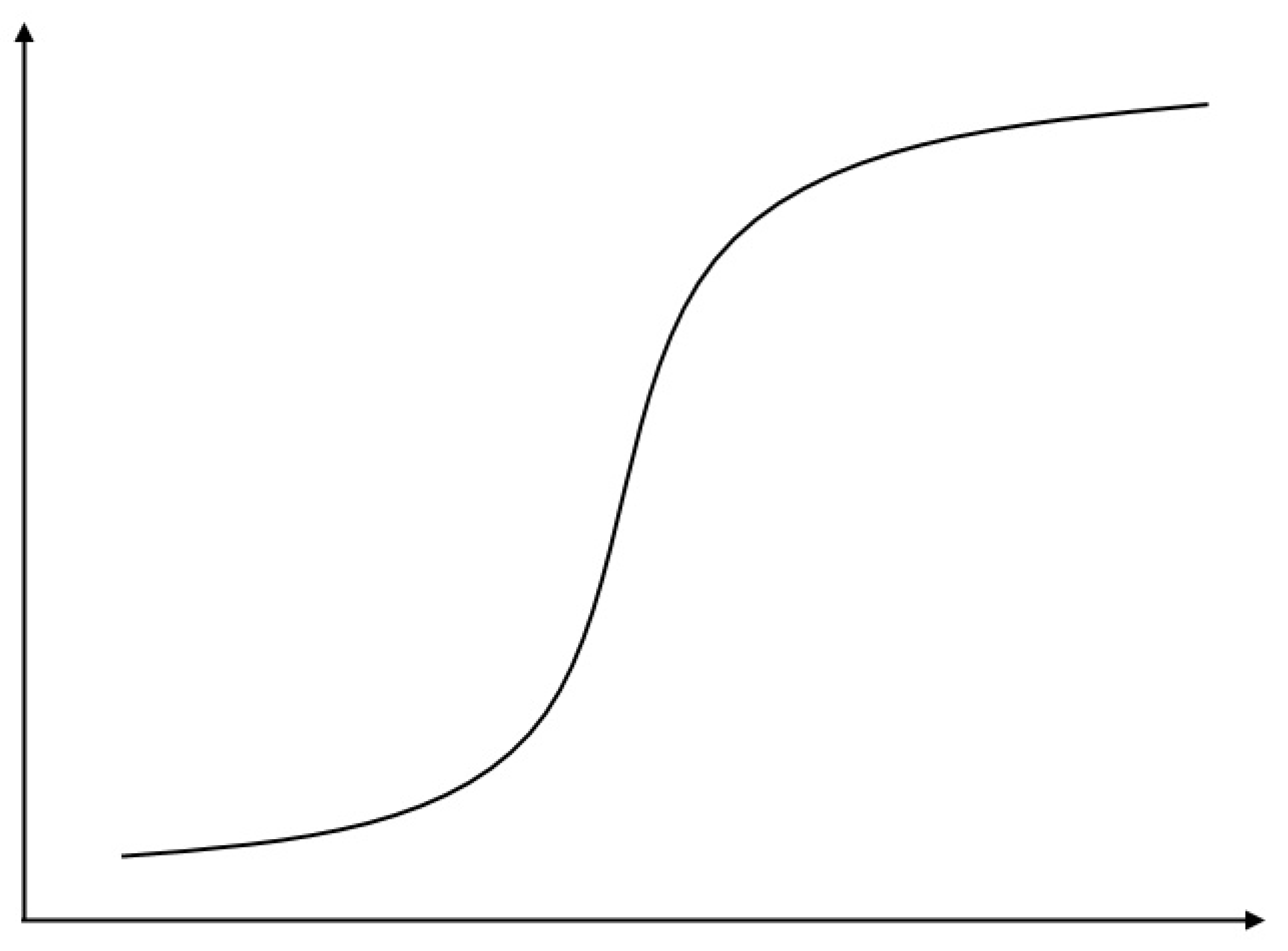
6.4. Characteristic Points for the Curves of the Real-Time PCR

Real-time polymerase chain reaction (real-time PCR, qPCR), based on the PCR method [51], allows you to determine the presence of the target nucleotide sequence in the sample and measure the number of its copies. The amount of amplified DNA is measured after each cycle of amplification using fluorescent labels. Evaluation can be quantitative (measuring the number of copies of the template) and relative (measuring relative to the introduced DNA or additional calibration genes). For real-time PCR, the amount of product formed is monitored during the reaction by monitoring the fluorescence of the dyes introduced into the reaction. The number of fluorophores is proportional to the amount of the resulting DNA product. Assuming a specific amplification efficiency, which is usually close to doubling the number of molecules per amplification cycle, it is possible to calculate the number of DNA molecules initially present in the sample. Thanks to highly efficient detection chemistry, sensitive instrumentation, and optimized analysis methods, DNA molecules can be quantified with unprecedented precision [52].

The fluorescence accumulation curve (fluorescence graph) for real-time PCR has a characteristic form (Figure 6); it consists of a baseline, an exponential phase, and a plateau phase [53].

For initial cycles, when the fluorescent signal is below the value that the instrument can register, the amplification graph slowly increases as a linear function. Then, as the product accumulates, the signal increases exponentially and then reaches a plateau, similar to an arctangent. The plateau is due to the lack of one or another component of the reaction. In a standard real-time PCR reaction, all samples will plateau and reach approximately the same signal level. On the other hand, in the exponential phase, differences in the growth rate of the amount of product can be traced. Differences in the initial number of molecules affect the number of cycles required to raise the fluorescence level above the noise level.

There are many mathematical models describing the fluorescence graph for real-time PCR [54,55]. In some cases, theoretical and practical interest is not a heuristic inference, but a formal determination of the moments of transition of the fluorescence accumulation curve from linear growth to exponential growth, and then, reaching the plateau [56,57].

6.5. Switched Systems

Continuous dynamics and discrete events interconnect many systems encountered in practice. Systems in which these two types of dynamics coexist and interact are usually called hybrid systems. Their study entails interesting theoretical problems that are important for solving many applied problems. Due to its interdisciplinary nature, this field attracts the attention of a wide range of scientists. Researchers with experience and interest in continuous-time systems and control theory are primarily interested in the properties of continuous dynamics, such as Lyapunov stability. At the same time, it is necessary to study the discrete behavior of such systems. To describe the specifics of discrete dynamics, it is helpful to analyze a more general situation that contains a specific model as a particular case. We can is done this by considering systems with continuous-time and discrete switching events from a particular class. Such systems are called switched systems and are considered higher-level abstractions than hybrid systems. It should be borne in mind that such systems often demonstrate non-trivial switching behavior and, thus, go beyond the traditional control theory [58].

For example, we can consider the security issues on the Internet of Things (IoT), which connects devices and users without limiting time and place. Latency, availability, and reliability are critical metrics for the efficient use of IoT data and services. IoT devices equipped with embedded controllers are often targeted by denial-of-service attacks. Denial-of-service (DoS) attacks and Distributed Denial-of-Service (DDoS) attacks are the most common attacks on the Internet of Things [59]. They can take many forms and are defined as attacks that can undermine the network’s ability to perform its function. During DoS and DDoS attacks, several “malicious” computer systems “flood” the selected server with a huge volume of concurrent requests and cause a denial of service for users and devices on the network [60].

In these cases, the system must change “its behavior” depending on the situation and use specialized hardware and software methods to deal with them. A possible approach, in this case, would be to use machine-learning methods in the IoT [61]. The fact is that random functions, which are mappings between the generalized time and the amount of information (the number of requests), at the beginning of the attacks change the character of their increase from linear to nonlinear form, as a rule—exponential (Figure 7). Approximation-estimation tests can be used to definition Markov stopping time corresponding to a change in strategy in response to an attack or overload.

The flexibility of the set of approximation-estimation tests allows them to make decisions on changing the control strategy based on any available metric. Network congestion control can be thought of as a switching system [62,63]. In this case, the primary mechanism for congestion avoidance is to determine the available system bandwidth. If the network is overloaded, it is necessary to automatically switch to emergency mode with a decrease in unacknowledged packets.

One of the most critical aspects of the considered tools is that the decision to change the strategy is made based on data on changes in the nature of network activity and not based on overcoming specific fixed load values. This allows these algorithms to be applied without additional configuration on systems of any size.

7. Conclusions

At the end of the article, it should be noted that modern computers do not learn anything. Typical machine learning boils down to finding and using “mathematical formulas” that produce the desired results when applied to a set of inputs. Just as artificial intelligence is not intelligence, machine learning is not learning. The term was coined for marketing reasons; in the 1960s, IBM used it to attract customers and talents [64]. Nevertheless, the term machine learning has gained worldwide acceptance and is understood as the theory and practice of creating hardware and software that can perform practical actions without direct human intervention.

The practical application of approximation-estimation tests for solid mechanics, molecular biology, and switching systems can be attributed to a particular case of detecting anomalies. The same applies to their use in cluster analysis; the definition of “elbow” on the graph identifies an anomaly. Specific implementations of the proposed formulas and algorithms and an assessment of their computational complexity are beyond the scope of this article, but there are no prerequisites to believe that this aspect will cause significant difficulties in implementation. Moreover, the implementation of algorithms using approximation-estimation tests is possible in both hardware and software.

Approximation-estimation tests and integral-estimation tests open up new purely mathematical problems. For example, we can be studying their extreme properties. Approximation-estimation tests let obtain an upper bound for the critical point of the transition of the trajectory of a quasi-deterministic process from linear to nonlinear growth. Moreover, if the trajectory is convex, then an increase in the approximation knots shifts this upper bound to the left. Integral and differential calculus tools provide more accurate results than discrete methods. Therefore, it can be assumed that integral-estimation tests allow one to obtain more accurate estimates for critical points of monotonic trajectories than approximation-estimation tests. The next problem, by the way, is related to the previous one. Behavior study of approximation-estimation tests and integral-estimation tests if an increasing variable has not one inflection point, such as a sigmoid or a logit, but a countable set of such points, etc.

And in the end, for the sake of fairness, it should still be noted that integral-estimation tests are primarily of academic interest since practical implementation in digital technologies is possible mainly for discrete solutions.