A Goal Programming-Based Methodology for Machine Learning Model Selection Decisions: A Predictive Maintenance Application

Abstract

The paper develops a goal programming-based multi-criteria methodology, for assessing different machine learning (ML) regression models under accuracy and time efficiency criteria. The developed methodology provides users with high flexibility in assessing the models as it allows for a fast and computationally efficient sensitivity analysis of accuracy and time significance weights as well as accuracy and time significance threshold values. Four regression models were assessed, namely the decision tree, random forest, support vector and the neural network. The developed methodology was employed to forecast the time to failures of NASA Turbofans. The results reveal that decision tree regression (DTR) seems to be preferred for low values of accuracy weights (up to 30%) and low accuracy and time efficiency threshold values. As the accuracy weights tend to increase and for higher accuracy and time efficiency threshold values, random forest regression (RFR) seems to be the best choice. The preference for the RFR model however, seems to change towards the adoption of the neural network for accuracy weights equal to and higher than 90%.

1. Introduction

Industry 4.0 has revolutionized business processes and operations as it now provides capabilities for dynamically collecting and managing a vast amount of data from IoT devices [1]. On this basis, software democratization provides an opportunity for efficiently managing these data, with ML models emerging as tools for further facilitating the data and supporting decision-making [2]. These models are trained on a train-dataset and evaluated on a test-dataset to examine their accuracy, with their success hinging upon their ability to dynamically train on data, capture recent disruptions, and thus further provide dynamic forecasts [3].

Artificial Neural networks (ANNs) are types of ML models that are characterized by a complex algorithmic process for prediction, which could in turn lead to more accurate forecasts. This algorithmic complexity leads to significantly high algorithmic training times, especially when the number of features increase [4]. As a result, ANNs lack the potential to be dynamically trained on real-time data, and thus provide dynamic forecasts. This drawback may not allow the planner to identify a potential disruption on-time and thus take appropriate proactive actions.

On the other hand, advanced regression models such as DTR, RFR and support vector regression (SVR) are ML models, whose solution process is simpler. This simplicity allows for dramatically reduced training times that provide users with the capability to dynamically train the model to datasets retrieved on a real time basis, and further deliver dynamic forecasts [5]. However, the simplicity in the algorithmic process could in turn lead to less accurate forecasts.

Predictive maintenance (PdM) is condition-based research field, that heavily depends on dynamic data of equipment and sensors. It does not substitute the traditional periodic maintenance management relying on routine servicing and run-to-failure programs but makes it more reliable by providing a scheduling tool for dynamic PdM tasks [6]. The dynamic monitoring of the operating condition of machines and the resulting dynamic estimation of their mean time to failure, results in the following: (i) reductions of unnecessary maintenance operations, (ii) increase in the time that spare parts are used, (iii) prevention of unexpected machine breakdowns and (iv) increases of the available production times [7].

ML models ability to handle a large stream of data from IoT sensor devices is one of the main drivers that support their utilization for PdM [8]. However, and based on [8], two critical challenges emerge and involve the following: (i) the latency associated to the high dynamic training times of the ML models as these derive from the need for real-time monitoring of large machine operating condition data streams and (ii) the selection of the ML algorithm that better fits to a specific scenarios.

On this basis, the purpose of this paper is twofold. Firstly, to address the above challenges, through the development of a fast, computationally efficient and user-friendly goal programming-based methodology that allows planners to (i) select the ML algorithm that balances prediction accuracy and training time efficiency and (ii) assess ML models in a time efficient manner, for different accuracy and time significance weights as well as accuracy and time significance threshold values, thus providing planners with the flexibility to quantify the impact of higher and lower latencies on prediction accuracy and further identify solutions more appropriate for different scenarios. Secondly, it allows planners to illustrate the applicability of the developed methodology in a real-world PdM problem and derive critical managerial insights for predicting remaining lifetimes of machines and equipment.

The rest of the paper is organized as follows. Section 2 provides a critical synthesis of the existing state of the art literature review on PdM and ML algorithms, while in Section 3, the goal programming-based methodology is provided for selecting the best ML model, along with an analysis of the ML models that will be examined. Section 4 describes the numerical analysis process, while Section 5 analyzes the results. Finally, Section 6 wraps ups with the discussion and conclusions.

2. Literature Review

There is a large number of the PdM methods (e.g., vibration monitoring, thermography, ferrography, acoustic emission, corrosion monitoring etc.) [9] that include the monitoring and measuring of different process parameters and generate a big volume of data, e.g., actual machine condition, failed components, failure rate, mean-time-between-failures, repair times. This data is collected by different real-time and offline sources and can be used to predict the future trends of the machines, to schedule and plan disruptions and the required repairs in most cost-effective time point [10]. Moreover, such massive input of data could benefit from implementation of machine intelligence in maintenance modeling and management addressing the needs of the Industry 4.0 and building an intelligent manufacturing [11]. Zonta et al. (2020) [1] classify three main approaches used for prediction, namely physical model-based, knowledge-based and data-driven, where the last one includes models based on ML algorithms.

ML models are characterized by the ability to deal with a large amount of multivariate data and the learning capability of algorithms. Due to this fact, ML is an appropriate tool in PdM, and currently it is being increasingly applied to PdM. There is a number of predictive algorithms that used in ML where each type represents its own patterns and has a bearing upon the performance of PdM applications. Carvalho et al. (2019) [12] ranked ML algorithms by the extent of application in PdM, detecting that Random Forest (RF) algorithm [13] is used most frequently, followed by Decision Tree (DT) [14], ANNs based methods [15], Support Vector Machine (SVM) [16], k-Nearest Neighbor (KNN) [17], Linear Discriminant Analysis (LDA) [18] and Bayesian Network [19]. These algorithms can perform prediction tasks or validate proposed plans. In most cases, the PdM models are developed with the use of real vibration data. However, manufacturing plants are dynamic units where the processes change dynamically. This fact causes the heterogeneity of the data and can affect the predictability of the ML models. Due to these two aspects there is no universal model that could be applied to different scenarios [19]. Besides, each ML algorithm has its specific characteristics and applications.

Examples of the papers that use the aforementioned algorithms include [20], where the authors create a PdM experiment setup for the detection of the faulty bearing based on IoT. They model the obtained data with the use of five ML algorithms, namely SVM, LDA, RF, DT, and KNN and evaluate the models with the use of eight different metrics. Syafrudin et al. (2018) [21] propose a real-time monitoring system that utilizes IoT-based sensors, big data processing, and a hybrid model for fault detection in order to improve decision-making for automotive manufacturing. This prediction model utilizes density-based spatial clustering of applications with noise to separate outliers from normal sensor data, and RF classification to predict faults. Ali et al. (2019) [22] provide a software middleware that uses the outcomes of real-time data analytics in combination with ML models trained over historical data for production forecasting within a manufacturing unit in real-time. The authors apply regression-based approaches for prediction such as Multiple Linear Regression, SVR, DTR and RFR. The proposed integrated framework allows one to calculate the impact of detected abnormal events and set the optimal production targets accordingly. In the context of real-time decision making, [8] high levels of Scalability and network Bandwidth both are the compulsory requirement and one of the major challenge for applying ML models in PdM. Liu et al. (2018) [23] address this issue by proposing training of ML models at the edge of the networks for real-time feature extraction and anomaly detection of the high-speed railway transportation system. The proposed methodology incorporates Auto-Associative Neural Network.

ANNs technique is widely used by the authors to tackle issues related to PdM. Li, et al. (2017) [24] point out that the main benefits of ANNs are fault tolerance, generalization and adaptability, at the same time, the lack of an explanation function is identified as a limitation. The authors apply ANNs for fault prediction, focusing on the prognosis process for a backlash error in machine centers. Crespo et al. (2019) [25] combine ANNs with data mining to address the problem of assets’ performance monitoring predicting any loss of energy consumption efficiency, where ANNs is used to identify when asset behavior abnormalities can appear. Daniyan, et al. (2020) [26] develop the training modules comprising ANNs with dynamic time series model to predict the state and potential failure of a railcar wheel bearing. Recurrent Neural Networks (RNN) technique is a type of ANNs that is also implemented to deal with PdM problems and is characterized by the ability to capture the dynamics of sequence data [27]. For example, [28] create Long Short-Term Memory model using RNN to predict failures and to estimate the number of remaining cycles or Remaining Useful Life. Bogojeski et al. (2021) [29] also invoke the use of RNN technique to model the industrial aging process forecasting problem in the context of predicting degradation of chemical process equipment.

Moreover, some processes may demand the combination of ML techniques. Huang et al. (2020) [30] deal with multi-source sensing data fusion models and algorithms based on neural network in mechanical equipment fault diagnosis and prediction. The authors come to conclusion that the mentioned algorithms need to be combined with data preprocessing algorithms (e.g., SVM) to achieve higher accuracy. A number of authors apply a combination of both ANNs and SVM techniques. Thus, [27] bring together these techniques to predict the machine systems’ failure events through monitoring the cutting tool and the spindle motor, where SVM was used to classify the conditions of the cutting tool, while two ANNs algorithms were used to monitor the condition of bearing. The study of [31] focuses on the development of framework that can prevent the failure and extend the lifetime of mechanical, electrical and plumbing components of building facilities. The results show that the proposed model that combines ANNs and SVM techniques can efficiently predict the future condition of these components for maintenance planning. Besides this combination, [32] develop a PdM approach towards an early warning maintenance/failure warning system for floating dock ballast pumps using MATLAB and SVM algorithm. Gohel et al. (2020) [33] combine SVM and logistic regression algorithms to perform PdM of nuclear infrastructure and to predict the failure of nuclear plant infrastructure and engines.

Çınar et al. (2020) [34] reviewed the number of papers on the application of ML algorithms in PdM that were published between 2010 and 2020. The authors came to the conclusion that a single prediction method may not provide best results, and the combination of more than one ML model could provide more accurate prediction. The accurate multi-criteria decision making methodology for recommending ML algorithm was provided by [35], which evaluates and ranks classifiers’ and helps to learn and build classification models and includes criteria selection method, relative consistent weighting scheme, a ranking method, statistical significance and fitness assessment functions, and implicit and explicit constraints satisfaction at the time of analysis. The performance evaluation of ML algorithms using multi-criteria decision making techniques was also discussed by [36] who applied Fuzzy Analytical Hierarchical Process (FAHP) in assigning weights to the criteria and ranking the performance criteria and implemented Simple Additive Weighting and TOPSIS model to rank the classifiers for comparison. While [37] proposed a library-based overview regarding component security evaluation based on multi-criteria decision and ML algorithms. Earlier, [38] developed a multi-criteria–based active learning approach to apply it to named entity recognition.

A summary of the related research in the realm of ML techniques in PdM is presented in

Table 1. Literature review.

References	Focus Area/ Case Study	ML Model	Optimization Criteria	Methodology Used	Decisions
[20]	PdM for the detection of the faulty bearing	SVM, LDA, RF, DT, and KNN	Accuracy, precision, TPR, TNR, FPR, FNR, F1 score and, Kappa metrics	Statistical (resampling) methods, cross-validation approach	ML models performance evaluation
[21]	Real-Time Monitoring System/ automotive manufacturing assembly line	Hybrid prediction model: Density-Based Spatial Clustering of Applications with Noise-based outlier detection RF classification	Fault prediction accuracy	Comparison of the hybrid prediction model with other classification models (NB, LR, MLP, RF)	Fault detection
[22]	Production forecasting/ Biomedical devices manufacturing	Regression-based approaches (MLR, SVR, DTR and RFR)	Scrap, Rework, Lead Time and Output	Semantically interoperable framework, Root Mean Square Error mechanism	Predictions about future production goals, abnormal events detection
[23]	PdM/High-speed railway transportation system	Auto-Associative Neural Network (AANN)	Vibration and speed relationship	Training of ML models at the edge of the networks	Potential faults prediction
[24]	PdM/Machine Centers	ANNs	Backlash error	Training and prediction process	Fault prediction
[25]	Asset performance monitoring/energy plants and facilities	ANNs with Data Mining tools (Association Rule Mining)	Behavior abnormalities	Combination of ANNs and Association Rule mining approaches	Prediction of any loss of energy consumption efficiency
[26]	PdM/railcar wheel bearing	ANN with dynamic time series model	Wheel-bearing temperature	Levenberg Marquardt algorithm	Failure prediction
[27]	PdM/machine tool systems	SVM, ANN (RNN and CNN)	Prediction accuracy	Confusion matrix	Failure prediction
[29]	Industrial aging process/chemical plant	Linear and kernel ridge regression (LRR and KRR), feed-forward neural networks, RNN (echo state networks and long short term memory networks)	Degradation KPIs	Training of ML models and model comparison	Predicting a KPI
[31]	PdM/building maintenance management	ANNs, SVM	The condition index of MEP components in buildings, triggers and alarms for the required maintenance actions	Training of ML models and algorithms comparison	Future condition of MEP components
[32]	PdM/floating dock ballast pumps	SVM	Principle components, e.g., PC1–flow rate and PC2–suction pressure	Principal component analysis (PCA)	Maintenance/failure prediction
[33]	PdM/Nuclear infrastructure	SVM, logistic regression algorithms	State of an engine, scoring	Confusion matrix	Failure prediction
[35]	-	Multi-class classification algorithms	Accuracy, computational complexity, and consistency	AMD methodology, Wgt.Avg.F-score, CPUTimeTesting, CPUTimeTraining, and Consistency measures, TOPSIS method	-
[36]	-	Bayes Network, Naive Bayes, LR, Sequential Minimal Optimization, Multilayer Perceptron, Tree and Lazy (Instance Based Learner)	Performance Metrics, Criteria weights	Multi-criteria–approach, FAHP and TOPSIS model	-
[38]	Named entity recognition	SVM	Informativeness representativeness and diversity	Multi-criteria -based active learning approach	To minimize the human annotation efforts
This paper	PdM/prediction of the lifetime of aircraft engines	ANNs and Regression models (SVR, the DTR and the RFR)	Forecasting accuracy, time accuracy	Multi-criteria–approach, Goal programming	ML model selection

.

The results of the critical synthesis reveal the following:

• To our knowledge there seems to be a small number of research efforts that provide a multi-criteria decision-making methodology for ML algorithm selection.
• The aforementioned research efforts provide time consuming multicriteria methodologies, are theoretical in nature and cannot be easily adapted to multiple scenarios as the weights assigned to ML selection criterions are a result of a time-consuming statistical process. Moreover, they do not relate to any focus areas or case studies, and their applicability in PdM is not demonstrated.

This paper contributes to the existing literature through the following:

• Development of a multi-criteria decision-making methodology for ML model selection that utilizes the method of Goal Programming. The methodology allows for undertaking a time-efficient sensitivity analysis process of the weights assigned to the criteria, and of the criteria threshold values, thus providing the decision maker with a wide range of alternatives for optimal ML model selection that make the model suitable for multiple PdM scenarios where the weights on time and accuracy efficiency maybe different.
• Assessment of the model’s applicability on the real-world dataset of NASA Turbofans time to failures and the generation of practical managerial insights for predicting the remaining lifetimes of machines and equipment.

3. Materials and Methods

The methodological approach employed involves the development and assessment of different type of ML models $m \in M$ for the forecasting of a machine’s time to failure. The employed models will be fitted in a training dataset and employed to forecast the dependent variable value of a test dataset. The forecasting accuracy of the models is denoted by $a_i$ and will be assessed by the Mean Absolute Percentage error (MAPE) metric, thus ranging from 0 to 100%, while the time efficiency, by the models total training and error generation times, denoted by $t_m$.

In order to find the best model that balances time efficiency and model accuracy, a goal programming-based methodology will be employed. Thus, significance weights on forecasting accuracy and time efficiency will be set, denoted by $w_a$, and $\left(1-w_a\right)$, respectively and the best model selected should lead to the lowest value of the following deviation function $d_m$.

$$d_m=w_a·\left(\frac{a^{*}-a_m}{a^{*}}\right)+\left(1-w_a\right)·\left(\frac{t_m-t^{*}}{t^{*}}\right), \forall m\in M$$

(1)

where $a^{*}, t^{*}$ represent target accuracy and time efficiency values respectively. Thus, and as the accuracy values tend to increase and the training and error generation times decrease, the deviation function value is constantly being reduced.

The nomenclature of the model parameters are summarized in the following

Table 2. Nomenclature of the deviation function parameters.

$w_a, \left(1-w_a\right)$	Significance weights assigned to the models forecasting accuracy and time efficiency respectively
$a_m$	$\mathrm{Forecasting} \mathrm{accuracy} \mathrm{value} \mathrm{of} \mathrm{the} \mathrm{ML} \mathrm{model} m\in M$ (0–100%)
$t_m$	$\mathrm{Training} \mathrm{and} \mathrm{error} \mathrm{generation} \mathrm{time} \mathrm{of} \mathrm{the} \mathrm{ML} \mathrm{model} m\in M$ (time units)
$a^{*}, t^{*}$	Fixed target accuracy and time value thresholds (0–100%) set by the planner

:

Four regression models will be examined, namely the SVR, the DTR, the RFR, and the neural network regression.

3.1. Support Vector Regression (SVR)

The method considers a number of independent variables $i \in I$, of a training set denoted by $x_i$, and their respective weights denoted by $w_i$. For mathematical expression simplicity, [39] expresses the independent variables $x_i,$ as a vector $x$ and the weights assigned to the independent variables $w_i,$ as a vector $w$. These are then used for determining the hyperplane line equation function of Equation (2), where b corresponds to the hyperplane bias.

$$f\left(x\right)=w·x+b,$$

(2)

The hyperplane line splits the independent variable space in two regions. The first region involves the area above the line $f\left(x\right)=1$, and is denoted by $R^{+}$, while the second one, by the area below the line $f\left(x\right)=-1$ and is denoted by $R^{-}$. This type of split does not consider the independent variable values of the training set between these two lines, when determining the optimal values of $w,b$ thus providing higher degrees of freedom of the model and the flexibility to derive lower forecasting error potential for a test set [40].

The distance of the hyperplane line from $f\left(x\right)=1$, is denoted by $d^{+}$ and from $f\left(x\right)=-1$, by $d^{-}$. The sum of these distances can be estimated as $2·\left(\frac{w·x+b}{\Vert w\Vert }\right)$, where $w$ corresponds to the length of the weight vector $w$. The optimization function and the model’s constraints are summarized below [41].

$$\begin{array}{c}Ma{x}_{w,b}\left[2·\left(\frac{w·x+b}{\Vert w\Vert }\right)\right]\\ Subject to \{\begin{array}{c}w·x+b\ge 1 for x_i\in R^{+}\\ w·x+b\le -1 for x_i\in R^{-}\end{array}\end{array}$$

(3)

3.2. Decision Tree Regression (DTR)

DTR is a tree-structured regression model, normally using mean squared error on deciding how to optimally split a node in two or more sub-nodes [42].

As in the SVR model, $x_i$ represents the values of the independent variables $i\in I$, of the training set and $y_i$, the corresponding values of the dependent variables. The model aims to determine the optimum number of split variables $j\in J$, denoted by $s_j$, and split points $p\in P$, denoted by $s_p$, that minimize the number of binary partitions of a region, denoted by, $R_1^{s_j, s_p },$ $R_2^{s_j, s_p },$ under the sum of mean square error minimization objectives [41]. The model’s optimization function is presented through the following Equation (4) [43].

$$mi{n}_{s_j,s_p}\left[mi{n}_{c_1}{\displaystyle \sum }_{x_i\in R_1^{s_j, s_p }}{\left( y_i-c_1\right)}^2+{\displaystyle \sum }_{x_i\in R_2^{s_j, s_p }}{\left( y_i-c_2\right)}^2\right],$$

(4)

where, $c_1,c_2$, correspond to the average values of the $y_i$ variables corresponding to the $x_i$ of each partitioned region as presented below through Equations (5) and (6):

$$c_1=ave\left(y_i|x_i\in R_1^{s_j, s_p }\right)$$

(5)

$$c_2=ave\left(y_i|x_i\in R_2^{s_j, s_p }\right)$$

(6)

3.3. Random Forest Regression (RFR)

Compared to DTR, the RFR model generates multiple decision trees, by randomly selecting a sample of the independent variables $x_i$ and their respective variables $y_i$, from the examined dataset. For each decision tree, the model optimizes the same decision variables $s_j, s_p,$ as in those optimized under the DTR model, and under the sum of mean square error minimization objectives. An additional decision variable is considered, and involves the number of random (ensemble) trees $e\in E$, that the RFR should generate, determined under average mean square error minimization objectives [44]. The derived forecasted value of the RF is then estimated as an average value of the forecasts of the randomly selected decision trees.

3.4. Artificial Neural Networks (ANNs)

Based on [45], the neural network consists of input layers that are connected with hidden layers, and the hidden layers are in turn connected with output layers. During the training process the independent variable values $x_i$ are used, as inputs to neuron and are distributed unchanged between the input and the hidden layers.

Between the hidden and the output layer though, the inputs are transformed to a weighted sum further reduced by a threshold value of the neuron, denoted by $o_i$, as presented in the following Equation (7):

$$x_j={\displaystyle \sum }_{i\in I}{w}_{ij}·x_i-{\theta }_j,\forall j\in J,$$

(7)

where $w_{ij},$ corresponds to the weight assigned to the independent variable of the input layer $i$ that is distributed to the hidden layer $j$, and ${\theta }_j$ corresponds to the threshold value of layer $j$.

The results of the output layer are then expressed as a non-linear function of $x_i,$ and through Equation (8) as follows:

$${\overline{y}}_j=f\left(x_j\right)={\left[1+e^{-x_j}\right]}^{-1}$$

(8)

The algorithm’s objective during the training process is to determine the optimal values of ${\theta }_j, w_{ij}$ that minimize the mean square errors $E_p$, per training pattern $p\in P$, through Equation (9) [45]:

$$Mi{n}_{{\theta }_j, w_{ij} }\left(E_p\right)=Mi{n}_{{\theta }_j,w_{ij} }0.5·{\displaystyle \sum }_{p\in P}{\displaystyle \sum }_{j\in J}{\left({\overline{y}}_{pj}-y_{pj}\right)}^2$$

(9)

4. Numerical Analysis

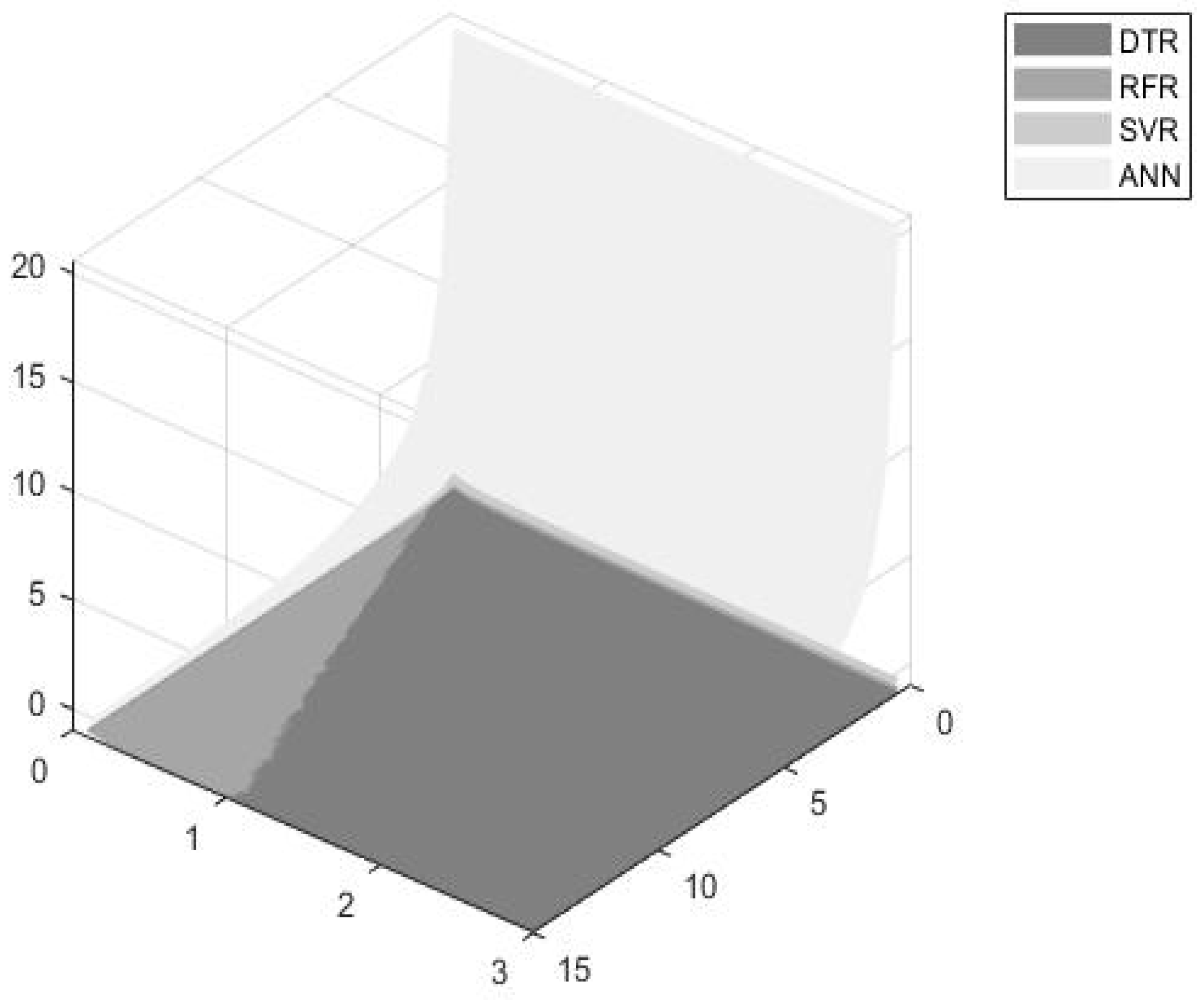
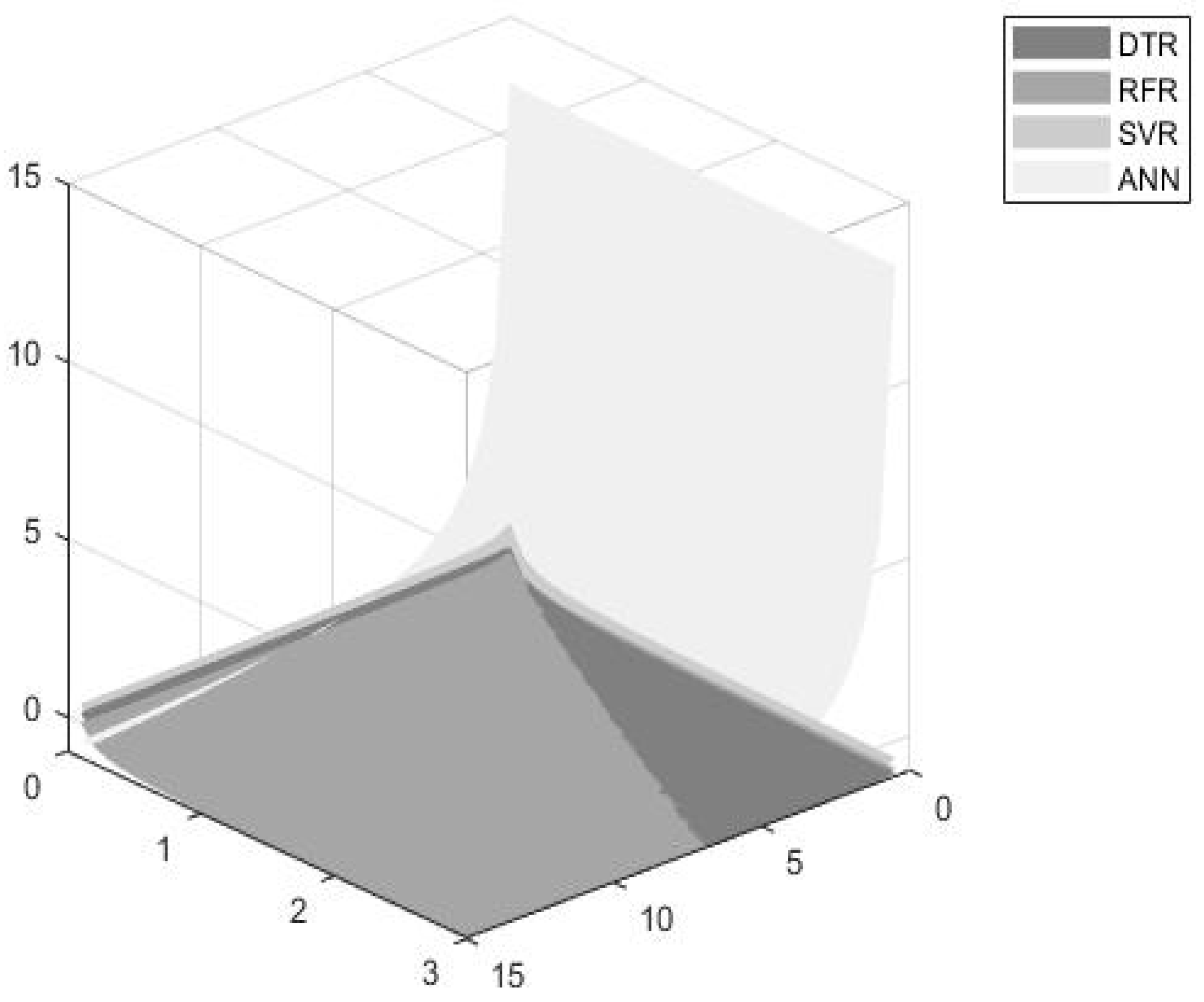
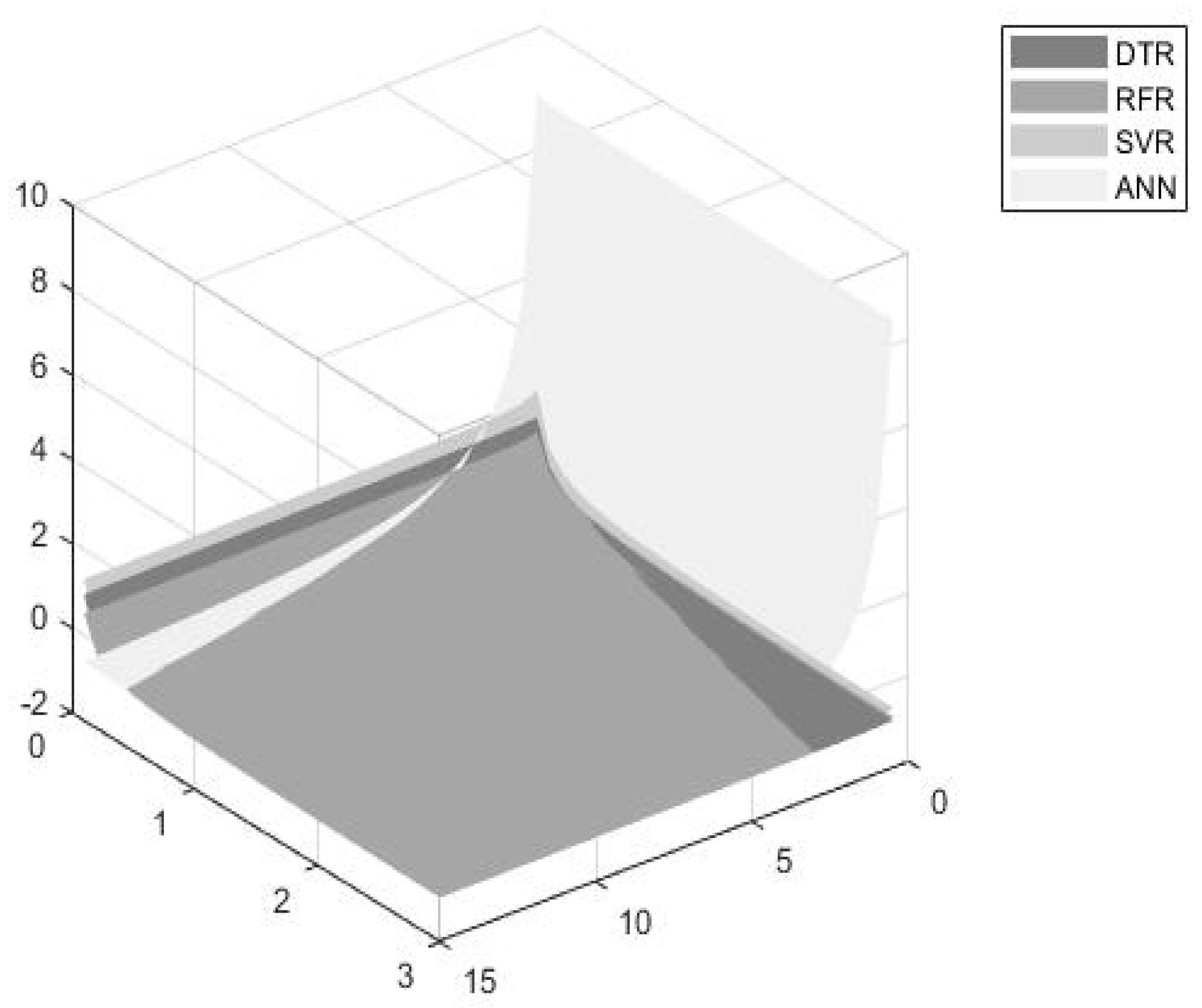
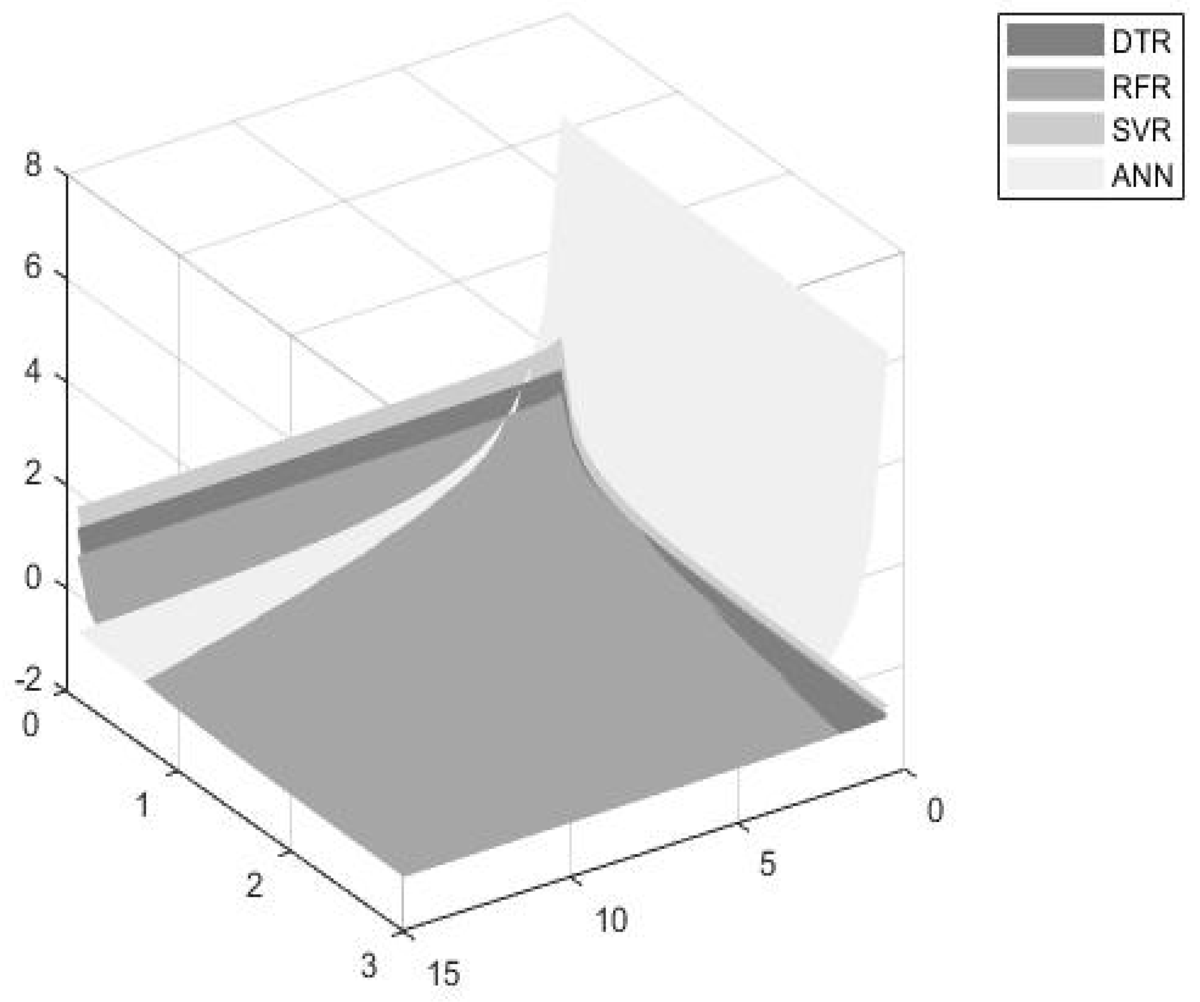
The applicability of the developed methodology will be examined through its application in the Turbofan Engine Degradation Simulation Data Set provided by the Prognostics CoE at NASA Ames [46]. The dependent variable involves the number of the turbine times to failure, while the independent variables involve three operational settings, 26 sensor measurements and the Turbofans unit numbers.

The examined models will be trained on a training set and employed for the forecasting of the test set using Spyder (Python 3.8). The training and forecast times will be captured along with the derived mean square errors for each model type. A sensitivity analysis will be conducted for the accuracy and time significance weights denoted by $w_a, \left(1-w_a\right)$ respectively, and on the target accuracy and time values, denoted by $a^{*}, t^{*}$ respectively.

The accuracy and time significance weights will range from 10 to 100% with a step of 10%. The sensitivity analysis of the target accuracy threshold will start from 0.1% to 3% with a step of 0.1, while the sensitivity analysis of the time efficiency threshold from 1 to 15 min with a step of 0.5 min.

5. Results

The results of the forecasting process for each model type are summarized in

Table 3. Accuracy and time performance characteristics of the examined methods.

Model	$\mathbf{MAPE} ({\mathit{a}}_{\mathit{i}}) \%$	$\mathbf{Time} ({\mathit{t}}_{\mathit{i}}) \mathbf{mins}$
DTR	0.329	0.07
RFR	0.253	0.19
SVR	0.388	0.42
ANN	0.011	10.00

. For all models an 80% training set was considered. An attribute selection process was employed for the regression models leading to only 4 out of 25 important decision variables, namely the Turbofan’s, unit number and the results of sensors 4, 9 and 11. Moreover and specifically for the ANN regression model, a Keras regressor was employed, with a significantly low MAPE value realized after 1000 training epochs.

Based on the formulated Table, we observe that the ANN model exhibits the best performance in terms of accuracy; however, the time required is extremely high in order to allow for a dynamic training process, which could in turn lead to a lower accuracy in a dynamic setting. On the other hand, DTR is the most time efficient model.

The following graph (Figure 1) depicts the impacts of a sensitivity analysis on the accuracy and time efficiency weights and thus, on the derived deviation functions of Equation (1), while considering a threshold MAPE value of 3% and a threshold time efficiency value of 15 min. The results indicate that the DTR is the most preferable model for accuracy weights ranging from [0.1, 0.3). The RFR is preferable for accuracy weights ranging (0.3, 0.8], while finally, the NN is preferred for accuracy weights ranging from [0.9, 1].

The following Figure 2, Figure 3, Figure 4, Figure 5, Figure 6, Figure 7, Figure 8, Figure 9 and Figure 10 illustrate the results of the sensitivity analysis on accuracy and time threshold values, given fixed values of accuracy weights ranging from 0.1 to 0.9 and thus, of respective time efficiency weights ranging from 0.9 to 0.1.

More specifically, Figure 2 clearly illustrates the prevalence of DTR for almost all of sensitivity analysis values of the accuracy weights. The prevalence is also high in Figure 3, but not in Figure 4, where RFR seems to be the most preferred algorithm. The preference seems to increase further for higher accuracy and time threshold values (Figure 4, Figure 5, Figure 6, Figure 7, Figure 8 and Figure 9), further validating the results of Figure 1, where RFR is preferred for accuracy weights equal to and above 30%.

Another interesting finding involves the gradual preference on ANNs, as the accuracy weights increase, and for higher accuracy threshold values (Figure 4, Figure 5, Figure 6, Figure 7, Figure 8 and Figure 9), with the ANNs prevalence realized, for accuracy weights equal to and above 90% regardless of the sensitivity analysis values on accuracy and time thresholds (Figure 10).

6. Discussion and Conclusions

We developed a fast and computationally efficient methodology for assessing ML algorithms, considering two criteria, namely accuracy and time efficiency. The accuracy is quantified through the MAPE metric, time efficiency, through the algorithms’ training and error generation times.

The methodology is based on goal programming and provides to the user the flexibility to easily assess the models under alternative accuracy and time efficiency weights, and for various values of accuracy and time efficiency thresholds. The methodology was employed for estimating the time to failure of turbofans. The decision tree, random forest, support vector and the neural network regression ML models were examined. The results of the numerical analysis are summarized below:

○

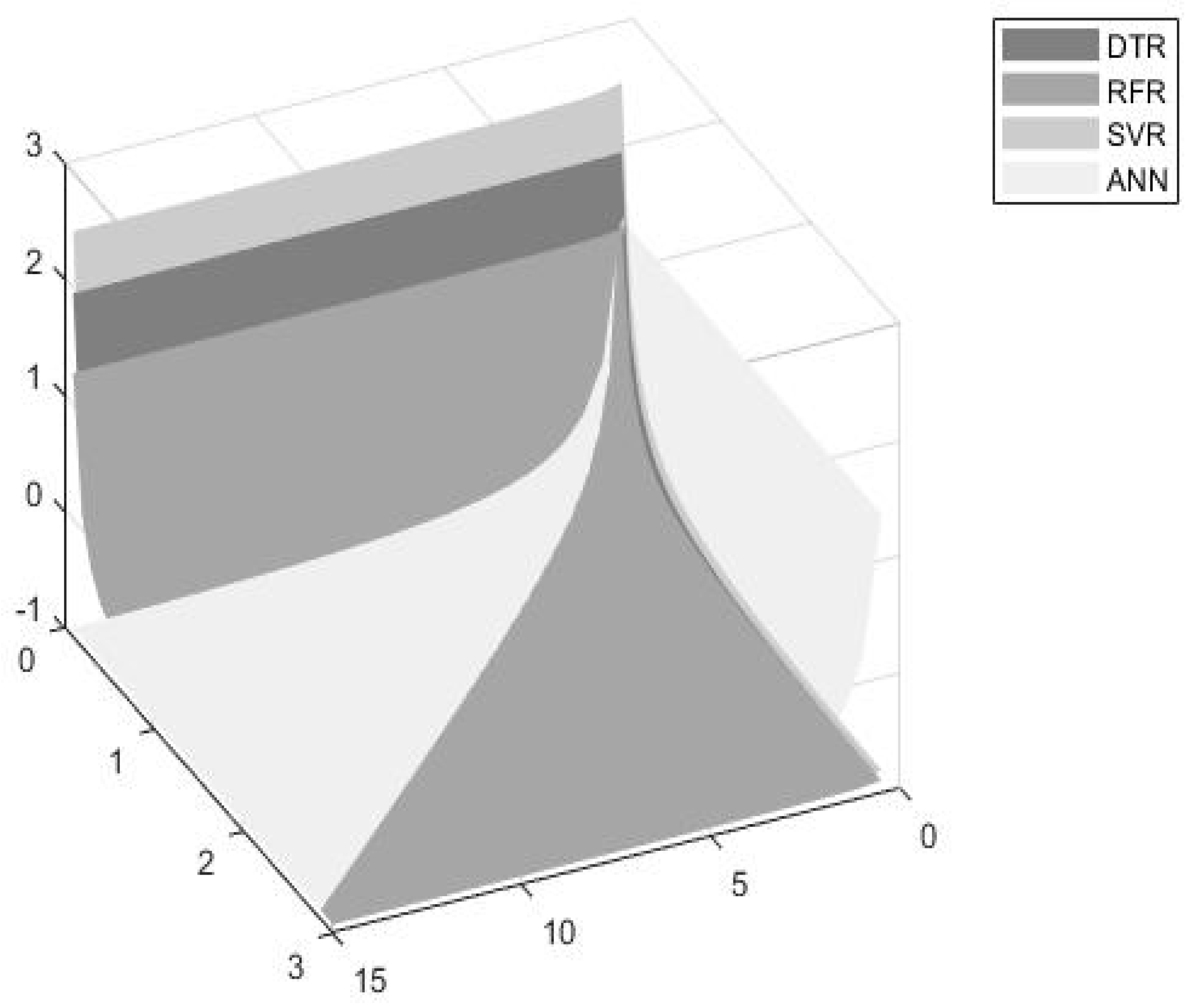
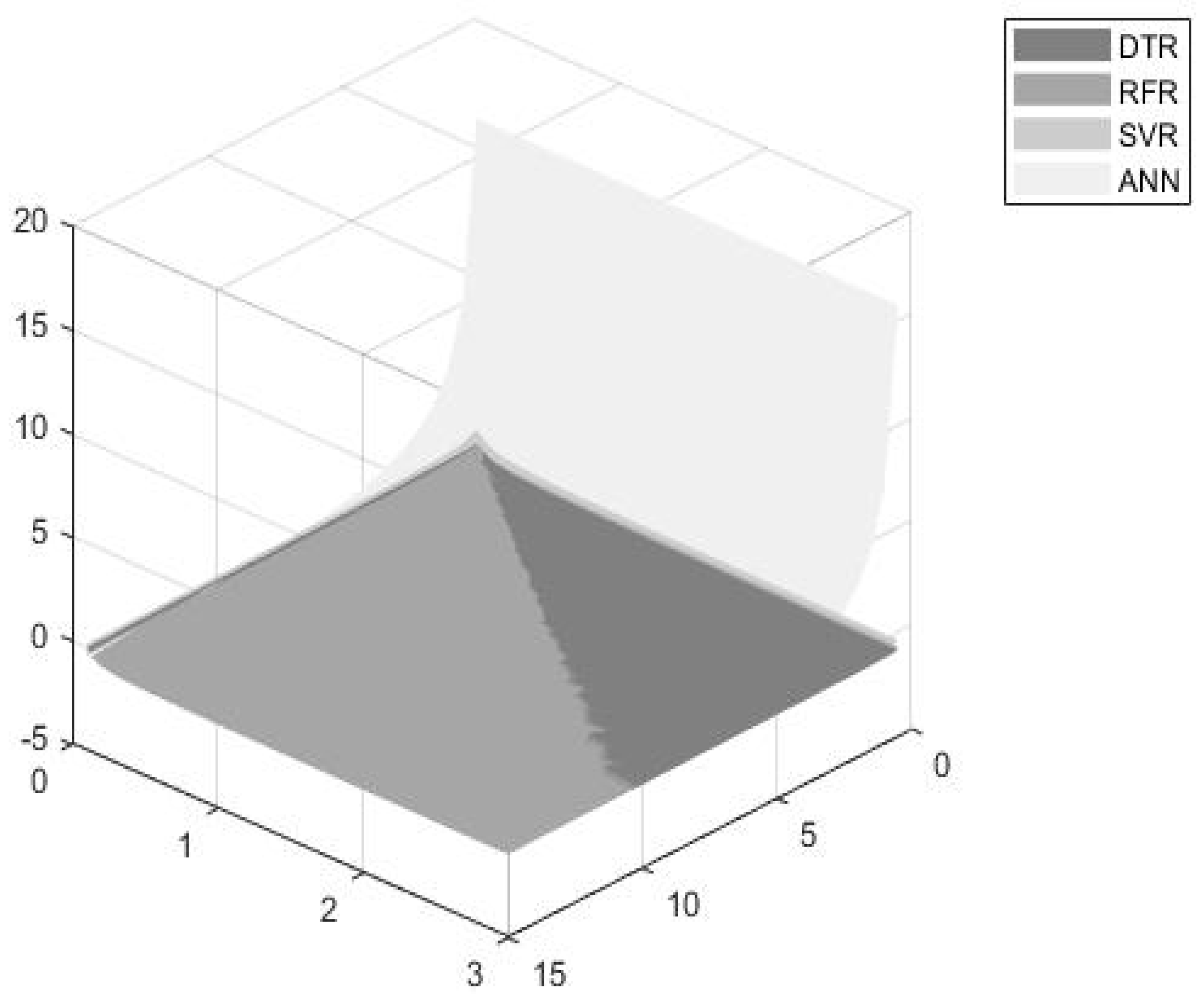
The DTR model seems to be the most efficient model for dynamically estimating turbofan time to failures when considering an accuracy significance weight up to 30%. However, the model’s efficiency seems to decrease as the accuracy and time thresholds increase.

○

The RFR seems to be more efficient for accuracy weights ranging from 30% to 90%, and for higher accuracy and time threshold values.

○

The ANN model exhibits significantly high accuracy values and thus, seems to be more preferable for accuracy weights ranging from 90% to 100%.

References

1. Zonta, T.; da Costa, C.A.; da Rosa Righi, R.; de Lima, M.J.; da Trindade, E.S.; Li, G.P. Predictive Maintenance in the Industry 4.0: A Systematic Literature Review. Comput. Ind. Eng. 2020, 150, 106889. [Google Scholar] [CrossRef]
2. Patel, J. The democratization of machine learning features. In Proceedings of the 2020 IEEE 21st International Conference on Information Reuse and Integration for Data Science (IRI), Las Vegas, NV, USA, 11–13 August 2020; pp. 136–141. [Google Scholar]
3. Samsonov, V.; Enslin, C.; Lütkehoff, B.; Steinlein, F.; Lütticke, D.; Stich, V. Managing disruptions in production with machine learning. In Proceedings of the 1st Conference on Production Systems and Logistics (CPSL 2020), Stellenbosch, South Africa; pp. 360–368.
4. Cavallaro, L.; Bagdasar, O.; De Meo, P.; Fiumara, G.; Liotta, A. Artificial Neural Networks Training Acceleration through Network Science Strategies. Soft Comput. 2020, 24, 17787–17795. [Google Scholar] [CrossRef]
5. Gęca, J. Performance comparison of machine learning algorithms for predictive maintenance. Inform. Autom. Pomiary Gospod. Ochr. Środowiska 2020, 10, 32–35. [Google Scholar] [CrossRef]
6. Mobley, R.K. Plant Engineer’s Handbook; Elsevier Science & Technology: Oxford, UK, 2001; ISBN 978-0-7506-7328-0. [Google Scholar]
7. Einabadi, B.; Baboli, A.; Ebrahimi, M. Dynamic Predictive Maintenance in Industry 4.0 Based on Real Time Information: Case Study in Automotive Industries. IFAC-PapersOnLine 2019, 52, 1069–1074. [Google Scholar] [CrossRef]
8. Dalzochio, J.; Kunst, R.; Pignaton, E.; Binotto, A.; Sanyal, S.; Favilla, J.; Barbosa, J. Machine Learning and Reasoning for Predictive Maintenance in Industry 4.0: Current Status and Challenges. Comput. Ind. 2020, 123, 103298. [Google Scholar] [CrossRef]
9. Girdhar, P.; Scheffer, C. Predictive maintenance techniques. In Practical Machinery Vibration Analysis and Predictive Maintenance; Elsevier: Amsterdam, The Netherlands, 2004; pp. 1–10. [Google Scholar]
10. Thomas, E.; Levrat, E.; Iung, B.; Monnin, M. ‘ODDS Algorithm’-based ipportunity-triggered preventive maintenance with production policy. In Fault Detection, Supervision and Safety of Technical Processes 2006; Elsevier: Amsterdam, The Netherlands, 2007; pp. 783–788. [Google Scholar]
11. Wang, J.; Liu, C.; Zhu, M.; Guo, P.; Hu, Y. Sensor data based system-level anomaly prediction for smart manufacturing. In Proceedings of the 2018 IEEE International Congress on Big Data (BigData Congress), San Francisco, CA, USA, 2–7 July 2018; pp. 158–165. [Google Scholar]
12. Carvalho, T.P.; Soares, F.A.A.M.N.; Vita, R.; da Francisco, R.P.; Basto, J.P.; Alcalá, S.G.S. A Systematic Literature Review of Machine Learning Methods Applied to Predictive Maintenance. Comput. Ind. Eng. 2019, 137, 106024. [Google Scholar] [CrossRef]
13. Strobl, C.; Malley, J.; Tutz, G. An Introduction to Recursive Partitioning: Rationale, Application, and Characteristics of Classification and Regression Trees, Bagging, and Random Forests. Psychol. Methods 2009, 14, 323–348. [Google Scholar] [CrossRef] [Green Version]
14. Salin, E.D.; Winston, P.H. Machine Learning and Artificial Intelligence An Introduction. Anal. Chem. 1992, 64, 49A–60A. [Google Scholar] [CrossRef]
15. Schmidhuber, J. Deep Learning in Neural Networks: An Overview. Neural Netw. 2015, 61, 85–117. [Google Scholar] [CrossRef] [PubMed] [Green Version]
16. Abbas, A.K.; Al-haideri, N.A.; Bashikh, A.A. Implementing Artificial Neural Networks and Support Vector Machines to Predict Lost Circulation. Egypt. J. Pet. 2019, 28, 339–347. [Google Scholar] [CrossRef]
17. Blömer, J.; Lammersen, C.; Schmidt, M.; Sohler, C. Theoretical analysis of the k-means algorithm—A survey. In Algorithm Engineering: Selected Results and Surveys; Springer: Cham, Switzerland, 2016; Volume 9220, pp. 81–116. [Google Scholar]
18. McLachlan, G.J. Discriminant Analysis and Statistical Pattern Recognition; A John Wiley & Sons, Inc. Publication: Hoboken, NJ, USA, 2004; ISBN 978-0-471-69115-0. [Google Scholar]
19. Ansari, F.; Glawar, R.; Sihn, W. Prescriptive Maintenance of CPPS by Integrating Multimodal Data with Dynamic Bayesian Networks. Mach. Learn. Cyber Phys. Syst. Technol. Intell. Autom. 2020, 11, 1–8. [Google Scholar]
20. Cakir, M.; Guvenc, M.A.; Mistikoglu, S. The Experimental Application of Popular Machine Learning Algorithms on Predictive Maintenance and the Design of IIoT Based Condition Monitoring System. Comput. Ind. Eng. 2021, 151, 106948. [Google Scholar] [CrossRef]
21. Syafrudin, M.; Alfian, G.; Fitriyani, N.; Rhee, J. Performance Analysis of IoT-Based Sensor, Big Data Processing, and Machine Learning Model for Real-Time Monitoring System in Automotive Manufacturing. Sensors 2018, 18, 2946. [Google Scholar] [CrossRef] [PubMed] [Green Version]
22. Ali, M.I.; Patel, P.; Breslin, J.G. Middleware for real-time event detection andpredictive analytics in smart manufacturing. In Proceedings of the 15th International Confer-ence on Distributed Computing in Sensor Systems (DCOSS), Santorini, Greece, 29–31 May 2019; pp. 370–376. [Google Scholar]
23. Liu, Z.; Jin, C.; Jin, W.; Lee, J.; Zhang, Z.; Peng, C.; Xu, G. Industrial AI enabled prognostics for high-speed railway systems. In Proceedings of the 2018 IEEE International Conference on Prognostics and Health Management (ICPHM), Seattle, WA, USA, 11–13 June 2018; pp. 1–8. [Google Scholar]
24. Li, Z.; Wang, Y.; Wang, K.-S. Intelligent Predictive Maintenance for Fault Diagnosis and Prognosis in Machine Centers: Industry 4.0 Scenario. Adv. Manuf. 2017, 5, 377–387. [Google Scholar] [CrossRef]
25. Crespo Márquez, A.; de la Fuente Carmona, A.; Antomarioni, S. A Process to Implement an Artificial Neural Network and Association Rules Techniques to Improve Asset Performance and Energy Efficiency. Energies 2019, 12, 3454. [Google Scholar] [CrossRef] [Green Version]
26. Daniyan, I.; Mpofu, K.; Oyesola, M.; Ramatsetse, B.; Adeodu, A. Artificial Intelligence for Predictive Maintenance in the Railcar Learning Factories. Procedia Manuf. 2020, 45, 13–18. [Google Scholar] [CrossRef]
27. Lee, W.J.; Wu, H.; Yun, H.; Kim, H.; Jun, M.B.G.; Sutherland, J.W. Predictive Maintenance of Machine Tool Systems Using Artificial Intelligence Techniques Applied to Machine Condition Data. Procedia CIRP 2019, 80, 506–511. [Google Scholar] [CrossRef]
28. Rivas, A.; Fraile, J.M.; Chamoso, P.; González-Briones, A.; Sittón, I.; Corchado, J.M. A predictive maintenance model using recurrent neural networks. In International Workshop on Soft Computing Models in Industrial and Environmental Applications; Springer: Cham, Switzerland, 2020; Volume 950, pp. 261–270. [Google Scholar]
29. Bogojeski, M.; Sauer, S.; Horn, F.; Müller, K.-R. Forecasting Industrial Aging Processes with Machine Learning Methods. Comput. Chem. Eng. 2021, 144, 107123. [Google Scholar] [CrossRef]
30. Huang, M.; Liu, Z.; Tao, Y. Mechanical Fault Diagnosis and Prediction in IoT Based on Multi-Source Sensing Data Fusion. Simul. Model. Pract. Theory 2020, 102, 101981. [Google Scholar] [CrossRef]
31. Cheng, J.C.P.; Chen, W.; Chen, K.; Wang, Q. Data-Driven Predictive Maintenance Planning Framework for MEP Components Based on BIM and IoT Using Machine Learning Algorithms. Autom. Constr. 2020, 112, 103087. [Google Scholar] [CrossRef]
32. Kimera, D.; Nangolo, F.N. Predictive Maintenance for Ballast Pumps on Ship Repair Yards via Machine Learning. Transp. Eng. 2020, 2, 100020. [Google Scholar] [CrossRef]
33. Gohel, H.A.; Upadhyay, H.; Lagos, L.; Cooper, K.; Sanzetenea, A. Predictive Maintenance Architecture Development for Nuclear Infrastructure Using Machine Learning. Nucl. Eng. Technol. 2020, 52, 1436–1442. [Google Scholar] [CrossRef]
34. Çınar, Z.M.; Abdussalam Nuhu, A.; Zeeshan, Q.; Korhan, O.; Asmael, M.; Safaei, B. Machine Learning in Predictive Maintenance towards Sustainable Smart Manufacturing in Industry 4.0. Sustainability 2020, 12, 8211. [Google Scholar] [CrossRef]
35. Ali, R.; Lee, S.; Chung, T.C. Accurate Multi-Criteria Decision Making Methodology for Recommending Machine Learning Algorithm. Expert Syst. Appl. 2017, 71, 257–278. [Google Scholar] [CrossRef]
36. Akinsola, J.E.T.; Awodele, O.; Kuyoro, S.O.; Kasali, F.A. Performance evaluation of supervised machine learning slgorithms using multi-criteria decision making techniques. In Proceedings of the International Conference on Information Technology in Education and Development (ITED); 2019; pp. 17–34. Available online: https://ir.tech-u.edu.ng/416/1/Performance%20Evaluation%20of%20Supervised%20Machine%20Learning%20Algorithms%20Using%20Multi-Criteria%20Decision%20Making%20%28MCDM%29%20Techniques%20ITED.pdf (accessed on 23 June 2021).
37. Zhang, J.; Nazir, S.; Huang, A.; Alharbi, A. Multicriteria Decision and Machine Learning Algorithms for Component Security Evaluation: Library-Based Overview. Secur. Commun. Netw. 2020, 2020, 1–14. [Google Scholar] [CrossRef]
38. Shen, D.; Zhang, J.; Su, J.; Zhou, G.; Tan, C.-L. Multi-criteria-based active learning for named entity recognition. In Proceedings of the 42nd Annual Meeting on Association for Computational Linguistics—ACL ’04, Association for Computational Linguistics, Barcelona, Spain, 21–26 July 2004; pp. 589–596. [Google Scholar]
39. Vapnik, V. The Nature of Statistical Learning Theory; Springer: New York, NY, USA, 1995. [Google Scholar]
40. Smola, A.J.; Schölkopf, B. A Tutorial on Support Vector Regression. Stat. Comput. 2004, 14, 199–222. [Google Scholar] [CrossRef] [Green Version]
41. Friedman, J.; Hastie, T.; Tibshirani, R. The Elements of Statistical Learning. Data Mining, Inference and Prediction. Springer Series in Statistics, 2nd ed.; Springer: New York, NY, USA, 2001. [Google Scholar]
42. Loh, W. Classification and Regression Trees. WIREs Data Min. Knowl. Discov. 2011, 1, 14–23. [Google Scholar] [CrossRef]
43. James, G.; Witten, D.; Hastie, T.; Tibshirani, R. An Introduction to Statistical Learning; Springer Texts in Statistics; Springer: New York, NY, USA, 2013; Volume 103, ISBN 978-1-4614-7137-0. [Google Scholar]
44. Chen, J.; Li, M.; Wang, W. Statistical Uncertainty Estimation Using Random Forests and Its Application to Drought Forecast. Math. Probl. Eng. 2012, 2012, 1–12. [Google Scholar] [CrossRef] [Green Version]
45. Braspenning, P.J.; Thuijsman, F.; Weijters, A.J.M. Artificial Neural Networks; Braspenning, P.J., Thuijsman, F., Weijters, A.J.M.M., Eds.; Lecture Notes in Computer Science; Springer: Berlin/Heidelberg, Germany, 1995; Volume 931, ISBN 978-3-540-59488-8. [Google Scholar]
46. NASA. (Bearing Data Set). Available online: https://ti.arc.nasa.gov/tech/dash/groups/pcoe/prognostic-data-repository/ (accessed on 23 June 2021).
Figure 1. Sensitivity Analysis of Accuracy and Time significance weights.
Mathematics 09 02405 g001
Figure 2. Sensitivity analysis of accuracy and time threshold values with w a = 10 % , 1 w a = 90 % .
Mathematics 09 02405 g002
Figure 3. Sensitivity analysis of accuracy and time threshold values with w a = 20 % , 1 w a = 80 % .
Mathematics 09 02405 g003
Figure 4. Sensitivity analysis of accuracy and time threshold values with w a = 30 % , 1 w a = 70 % .
Mathematics 09 02405 g004
Figure 5. Sensitivity analysis of accuracy and time threshold values with w a = 40 % , 1 w a = 60 % .
Mathematics 09 02405 g005
Figure 6. Sensitivity analysis of accuracy and time threshold values with w a = 50 % , 1 w a = 50 % .
Mathematics 09 02405 g006
Figure 7. Sensitivity analysis of accuracy and time threshold values with w a = 60 % , 1 w a = 40 % .
Mathematics 09 02405 g007
Figure 8. Sensitivity analysis of accuracy and time threshold values with w a = 70 % , 1 w a = 30 % .
Mathematics 09 02405 g008
Figure 9. Sensitivity analysis of accuracy and time threshold values with w a = 80 % , 1 w a = 20 % .
Mathematics 09 02405 g009
Figure 10. Sensitivity analysis of accuracy and time threshold values with w a = 90 % , 1 w a = 10 % .
Mathematics 09 02405 g010