1. Introduction
The generalized
t (Gt) distribution was first proposed by McDonald and Newey (1988) [
1] to implement a partially adaptive regression models with the following probability density function (pdf)
where
denotes the beta function. With the addition of two shape parameters,
, the shape of the distribution becomes more flexibe so that it can fit a wider range of data. Nadarajah (2008) [
2] obtained the analytic expression of the cumulative distribution function (cdf) through the incomplete beta function presented below
where
denotes the incomplete beta function.
With the passage of time, the generalized
t distribution warrants special attention by scholars and has been widely applied in several research areas. Galbraith and Zhu (2010) [
3] introduced a new class of asymmetric Student
t distributions and illustrated their applications in financial econometrics. Harvey and Lange (2017) [
4] applied the generalized
t distribution in autoregressive conditional heteroscedasticity models. Furthermore, the generalized
t distribution and its extension were involved in extensive research in the fields of robust estimation and robust statistical models, such as [
5,
6,
7,
8].
As the types of data become more and more widespread, many different generalized
t distributions have been proposed and the related properties have been studied in depth. Arslan and Genç (2009) [
9] obtained the skew-generalized
t distribution through the scale mixture of the skew-exponential power and generalized gamma distributions. Venegas et al. (2012), [
10] constructed a more flexible distribution by introducing skew coefficients
to fit a wider range of data. Papastathopoulos and and Tawn (2013) [
11] coined an extension of the Student’s
t distribution that allows for a negative shape parameter. Acitas et al. (2015), [
12] introduced an alpha-skew-generalized
t distribution based on a new skewing procedure, and presented the corresponding properties as well as the estimation methods. Lak et al. (2019), [
13] proposed a distribution with a variety of shape variations, namely, the alpha-beta-skew-generalized
t distribution, which contains several well-known distributions and illustrated its usefulness by means of a real data analysis. For Student’s
t Birnbaum-Saunders distribution, we recommend [
14,
15].
Although there is plenty of literature on the generalized t distribution, two aspects still need to be improved: (1) the type of data that previous distributions can be fitted to is not wide enough; (2) for the flexibility of the shape, the distribution function is often very complex, imposing limitations on the parameter estimation. To solve these two problems, the new Gt distribution we propose will fit both the data with a heavier tail and with higher kurtosis based on different shape parameters, with a more extensive application scope than the generalized t distributions introduced before. In addition, our new Gt distribution will make many classical estimation methods suitable for the parameter estimation problem of this distribution.
In this paper, we coined a new Gt distribution based on the distribution construction approach and denote it by . The main innovation of this work consists of four parts. Firstly, we investigate the main properties of the new Gt distribution, including moments, skewness coefficients, kurtosis coefficients and random number generation. Secondly, we derive explicit expressions for moments of order statistics as well as its corresponding variance–covariance matrix through recurrence relations and distribution transformation techniques when the shape parameter is either a real non-integer or an integer. Thirdly, we established an EM-type algorithm and a novel iterative algorithm to acquire the maximum likelihood estimation (MLE) of parameters for . The explicit analytical expressions for the asymptotic variance–covariance matrix of MLE were also presented based on the EM algorithm. Finally, we introduce improved probability-weighted moments (IPWM) based on order statistics transformation and obtain the corresponding algorithm to implement this novel method. For four parameters, , we propose a profile maximum likelihood approach (PLA) using the EM algorithm to deal with the estimation problem.
The rest of this article is organized as follows. In
Section 2, we investigate the basic properties of this new distribution and make a comparison with the Gt distribution introduced by McDonald and Newey (1988) [
1]. In
Section 3, we derive explicit expressions for moments of order statistics from this distribution. In
Section 4, we focus on the variance–covariance matrix of order statistics. In
Section 5, several estimation methods are considered. In
Section 6, we conduct several simulation studies to illustrate the performance of the proposed estimation method and compare these simulation results under different parameter values and different sample sizes. In
Section 7, a real data analysis is performed to illustrate the feasibility of the new distribution we proposed. Discussions and conclusions are presented in
Section 8 and proofs are given in the
Appendix A.
2. Basic Theorems and Properties
In this section, some basic definitions, theorems and properties for the new Gt distribution are elucidated.
The new Gt distribution contains many common distributions, such as the normal distribution, the Laplace distribution, and the Pareto distribution. With the addition of two shape parameters, the shape of the distribution becomes more flexible, which can fit data having both heavy tails and high kurtosis.
Definition 1. Let the random variable X with the following pdfwhere denotes the gamma function, is a location parameter, is a scale parameter, and is a shape parameter. Then the random variable X is said to have a generalized normal distribution and denoted by . The definition of the new Gt distribution (denoted by is stated as follows:
Definition 2. Let the random variable and . Supposing X and Y are independent, we shall define , where is a location parameter, is a scale parameter, and are two shape parameters.
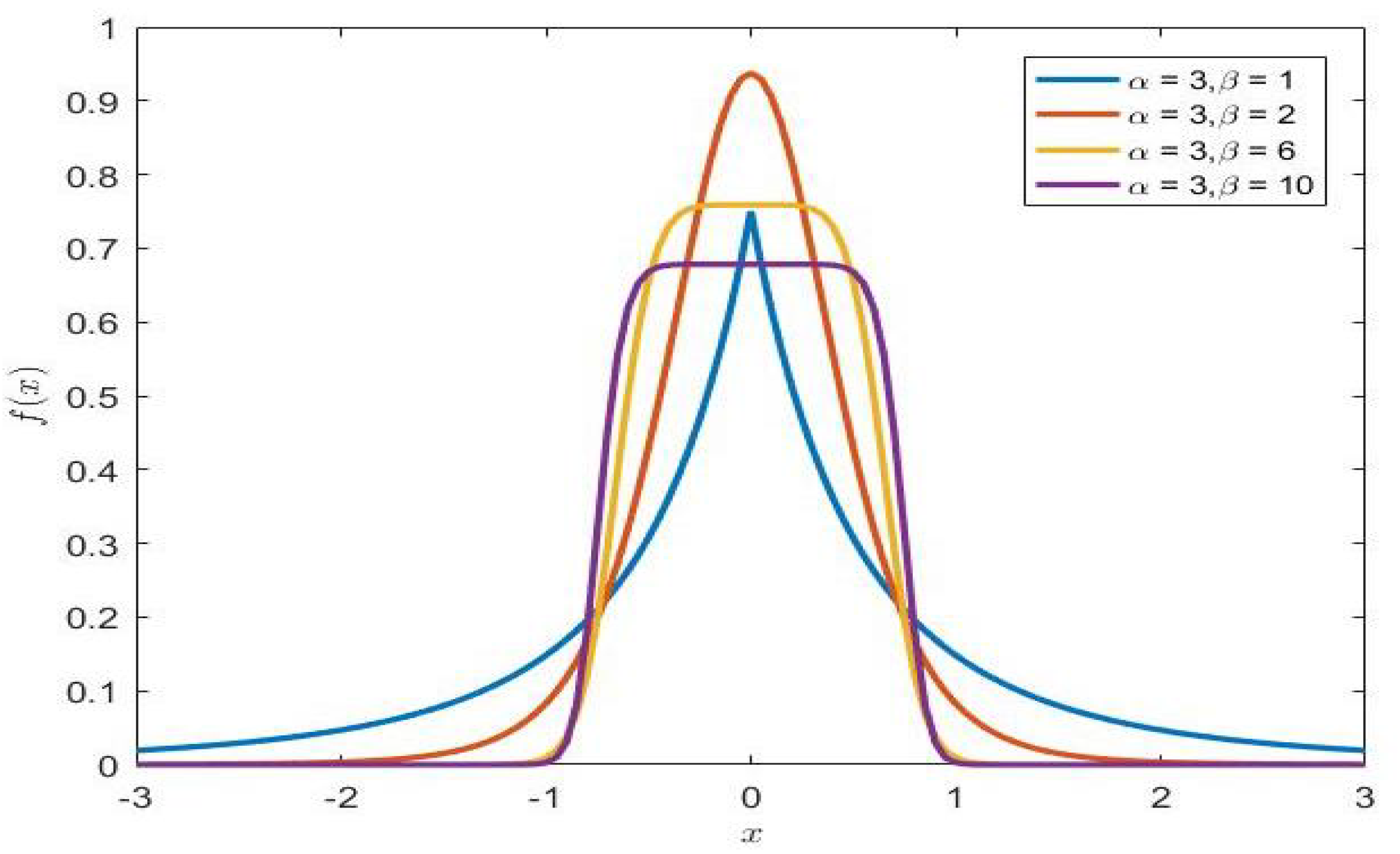
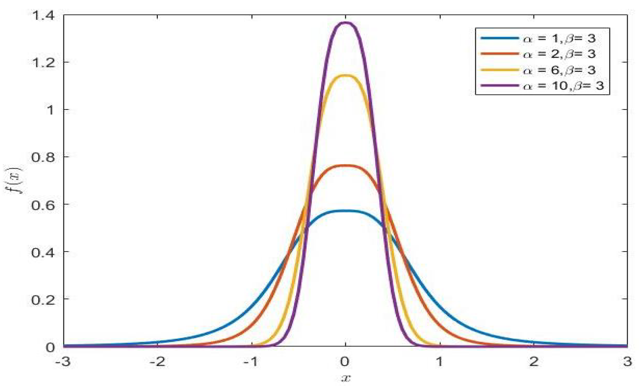
Theorem 1. The pdf of can be expressed as follows As is shown in the following two pictures (
Figure 1 and
Figure 2), two shape parameters (
and
) have a decisive effect on the shape of the density function. The density function has a heavier tail with a smaller value of
and
, but it is the opposite when the parameters
and
are larger. Furthermore, the shape parameter
plays a decisive role in the shape of the distribution and the change of parameter
can control the tail behavior.
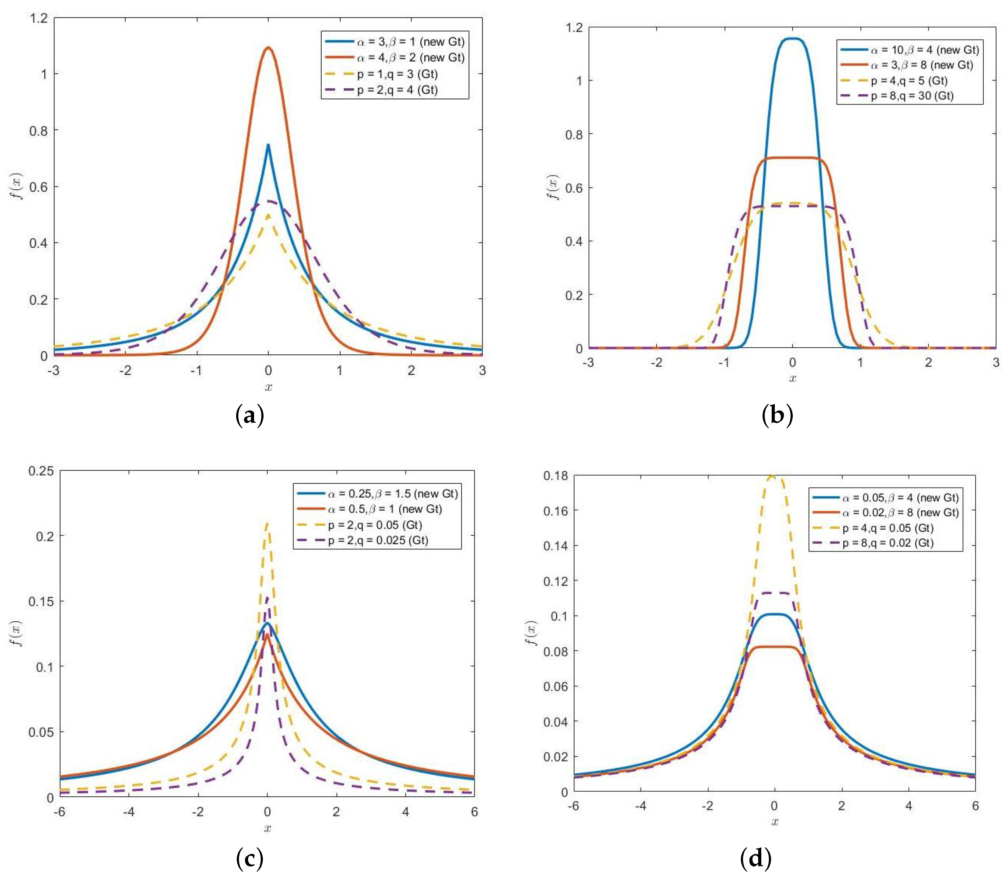
Figure 3 and
Figure 4 vividly describe the feature that the new Gt distribution is more suitable for fitting both the data with high kurtosis and with heavier tail than the Gt distribution coined by McDonald and Newey (1988) [
1] under appropriate parameter range from two perspectives respectively.
It is well-known that the pdf with a steeper shape is suitable for fitting data with high kurtosis, while a pdf with a smoother shape can be used for fitting heavy-tailed data. Since these two distributions we compare are symmetric, we use the maximum value of the pdf to characterize the steepness of its shape. Let and denote the maximum value of the pdf of Gt distribution and new Gt distribution, respectively.
Since the value of
has little effect on the value of
and
, we may assume that
. On the one hand, it is not very difficult to prove that, for a fixed
,
decreases monotonically with respect to
. Then we have:
. For
, the interval of the shape parameters
are (1, 10) and (0.1, 50), respectively. The reason for choosing these two ranges is that they include possible values for parameters in practical applications. From
Figure 3, we can obviously find that the range of function
is never greater than 1. This means that we can only adjust the parameter
to make the pdf of the Gt distribution have a steeper shape. On the other hand, for fixed
and
p, when
, both
and
tend to 0 but
has a faster convergence. This means that the pdf of the new Gt distribution proposed by us has a heavier tail when the parameters are within a reasonable range. Thus, the conclusion stated in the preceding paragraph is therefore self-evident.
The pdf generated under different shape parameters can be divided into four categories according to different shapes and the tail behavior, i.e., steep in shape and with a light tail, flat in shape and with a light tail, steep in shape and with a heavy tail, flat in shape and with a heavy tail. As is depicted in
Figure 4, the solid line denotes the new Gt distribution, and the dashed line represents the previous Gt distribution defined by McDonald and Newey (1988) [
1]. The subfigure
Figure 4a–d depicts the pdf of the Gt distribution and the new Gt distribution under the above four categories with different shape parameters, respectively. It can be seen from the figure that, if the parameter value is in a reasonable range, the shape of the new Gt distribution is more flexible and more suitable for fitting a wider range of data.
Some important properties of the new Gt distribution are stated as follows:
Proposition 1. If , and , then . .
Proposition 2. If and , then . .
Proposition 3. If , let and , then , where W is a random variable that only takes and satisfies .
From the above proposition, we can follow the following steps to generate random samples from :
- 1.
Generate and set .
- 2.
Generate .
if , set .
else set .
- 3.
Set and return Y.
Proposition 4. If , we have
the -th order moment of T is given byand the above equation exists for . Furthermore, from the symmetry of the distribution, we can conclude that , the kurtosis coefficient of T is given by the mean deviation of T is given by the shannon entropy is given by the Rényi entropy is given bywhere denote the digamma function.
3. Moments of Order Statistics
In this section, we derive the explicit expression for moments of order statistics from this distribution under the independent identically-distributed (IID) case and independent not identically-distributed (INID) case when the shape parameters and are both real non-integer or is an integer.
It is well-known that order statistics has always been a significant field in statistical research, especially in the study of distribution theory. In addition, it is necessary to study the related properties of order statistics, since many classical parameter estimation methods are based on the application of order statistics.
3.1. The IID Case
In this subsection, we obtain explicit expression for moments of order statistics from under IID case based on distribution transformation approach and recurrence relations when the shape parameter is either an integer or a real non-integer.
3.1.1. Shape Parameter Integer Case
Govindarajulu (1963) [
16] pointed out that the
k-th order moment of order statistics from a symmetric distribution can be linearly expressed by the moments of the order statistics from the corresponding folded distribution
where
denotes the
k-th moments of order statistics from symmetric distribution, while
denotes the
k-th moments of order statistics from the corresponding folded distribution.
Without loss of generality, let
. Making transformation
, we can derive the pdf of the random variable
Z as follows
Under the above transformation, the recurrence relations introduced by Govindarajulu (1963) [
16] becomes
Lemma 1. where denotes the k-th moments of order statistics from and denotes the k-th moments of order statistics from the corresponding folded distribution . Let
denote
, then
. The cdf of the random variable
Z can be written as
by binomial expansion we have
where
.
Let
denote the coefficient in the expansion of
. Obviously, the coefficients of this polynomial satisfy the following recursive relation
and with the following constraints
we can cauculate every coefficient striaghtly. Then
can be expressed as
It is noted that Equations (5) and (6) have similar forms, so the distribution
is said to have a minimum domains of attraction. With this conclusion,
is derived first. Through the traditional way, we obtain
and the above expression exists for
.
After that, using the well-known recurrence relations from David and Nagaraja (2003) [
17] presented below
where
and
We acquire the k-th order moment of order statistics from the distribution . When the sample size is n, the method of obtaining all the k-th moments of order statistics from when is an integer can be briefly described as follows
- 1.
Derive () by using the above approach.
- 2.
For
, derive
by using the recurrence relations in Equation (
4).
- 3.
By using the symmetry of Gt distribution, the k-th moments of the remaining order statistics can be calculated through .
Since this method makes full use of the characteristics of the distribution function and recursive relations, it is very efficient and can avoid a lot of unnecessary calculations.
3.1.2. Shape Parameter or Non-Integer Case
The generalized Kampe de Feriet function from Exton (1978) [
18] is defined by
where
,
for
,
,
, or
and
,
.
By using the above special function, we derive the following theorem:
Theorem 2. If the shape parameter α is a real non-integer, the k-th order moment of order statistics from can be calculated by the following convergent expressionwhere Theorem 3. If the shape parameter is a real non-integer, in Theorem 2 can be calculated by 3.2. The INID Case
Suppose that
are independent but not identical random samples from the following pdf with the same shape parameter
but the rest of the parameters are different
Theorem 4. If the shape parameter is a real non-integer, the m-th order moment of order statistics from can be calculated by the following convergent expressionwhere 4. Product Moments and Variance–Covariance Matrix of Order Statistics
In this section, we obtain explicit expressions for product moments and the corresponding variance–covariance matrix of order statistics from this distribution based on recurrence relations and distribution transformation when the shape parameter is an integer.
The covariance matrix of order statistics plays a big role in a number of estimation methods based on order statistics, such as the least square estimation and the BLUE for location-scale parameters. In addition, obtaining a covariance matrix of order statistics is usually not an easy task and requires some related skills.
Under transformation
introduced in the previous section, the recursive relations for the product moment of order statistics from a symmetric distribution between its corresponding folded distribution becomes
The cdf of the random variable Z is denoted by and suppose , then let denote . Obsiviously, we can write that .
First of all, we decide to derive
. Taking the well-known expression of the product moment of order statistics and then using the binomial expansion, we obtain
where
After that, we attempt to derive the double integral
. By the multinomial theorem we have
We denote the inner integral
of the above double integral
by
and it can be calculated as follows
Notice that
is still a positive integer, then expanding the integrand on the right hand side of the above expression in terms of
, we acquire
Using the fact that
by putting Equations (11) and (12) into
, we obtain
The above equation will exists for
. Finally, using recurrence relations from Arnold et al. (2008) [
19]:
For any arbitray distribution and
we can derive a closed-form expression for every product moment and the corresponding variance–covariance matrix of order statistics from
.
When the sample size is n, the method of obtaining all the product moments and variance–covariance matrix for order statistics from can be briefly described as:
- 1.
Derive () by using the above approach.
- 2.
For
, obtain
by using recurrence relations in Equation (
9) and obtain the covariance
by
.
- 3.
By using the symmetry of Gt distribution and the variance–covariance matrix, the remaining covariance of order statistics can be calculated by and .
5. Parameter Estimation
In this section, we propose several parameter estimation methods for the new Gt distribution.
5.1. Modfied Method of Moments
In this subsection, a modified method of moments (MMOM) for the parameters of is proposed.
Let
be a random sample from
. Making transformation
, the
k-th theoretical central moments of
Y are given by
The MMEs of the new distribution after transformation can be obtained by equating the first three theoretical central moments of
Y with the corresponding central sample moments. Eliminating the scale parameter
, we acquire
In order to establish an effective algorithm to obtain the numerical solution of the above equations, we propose the following theorem:
Theorem 5. Letthen we assert that is a monotonically-decreasing function of the parameters α and β. In addition, the function has the following limiting properties With the above theorem, the steps of the algorithm are presented by the following forms
- 1.
Assign an initial values
, and then substitute
into Equation (
15). Since
is monotonically-decreasing with respect to parameter
,
in the
R function can be used to derive
.
- 2.
Substitute
into Equation (
16), since
is monotonically-decreasing with respect to parameter
, using
in
R function then we obtain
.
- 3.
If the norm of vector exceed the prescribed value , then 2–3 are repeated. Otherwise, the iteration is broken up and the values generated in the last iteration are determined to be estimates of the shape parameters and .
5.2. MLE Using the EM Algorithm
In this subsection, an EM-type algorithm to determine the MLEs for the parameters of is established.
Through the method of distribution construction, the pdf of the new Gt distribution is treated as a marginal pdf of a bivariate distribution and this bivariate distribution function can be expressed as the product of two common distributions. After that, we treat one random variable in the bivariate distribution as an observed variable, while the other as an unobserved variable, so that the EM algorithm can be applied to obtain the MLE. At the same time, this idea is also widely used to derive the MLE of other distributions. See [
15,
20,
21] for more details about recent works in this topic.
First proposed by Dempster (1977) [
22], the EM algorithm is a powerful tool to deal with estimation problem under missing data situation. In this subsection, we are going to use the EM algorithm to acquire the MLEs of
based on Proposition 2. Let
denote the observed data,
on behalf of the unobserved data. Combining
Y and
U together we derive the complete data denoted by
. Besides that, let
represent the vector of parameters. Invoking Proposition 2, the complete log-likelihood function can be expressed as follows
It is well-known that the EM framework is an iterative algorithm consisting of two steps; namely, the expectation step (E-step) and the maximization step (M-step).
E-step: Given the observed data set
and parameter estimation values
for the
h-th iteration, the conditional expectation of the complete log-likelihood function can be calculated as follows
where
In the EM algorithm, the M-step needs to maximize the conditional expectation obtained by E-step and the suggested framework can be briefly described as follows
- 1.
Update
through the following nonlinear equation and the corresponding numerical procedures is recommended for
in
R program.
- 2.
Update
through the following explicit expression
- 3.
Update
by maximizing the observed data log-likelihood function
For the initial values , we recommend conducting numerical procedures such as in R program for maximizing the corresponding likelihood function or using the estimation values from the method of moments.
5.3. Explicit Expressions for Asymptotic Variances and Covariances of the Estimates under the EM Algorithm
In this subsection, we obtain closed-form expression for the asymptotic variances and covariances of the estimates under the EM algorithm. Louis (1982) [
23] coined the missing information principle to acquire an information matrix in a situation containing latent variables. This principle is given by
In the following paper, we will denote the complete, observed and missing information by
,
and
, respectively. Then the observed information
is calculated by:
5.3.1. Complete Information Matrix
Taking the second-order partial derivatives of the complete log-likelihood function in Equation (
17) and applying the definition of the fisher information, then after some calculation, we obtain
where
The second-order partial derivatives of the complete likelihood function and the calculation method of the complete information are shown in the
Appendix A.3 (Part III).
5.3.2. Missing Information Matrix
From Proposition 2, the logarithm of the joint density function of latent variable
U given
Y can be written as
After taking the second-order partial derivatives with respect to
,
and
, and utilizing the results in
Section 5.2, the elements of the missing information matrix
are presented as follows
5.4. MLE via a New Iterative Algorithm
In this subsection, we propose a new iterative algorithm to obtain the MLEs for the parameters of because of the difficulty of sloving the estimation equations directly.
Let
be a random sample from
, and the log-likelihood function is given by
With partial derivatives respect to
, we obtain
Instead of sloving all three preceding equations simultaneously, we propose a new algorithm because of the complexity of the third equation of Equation (
18). In order to establish the new approach, the following lemma is necessary
Lemma 2. For any fixed β, the following equationsalways possess a convergent solution of parameter and is independent of the initial values . Moreover, the algorithm for obtaining the solution of the equation in Lemma 2 is shown below
- 1.
Given arbitrary initial values and .
- 2.
Substitute
into the first equation of Equation (
19), and we obtain
.
- 3.
Substitute
into the second equation of Equation (
19), and we obtain
.
- 4.
If the norm of vector exceed the prescribed value , then 2–3 are repeated. Otherwise, the iteration is broken up and the values generated in the last iteration are determined to be solution of this equation.
In what follows, the new algorithm to acquire the solution of Equation (
18) can be briefly described as
- 1.
Give an appropriate interval for the shape parameter , and then generate a set of values of this parameter at an appropriate distance within the interval and represent the j-th element of this vector by .
- 2.
Assigning
into the first two equations of Equation (
18)and applying Lemma 2, we can obtain their convergence solution denoted by
.
- 3.
Repeat this procedure and observe the sign-changing in the left-hand side of the third equation of Equation (
18). Then, by interpolating on
values, we derive the final estimate
, which makes the third equation equals to 0 or sufficiently close to 0. Finally, by substituting
into the first two equations of Equation (
18), we derive the final estimates denoted by
.
It is noteworthy that this algorithm is applicable when the sample kurtosis is greater than 2.7. Comparing with other numerical methods, our new algorithm requires less precision of initial values and can obtain convergent solutions.
5.5. An Improved PWM Estimation
In this subsection, we propose an improved PWM (IPWM) estimation based on order statistics transformation for and develop the corresponding algorithm to implement this novel method.
PWM estimation is a very effective and commonly used method for parameter estimation of distributions with heavy tails. Among many parameter estimation methods proposed so far, PWM and MLE are the two most commonly-used methods that have similar priority.
Let
be a random sample from
and
behalf of the corresponding order statistics. The traditional theoretical PWM was introduced by Greenwood et al. [
24] as an alternative to the method of moments given in the following equation
Taking
, the moments become
denoted by
. Wang (1990) [
25] obtained an unbiased estimator of
through linear combination of order statistics as follows
However, applying the traditional PWM directly can cause many problems due to the complexity of the distribution function. For example, intricacy expressions of the theoretical PWM will make the estimation equation tedious and difficult to be numerically optimized, thus impeding the use of this estimation method. As a result, we decide to make isotone transformation
. After this monotone transformation, the estimation equation becomes simple and easy to solve by a numerical approach. The improved theoretical PWM (denoted by
) under this transformation is given by
The corresponding improved sample PWM (denoted by
) is defined as follows
where
and
is an initial guess of the scale parameter
.
From Equation (
20), we can derive the 2–5th improved theoretical PWM as follows
According to the traditional idea of the method of moments, let the improved theoretical PWM
equal to the corresponding improved sample PWM. Then we can obtain an equation set whose solution is the estimation of the unknown parameters. Due to the complexity of these equations, we transform the search for the solution of this equation set into an optimization problem and acquire the simultaneous estimation of the shape parameters denoted by
through minimizing the following expression to avoid failures during optimization
Numerical techniques are recommended, such as the function in R program and the method will be chosen for .
Finally, the estimation of the scale parameter
can be obtained through the first original sample PWM of the random variable
X with analytical expression given by the following equation
In the study, we found that the estimation results are sensitive to the choice of the initial guess . Therefore, we introduce the following two methods to discuss the choice of this parameter.
Method 1 (A two step estimation method)
- 1.
Take a consistent estimate of parameter as the initial guess of it, such as MLE.
- 2.
Substitute this estimate value
into Equation (
22) then we derive the improved PWM-estimation of the two shape parameters. The estimation for the scale paramter
can be obtained through Equation (
23).
Through this method, considering that it is relatively fixed to select the value of parameter , and the final estimations are largely dependent on this parameter, sometimes it is inevitable that the fixed parameter does not apply to all samples. As a result, we establish the following algorithm, which can flexibly select the parameter and the suggested framework can be briefly described as:
Method 2 (A selection algorithm)
- 1.
Give an appropriate interval for the parameter , generate a set of at appropriate distance within the interval and represent the h-th element of the vector by .
- 2.
Substitute each
into Equation (
22) to acquire simultaneously estimation for two shape parameters denoted by
and
. After that, cauculate the corresponding original 6th theroetical PWM-kuritosis through the following equation
- 3.
Repeate 2 and cauculate ( and denote the original 6th and 2th sample PWM of the random variable X, respectively). Then, interpolate on values and derive that minimize .
- 4.
Substituting
into Equation (
22) we derive the final estimation for two shape parameters and final estimation for
can be obtained form Equation (
23).
5.6. Parameter Estimation of
In this subsection, we propose a profile maximum likelihood approach (PLA) using the EM algorithm to cope with parameter estimation for the new Gt distribution with four parameters.
In fitting problems with the distribution of data with better symmetry, three factors are usually comprehensively scrutinized, namely location information, scale parameters, and shape parameters. Therefore, with the addition of the location parameter, we focus on parameter estimation problem of .
Balakrishnan (2019) [
20] applied this approach to determine the MLEs for the parameters of Student’s
t Birnbaum-Saunders distribution. As Balakrishnan points out, this method is an example of an exhaustive search. Due to the addition of location parameter
, the estimation equation becomes very complicated. To overcome this difficulty,
can be assumed as a natural number through profile likelihood approach, reducing the dimension of the problem with four parameters to that with three. Then the EM algorithm for the three-parameter case described in the preceding chapter comes in handy here.
Let
be a random sample from
. In this case, the log-likelihood function is given by
Since , we can assert that the likelihood function is bounded when the parameter are fixed.
A suggested framework for the PLA using the EM algorithm is briefly described as follows:
- 1.
Give an appropriate interval for the location parameter . Then generate a set of at appropriate distance within the interval and represent the j-th element of the vector by .
- 2.
Substitute each in the log-likelihood function and implement the EM algorithm to derive the MLEs of .
- 3.
Repeating this procedure, and then interpolating on values, we obtain a curve of values of the log-likelihood function and choose the value of that maximizes the curve as .
- 4.
Substitute in the log-likelihood function and implement the EM algorithm to determine the final MLEs denoted by .
The implementation for the EM algorithm is similar to
Section 5.2, just replace all the
in the partial derivative of
and the integral with
. The trace of the log-likelihood function is depicted in
Figure 5. Through simulation research, we find that this algorithm performs well for
and is more accurate and stable than using the sample mean as the estimation of the location parameter
directly under a small sample size.
6. Simulation Study
In this section, we conduct a simulation study to illustrate the performance of the proposed estimation methods and compare these simulation results under different parameter values and different sample sizes.
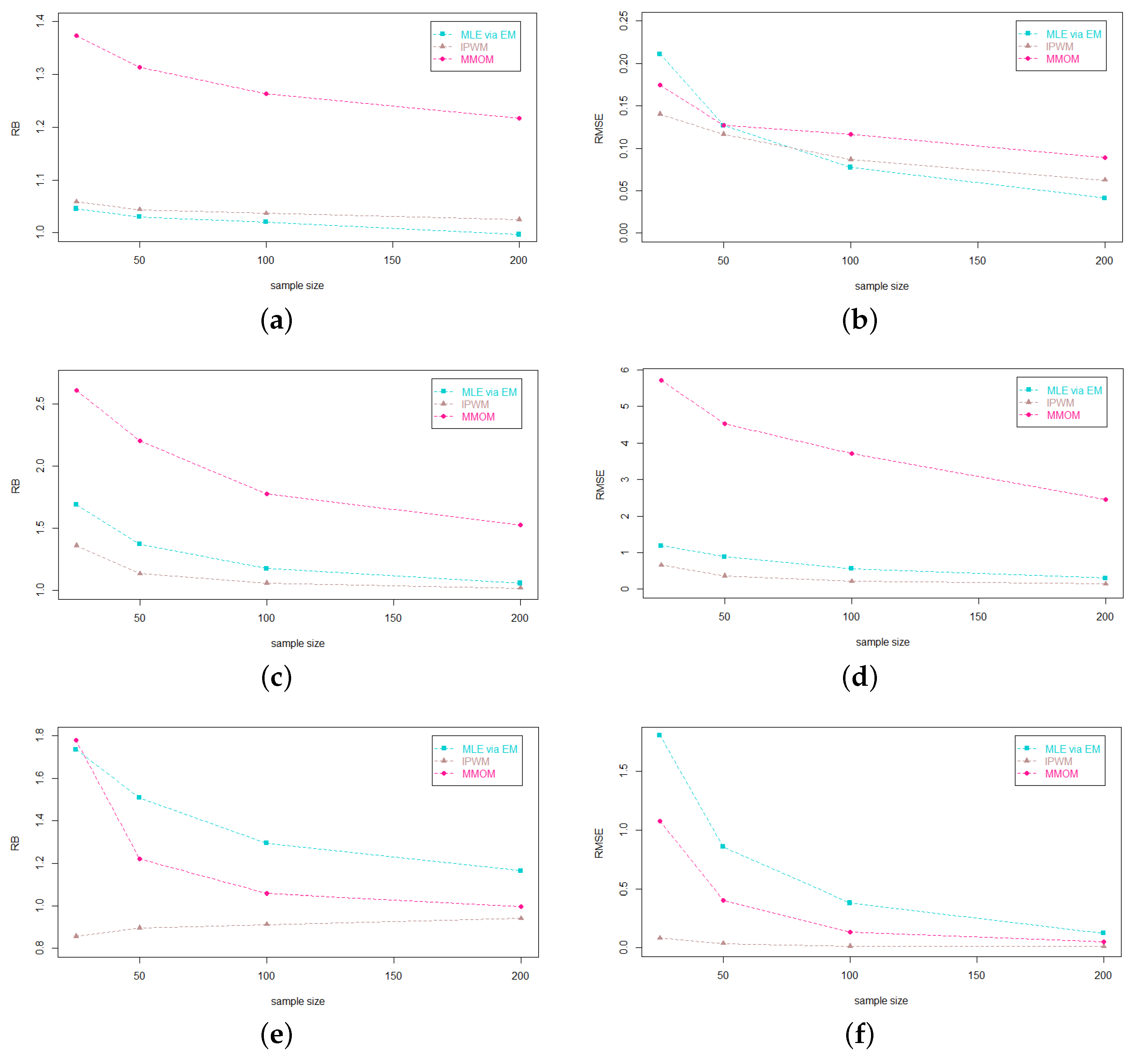
According to the actual demand, the sample size will be chosen for 25, 50, 100 and 200. We perform Monte Carlo simulations and evaluate the performance of the considered methods through relative bias (RB) and relative mean-square errors (RMSE). These two indicators will be computed with 5000 replications at the same time and they are defined as follows
This section will be detailed in three parts. First of all, we conduct a comparative study for three different estimation methods (MMOM, MLE using the EM algorithm and IPWM) of
. We mainly study the influence of shape parameter
on the performance of these methods. As a result, we fix
,
, and
will be chosen for
, respectively. To show the comparison more vividly, we draw the following pictures (
Figure 6,
Figure 7 and
Figure 8) and the estimated values of these three parameters are shown in
Appendix A.4 (Part IV).
It can be seen that the two indicators RB and RMSE of these three estimation methods gradually decrease with the increase of sample size. As the value of the shape parameter, , increases, the estimation accuracy of the IPWM and the MLE using the EM algorithm for shape parameter gradually becomes better. Meanwhile, we can conclude that the IPWM performs best for both accuracy and stability, especially for the distribution has a heavier tail, while the MLE using the EM algorithm is the second on the whole. The performance of these two methods is comparable under a large sample size or high theoretical kurtosis. Furthermore, the IPWM is suitable for distributions with heavy tails and the MLE using the EM algorithm can become an alternative estimation method for steep-shaped distributions or under large sample size.
Second, a comparative study of the MLE using the EM algorithm and the MLE via a new iterative algorithm with sample kurtosis more than 2.7 is considered. The numerical results are presented in
Table 1 for fixed
,
,
,
.
Table 1 suggests that the new iterative algorithm performs better than the EM algorithm under sample kurtosis that exceeds 2.7 in general, especially for the estimation accuracy and stability of shape parameter
. For shape parameter
, the iterative algorithm provides higher estimation accuracy while the EM algorithm is more stable.
At last, a simulation study for the PLA using the EM algorithm for
(
) considered in
Section 5.6 will be performed. We mainly focus on the influence of shape parameter
and sample size on the estimation performance of this method. Therefore, we fix
and
will be chosen for
, respectively. Line graphs of the relationship between RB, RMSE and sample sizes with different value of shape parameter
were shown below (
Figure 9) and the estimated value for these parameters are given in
Table A4.
Figure 9 reveals that as the value of the shape parameter
increases, the estimation results become better and better. It is concluded that with the increase of the theoretical kurtosis, the accuracy and stability of the MLEs are gradually improved. In addition, the estimation effect of location parameter,
, and shape parameter,
, is less affected by the change of shape parameter
, while that two indicators for the scale parameter,
, and shape parameter,
, are more sensitive to the change of it. This means that it is not very difficult to estimate the location parameter for a distribution with good symmetry, while the shape parameters of a heavy tail distribution are more difficult to estimate.
7. Real Data Analysis
In this section, a real data analysis is performed to illustrate the feasibility of the new Gt distribution and a comparison with the Gt distribution is also presented.
These data concerned U.S. stock market and were introduced by Shen et al. (2020), [
26]. The basic description of the statistical characteristics of the data set are shown in
Table 2, which containing the sample size
n, the mean value
, the standard deviation
S, the asymmetry coefficient
, the kurtosis coefficient
, the minimum value min
, and the maximum value max
. It can be seen from the table that the data set has good symmetry and higher kurtosis.
To obtain the MLEs of the unknown parameters, the PLA depicted in
Figure 10 is recommended to avoid possible numerical optimization problems. The fitting results of these two distributions and the estimated parameter values are presented in
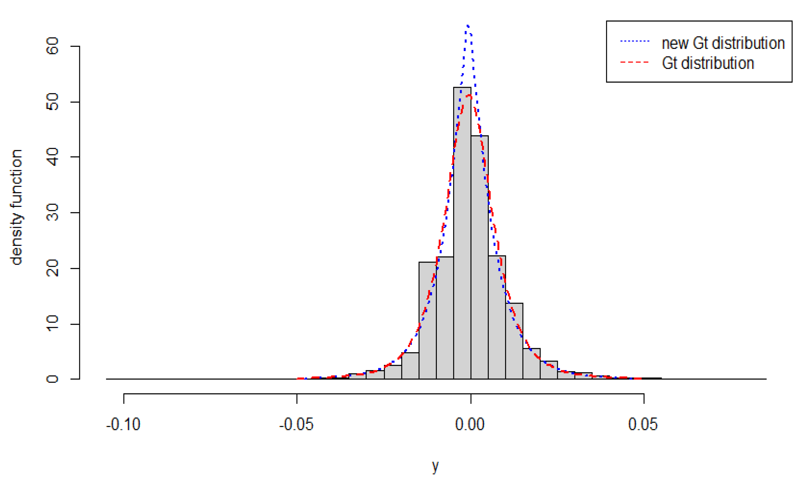
Table 3. Based on the AIC criterion, we can infer from it that the new Gt distribution is slightly more suitable for fitting this data set than the Gt distribution. The histogram of the considered data with the two density functions we fitted is drawn in
Figure 11. It is clearly seen that the pdf of the new Gt distribution is steeper in shape with a lighter tail, while the Gt distribution is the opposite.
8. Conclusions
In this paper, we coin a new Gt distribution that is suitable for fitting both the data with high kurtosis and a heavy tail based on a construction approach. Firstly, we have investigated the main properties of the new distribution including moments, skewness coefficients, kurtosis coefficients and random number generation. Secondly, we have derived the explicit expression for the moments of order statistics as well as its corresponding variance–covariance matrix through recurrence relations and the distribution transformation technique. The so obtained method has high efficiency and can greatly reduce the computation time. After that, we have focused on the parameter estimation of this new Gt distribution. Several estimation methods including MMOM, MLE using the EM algorithm, MLE using a new iterative algorithm and IPWM have been introduced. Among all these estimation methods, the IPWM performs best on the whole and this novel method makes the parameter estimation method of this distribution not limited to MLE and MMOM. Furthermore, the new iterative algorithm to acquire MLE is more suitable than the EM algorithm when the sample kurtosis is more than 2.7. For four-parameter new Gt distribution, we have established an EM-type algorithm through the profile maximum likelihood approach and discovered that the variation of the shape parameter has a significant effect on the estimation performance of scale parameter and shape parameter . However, there are still some limitations and areas to be improved in our research. The parameter estimation method is limited to PLA using the EM algorithm when the distribution has a heavier tail. Therefore, proposing more efficient and accurate estimation methods will be the focus of our future research. Besides, the new Gt distribution is suitable for fitting data with good symmetry. In future work, it can be applied for the asymmetric situation by adding a skew parameter.
Author Contributions
R.G.: Conceptualization, Formal analysis, Methodology, Software, Writing—original draft, Data curation; W.C.: Conceptualization, Formal analysis, Methodology, Investigation, Supervision, Funding acquisition, Writing—review and editing; X.Z.: Methodology, Formal analysis, Supervision, Writing—review and editing, Data curation, Funding acquisition, Validation; Y.R.: Funding acquisition, Writing—review and editing. All authors have read and agreed to the published version of the manuscript.
Funding
This research was partially supported by the National Natural Science Foundation of China (Grant No. 11701021), the National Natural Science Foundation of China (Grant No. 11801019), the Beijing Natural Science Foundation (Grant No. Z190021), the Science and Technology Program of Beijing Education Commission (Grant No. KM202110005013) and the Science and Technology Project of Beijing Municipal Education Commission(Grant No. KM202110005012).
Institutional Review Board Statement
Not applicable.
Informed Consent Statement
Not applicable.
Data Availability Statement
Data available in a publicly accessible repository; the data presented in this study are openly available in Shen et al., (2020).
Conflicts of Interest
The authors declare no conflict of interest.
Appendix A
Appendix A.1. Part I
Proof. Proof of Theorem 1
According to the pdf of the quotient of two random variables, we have
Let
, we obtain
by substituting the above expression into (A1) we can derive the pdf of the random variable
T in Theorem 1. □
Proof. Proof of Proposition 1
Appendix A.2. Part II
Proof. Proof of Lemma 1
Notice that
the follwing steps are similar to Govindarajulu (1963) [
16]. □
Proof. Proof of Theorem 2
Through the traditional way for cauculating the
k-th moments of order statistics, we have
From the symetric properties of this distribution, let
, we have
We notice that
where
denote the incomplete beta function. -4.6cm0cm
When
is a real non-integer, by using generalized multinomial theorem, we obtain
With the above equations
can be rewritten as
and the above expression exists for
.
For a suifficent large
N, we can bound that
□
Proof. Proof of Theorem 3
By using the genralized multinomial theorem, we acquire
and
By substituting the above two expressions into
, we obtain
this expression exists for
. □
Proof. Proof of Theorem 4
Let
denote the cdf with parameters
. Barakat and Abdelkader (2004) [
27] proposed the following expression to cauculate the moments of order statistics for the INID case
where
Let
, from the symetric properties of this distribution we can reexpress
as
From
Section 2 we know that
. Using series expansion, we immediately acquire the expressions as follows
By subsituting the above equation into the expression of
, we obtain
By using the defination of the generalized Kampe de Feriet function, the above equations can be reexpressed as
and the above expression exists for
. □
Appendix A.3. Part III
Proof. Proof of Theorem 5
In order to prove the monotony, we take the logarithms of the above two functions, respectively. Differentiating with respect to parameter
, we obtain
as a result
is monotonically decreasing with respect to the parameter
.
For
, taking logarithm, we have
Taking partial derivative with respect to parameter
, we have
Taking partial derivative with respect to parameter
, we obtain
Besides that, it is easy to prove that
With the above conclusions, the result of the theorem is obvious. □
Cauculation for the asymptotic variances and covariances of the estimates under EM algorithm
The second partial derivatives of the complete likelihood function is given by
From Proposition 2, let
, the joint density function of
is given by
then through the above density function, the expectation can be calculated as
The inner integral can be calculated as
By substituting the above expression into the double integral, we have
On the same way, we obtain
Proof. Proof of Lemma 2
First of all, we decide to prove that the first and the second equation always has a unique solution for fixed and , respectively.
Let .
Obviously, this function is monotonically increasing with respect to and , . Therefore, there must exist a root for in .
On the same way, let and it is easy to prove that this function is monotonically decreasing with respect to .
From Taylor’s theorem we obtain
obviously, for fixed
and
,
and
. Therefore, there must exist a root for
in
.
After that, we decide to prove the convergence of the iterative algorithm. Assuming that denote the solution of the equations and represent the values of p-th iteration, we have
Case I. The proof is conducted by mathematical induction, for , the conclusion clearly holds.
Assume that for
, we have:
, then
and
are obtained from the following two equations, respectively
Obviously, we can conclude that
and this is equivalent to
.
and
are obtained from the following two equations, respectively
and this is equivalent to
.
Since the two squences statisfy: , , the conclusion holds.
Case II. The proof in this case is similar to the above case. □
In a word, this conclusion can be summarized as follows:
- 1.
if , the sequence are both monotonically increasing and converge from the left side to the solution,
- 2.
if , the sequence are both monotonically decreasing and converge from the right side to the solution.
Appendix A.4. Part IV
Table A1.
Estimation value under , , .
Table A1.
Estimation value under , , .
| Method | Sample Size | | | |
|---|
| | n = 25 | 1.584 | 7.83 | 2.314 |
| | n = 50 | 1.528 | 6.615 | 2.147 |
| MMOM | n = 100 | 1.463 | 5.331 | 2.105 |
| | n = 200 | 1.265 | 4.584 | 2.071 |
| | n = 25 | 1.18 | 5.174 | 3.228 |
| | n = 50 | 1.132 | 4.421 | 2.482 |
| MLE via EM | n = 100 | 1.104 | 3.814 | 2.364 |
| | n = 200 | 1.036 | 3.341 | 2.201 |
| | n = 25 | 1.109 | 3.659 | 3.766 |
| | n = 50 | 1.062 | 3.49 | 2.882 |
| IPWM | n = 100 | 1.033 | 3.3885 | 2.528 |
| | n = 200 | 1.022 | 3.308 | 2.35 |
Table A2.
Estimation value under , , .
Table A2.
Estimation value under , , .
| Method | Sample Size | | | |
|---|
| | n = 25 | 1.373 | 7.830 | 5.339 |
| | n = 50 | 1.314 | 6.615 | 3.659 |
| MMOM | n = 100 | 1.263 | 5.331 | 3.176 |
| | n = 200 | 1.217 | 4.584 | 2.98 |
| | n = 25 | 1.046 | 5.073 | 5.207 |
| | n = 50 | 1.032 | 4.119 | 4.524 |
| MLE via EM | n = 100 | 1.021 | 3.531 | 3.884 |
| | n = 200 | 0.997 | 3.181 | 3.481 |
| | n = 25 | 1.059 | 4.087 | 2.569 |
| | n = 50 | 1.044 | 3.408 | 2.691 |
| IPWM | n = 100 | 1.037 | 3.182 | 2.737 |
| | n = 200 | 1.025 | 3.05 | 2.825 |
Table A3.
Estimation value under , , .
Table A3.
Estimation value under , , .
| Method | Sample Size | | | |
|---|
| | n = 25 | 1.298 | 5.403 | 6.281 |
| | n = 50 | 1.267 | 4.933 | 5.124 |
| MMOM | n = 100 | 1.231 | 4.508 | 4.619 |
| | n = 200 | 1.197 | 3.718 | 4.358 |
| | n = 25 | 1.067 | 5.214 | 7.179 |
| | n = 50 | 1.022 | 4.155 | 5.794 |
| MLE via EM | n = 100 | 1.002 | 3.513 | 5.039 |
| | n = 200 | 0.999 | 3.115 | 4.402 |
| | n = 25 | 0.887 | 4.056 | 3.672 |
| | n = 50 | 0.919 | 3.224 | 3.496 |
| IPWM | n = 100 | 0.932 | 3.075 | 3.318 |
| | n = 200 | 0.954 | 2.976 | 3.132 |
Table A4.
Estimation value for PLA using the EM algorithm under different (fixed , , ).
Table A4.
Estimation value for PLA using the EM algorithm under different (fixed , , ).
| Value of | Sample Size | | | | |
|---|
| | n = 25 | 1.0082 | 1.4411 | 4.3878 | 4.8281 |
| | n = 50 | 0.9986 | 1.3755 | 3.7841 | 3.3574 |
| n = 100 | 0.9997 | 1.2325 | 3.0712 | 2.6304 |
| | n = 200 | 0.9999 | 1.1233 | 2.5676 | 2.2731 |
| | n = 25 | 1.0036 | 1.3598 | 4.9423 | 4.6686 |
| | n = 50 | 1.0029 | 1.2715 | 4.0851 | 3.4920 |
| n = 100 | 0.9994 | 1.1692 | 3.4725 | 2.6501 |
| | n = 200 | 1.0006 | 1.0876 | 2.962 | 2.3084 |
| | n = 25 | 0.9741 | 1.2494 | 5.0373 | 4.6552 |
| | n = 50 | 0.9896 | 1.1827 | 4.3119 | 3.4574 |
| n = 100 | 1.0005 | 1.1058 | 3.7419 | 2.6380 |
| | n = 200 | 0.954 | 1.0006 | 3.3182 | 2.2532 |
References
- McDonald, J.B.; Newey, W.K. Partially Adaptive Estimation of Regression Models via the Generalized t Distribution. Econom. Theory 1988, 4, 428–457. [Google Scholar] [CrossRef]
- Nadarajah, H.N. On the Generalized t (Gt) Distribution. Statistics 2008, 42, 467–473. [Google Scholar] [CrossRef]
- Galbraith, J.W.; Zhu, D. A Generalized Asymmetric Student-t Distribution with Application to Financial Econometrics. J. Econom. 2010, 157, 297–305. [Google Scholar] [CrossRef][Green Version]
- Harvey, A.; Lange, R.J. Volatility Modeling with a Generalized t Distribution. J. Time Ser. Anal. 2017, 38, 175–190. [Google Scholar] [CrossRef]
- Peel, D.; McLachlan, G.J. Robust Mixture Modelling Using the t Distribution. Stat. Comput. 2000, 10, 339–348. [Google Scholar] [CrossRef]
- Arslan, O.; Genç, A.İ. Robust Location and Scale Estimation Based on the Univariate Generalized t (GT) Distribution. Commun.-Stat.-Theory Methods 2003, 32, 1505–1525. [Google Scholar] [CrossRef]
- Paula, G.A.; Leiva, V.; Barros, M.; Liu, S. Robust Statistical Modeling Using the Birnbaum Saunders t Distribution Applied to Insurance. Appl. Stoch. Model. Bus. Ind. 2012, 150, 169–185. [Google Scholar] [CrossRef]
- Çankaya, M.N.; Arslan, O. On the Robustness Properties for Maximum Likelihood Estimators of Parameters in Exponential Power and Generalized t Distributions. Commun.-Stat.-Theory Methods 2018, 49, 607–630. [Google Scholar] [CrossRef]
- Arslan, O.; Genç, A.İ. The Skew Generalized t Distribution as the Scale Mixture of a Skew Exponential Power Distribution and Its Applications in Robust Estimation. Statistics 2009, 43, 481–498. [Google Scholar] [CrossRef]
- Venegas, O.; Rodríguez, F.; Gómez, H.W.; Olivares-Pacheco, J.F.; Bolfarine, H. Robust Modeling Using the Generalized Epsilon Skew t Distribution. J. Appl. Stat. 2012, 39, 2685–2698. [Google Scholar] [CrossRef]
- Papastathopoulos, I.; Tawn, J.A. A Generalised Student’s t-Distribution Stat. Probab. Lett. 2013, 83, 70–77. [Google Scholar] [CrossRef]
- Acitas, S.; Senoglu, B.; Arslan, O. Alpha-Skew Generalized t Distribution. Rev. Colomb. Estad. 2015, 38, 371–384. [Google Scholar] [CrossRef]
- Lak, F.; Alizadeh, M.; Monfared, M.E.D.; Esmaeili, H. The Alpha-Beta Skew Generalized t Distribution: Properties and Applications. Pak. J. Stat. Oper. Res. 2019, 46, 605–616. [Google Scholar] [CrossRef]
- Genç, A.İ. The Generalized T Birnbaum-Saunders Family. Statistics 2013, 47, 613–625. [Google Scholar] [CrossRef]
- Balakrishnan, N.; Kundu, D. Birnbaum-Saunders Distribution: A Review of Models, Analysis, and Applications. Appl. Stoch. Model. Bus. Ind. 2019, 35, 4–49. [Google Scholar] [CrossRef]
- Govindarajulu, Z. Relationships Among Moments of Order Statistics in Samples from Two Related Populations. Technometrics 1963, 5, 514–518. [Google Scholar] [CrossRef]
- David, H.A.; Nagaraja, H.N. Order Statistics, 3rd ed.; John Wiley & Sons, Inc.: Hoboken, NJ, USA, 2003. [Google Scholar]
- Exton, H. Handbook of Hypergeometric Integrals: Theory, Applications, Tables, Computer Programs; Ellis Horwood: Chichester, UK, 1978. [Google Scholar]
- Arnold, B.C.; Balakrishnan, N.; Nagaraja, H.N. A First Course in Order Statistics; John Wiley & Sons, Inc.: Hoboken, NJ, USA, 2008. [Google Scholar]
- Balakrishnan, N.; Alam, F.M.A. Maximum Likelihood Estimation of the Parameters of Student’s t Birnbaum-Saunders Distribution: A Comparative Study. Commun.-Stat.-Simul. Comput. 2019, 2, 1–30. [Google Scholar] [CrossRef]
- Poursadeghfard, T.; Jamalizadeh, A.; Nematollahi, A. On the Extended Birnbaum—Saunders Distribution Based on the Skew-t-Normal Distribution. Iran. J. Sci. Technol. Trans. Sci. 2019, 43, 1689–1703. [Google Scholar] [CrossRef]
- Dempster, A.P. Maximum Likelihood from Incomplete Data via the EM Algorithm. J. R. Stat. Soc. 1977, 39, 1–38. [Google Scholar]
- Louis, T.A. Finding the Observed Information Matrix When Using the EM Algorithm. J. R. Stat. Soc. Ser. Stat. Methodol. 1982, 44, 226–233. [Google Scholar]
- Greenwood, J.A.; Landwehr, J.M.; Matalas, N.C.; Wallis, J.R. Probability Weighted Moments: Definition and Relation to Parameters of Several Distributions Expressable in Inverse Form. Water Resour. Res. 1979, 15, 1049–1054. [Google Scholar] [CrossRef]
- Wang, Q.J. Estimation of the GEV Distribution from Censored Samples by Method of Partial Probability Weighted Moments. J. Hydrol. 1990, 120, 103–114. [Google Scholar] [CrossRef]
- Shen, Z.; Chen, Y.; Shi, R. Modeling Tail Index with Autoregressive Conditional Pareto Model. J. Bus. Econ. Stat. 2020, 1–9. [Google Scholar] [CrossRef]
- Barakat, H.M.; Abdelkader, Y.H. Computing the Moments of Order Statistics from Nonidentical Random Variables. Stat. Methods Appl. 2004, 13, 15–26. [Google Scholar] [CrossRef]
Figure 1.
The pdf of the new Gt distribution for different values of with fixed .
Figure 1.
The pdf of the new Gt distribution for different values of with fixed .
Figure 2.
The pdf of the new Gt distribution for different values of with fixed .
Figure 2.
The pdf of the new Gt distribution for different values of with fixed .
Figure 3.
3D plot for . (a) . (b) .
Figure 3.
3D plot for . (a) . (b) .
Figure 4.
Comparison with the Gt distribution defined by McDonald and Newey.
Figure 4.
Comparison with the Gt distribution defined by McDonald and Newey.
Figure 5.
Curve of values of the log-likelihood function under sample size .
Figure 5.
Curve of values of the log-likelihood function under sample size .
Figure 6.
RB and RMSE of . (a) RB of scale parameter . (b) RMSE of scale parameter . (c) RB of shape parameter . (d) RMSE of shape parameter . (e) RB of shape parameter . (f) RMSE of shape parameter .
Figure 6.
RB and RMSE of . (a) RB of scale parameter . (b) RMSE of scale parameter . (c) RB of shape parameter . (d) RMSE of shape parameter . (e) RB of shape parameter . (f) RMSE of shape parameter .
Figure 7.
RB and RMSE of . (a) RB of scale parameter . (b) RMSE of scale parameter . (c) RB of shape parameter . (d) RMSE of shape parameter . (e) RB of shape parameter . (f) RMSE of shape parameter .
Figure 7.
RB and RMSE of . (a) RB of scale parameter . (b) RMSE of scale parameter . (c) RB of shape parameter . (d) RMSE of shape parameter . (e) RB of shape parameter . (f) RMSE of shape parameter .
Figure 8.
RB and RMSE of . (a) RB of scale parameter . (b) RMSE of scale parameter . (c) RB of shape parameter . (d) RMSE of shape parameter . (e) RB of shape parameter . (f) RMSE of shape parameter .
Figure 8.
RB and RMSE of . (a) RB of scale parameter . (b) RMSE of scale parameter . (c) RB of shape parameter . (d) RMSE of shape parameter . (e) RB of shape parameter . (f) RMSE of shape parameter .
Figure 9.
RB and RMSE of under different shape parameter based on the PLA using the EM algorithm. (a) RB of location parameter . (b) RMSE of location parameter .(c) RB of scale parameter . (d) RMSE of scale parameter . (e) RB of shape parameter . (f) RMSE of shape parameter . (g) RB of shape parameter . (h) RMSE of shape parameter .
Figure 10.
Trace of the PLA based on the new Gt distribution.
Figure 10.
Trace of the PLA based on the new Gt distribution.
Figure 11.
Histogram of the stock data and the estimated pdf.
Figure 11.
Histogram of the stock data and the estimated pdf.
Table 1.
RB, RMSE and estimated values (in parentheses) of .
Table 1.
RB, RMSE and estimated values (in parentheses) of .
| Sample Size | MLE Using the EM Algorithm | MLE via a New Iterative Algorithm |
|---|
| RB | RB |
|---|
| | | | | |
|---|
| 0.8788 (0.879) | 1.3800 (4.14) | 1.2524 (3.757) | 0.7235 (0.724) | 0.7337 (2.201) | 1.1098 (3.323) |
| 0.9371 (0.937) | 1.1867 (3.56) | 1.2078 (3.624) | 0.8101 (0.81) | 0.8392 (2.518) | 1.0586 (3.176) |
| 0.9482 (0.948) | 1.1041 (3.312) | 1.1861 (3.558) | 0.9144 (0.914) | 0.9572 (2.872) | 0.9989 (2.997) |
| 0.9678 (0.968) | 0.9555 (2.867) | 1.1188 (3.356) | 0.9373 (0.937) | 1.0052 (3.016) | 0.9837(2.951) |
| | RMSE | RMSE |
| | | | | | | |
| 0.2348 | 1.2119 | 0.6866 | 0.2199 | 0.9791 | 0.1478 |
| 0.1632 | 0.9105 | 0.8034 | 0.1783 | 0.8141 | 0.09916 |
| 0.0874 | 0.7222 | 0.7311 | 0.1269 | 0.6223 | 0.0509 |
| 0.0401 | 0.2789 | 0.2175 | 0.0753 | 0.3971 | 0.0211 |
Table 2.
Descriptive statistics for stock data.
Table 2.
Descriptive statistics for stock data.
| n | | S | | | min (Y) | max (Y) |
|---|
| 4278 | −2.295 × 10 | 0.01143 | 0.09466 | 5.28822 | −0.1039 | 0.08113 |
Table 3.
Estimation value and the fitting index.
Table 3.
Estimation value and the fitting index.
| Parameter Estimates | New Gt Distribution | Gt Distribution |
|---|
| 0.02143 | 0.01025 |
| 5.46063 | — |
| 1.22367 | — |
| p | — | 1.92009 |
| q | — | 1.72641 |
| log-likelihood value | 13,563.13 | 13,543.77 |
| AIC | −27,118.26 | −27,079.54 |
| Publisher’s Note: MDPI stays neutral with regard to jurisdictional claims in published maps and institutional affiliations. |
© 2021 by the authors. Licensee MDPI, Basel, Switzerland. This article is an open access article distributed under the terms and conditions of the Creative Commons Attribution (CC BY) license (https://creativecommons.org/licenses/by/4.0/).


