Optimal Pricing, Ordering, and Coordination for Prefabricated Building Supply Chain with Power Structure and Flexible Cap-and-Trade

Abstract

Under the increasing pressure of global emission reduction, prefabricated buildings are becoming more and more popular. As prefabricated building manufacturers and assemblers are emerging in the market, how do they make decisions of pricing, ordering, and emission reduction? In this paper, game theory is used to make the decisions for the prefabricated building supply chain with flexible cap-and-trade and different power structures, i.e., using prefabricated building manufacturers as the leader, using the vertical Nash equilibrium, and using prefabricated building assemblers as the leader. The two-part tariff contract is designed to coordinate the supply chain and to improve the supply chain performance. Moreover, we discuss the influence of different power structures and the two-part tariff contract on the optimal decisions and profits. Finally, numerical analysis is used to verify the conclusions. This indicates that the supply chain leaders will gain a higher profit and that the power structure has a significant influence on the two-part tariff contract, which will result in an unfair distribution of profit. High carbon trading prices benefit carbon emission reduction. Consumer low-carbon awareness has a positive effect on carbon emission reduction and supply chain performance.

1. Introduction

Since the Kyoto Protocol in 1997, many countries have enacted restrictions on carbon emissions. The European Union set up an emission-trading system including 27 EU countries in 2005 [1]. China set up a national emission trading system for power generation in 2017 after launching seven regional carbon emission trading trials in five cities and two provinces in 2013 [2,3]. Moreover, recently, China announced that it would strive towards peak carbon dioxide emissions by 2030 and would achieve carbon neutrality by 2060 [4]. Wang and Choi (2020) [5] proposed the concept of flexible cap-and-trade. The flexible cap-and-trade policy sets a permitted unitary carbon emission level. As a result, flexible cap-and-trade can prevent companies from selling their emission quota by suspending production.

Housing accounts for more than 30–50% of the total material use in Europe [6]. With the advancement of urbanization, energy consumption is also growing rapidly in the Chinese construction industry. Prefabricated buildings are gaining greater attention around the world for their cost-effective nature, rapidity of construction, high quality, and sustainability. The New Zealand government has launched projects to provide potential solutions for housing sustainability and affordability [7]. Australia is also promoting prefabricated buildings to meet the demography-linked affordable housing demand in South East Queensland [8]. Prefabricated buildings are widely researched in the field of green construction [9,10]. They are more energy-efficient and more environmentally friendly, with a one-fifth reduction in total energy consumption compared with traditional buildings [11]. Prefabricated buildings have a greater emission reduction potential than traditional construction [12]. From the perspective of the whole life cycle of the building, the construction stage and operation stage account for 70% and 20% of the total energy consumption, respectively. [13]. The prefabricated building manufacturer (PBM) plays a significant role in prefabricated building emission reduction. The sustainable development of the prefabricated building industry is driven by PBM. PBMs can reduce carbon emissions by choosing green building materials, modern design, and innovating production technologies [14,15].

Meanwhile, with the continuous development of the prefabricated housing industry, many different companies with different resources have emerged. In China, many traditional large construction companies have begun to expand into the field of prefabricated buildings, like Vanke [16] (a giant real estate developer) and China State Construction [17] (large construction enterprise units). Moreover, many new small factories have appeared, like BROAD [18] (emerging prefabricated building manufacturer worldwide). In the supply chain, when two members are equal in strength, they have a balanced market position. However, when two members do not have a balanced market position, the leader will have a dominant market position. The follower must make its own decision based on the leader’s optimal decisions in a weak position. In a market where the PBM is the leader and the prefabricated building assembler (PBA) is the follower, this s called the PBM Stackelberg (MS) model. In a market where the PBM and the PBA have a balanced market position, it is a vertical Nash (VN) model. In a market where PBA is the leader and the PBM is the follower, it is the PBA Stackelberg (AS).

Therefore, this paper establishes game models under different power structures and flexible cap-and-trade to study the prefabricated building supply chain decisions of pricing, ordering, and PBM’s carbon emission reduction. To improve supply chain members’ performance, this paper establishes a centralized model and designs a two-part tariff contract under flexible cap-and-trade and different power structures. Then, there are three essential problems remaining to be answered:

(1)

How do PBM and PBA make decisions about pricing, ordering, and PBM emission reduction under different power structures and flexible cap-and-trade?

(2)

How do carbon trading price, the consumer’s low-carbon sensitivity coefficient and the consumer’s price sensitivity coefficient affect the optimal decisions of pricing, ordering, PBM emission reduction, and supply chain members’ profit?

(3)

Dose the two-part tariff contract improve the supply chain performance with different power structures and flexible cap-and-trade?

Our paper makes three contributions to the field of low carbon prefabricated building supply chains. First, motived by the prefabricated building development, we study the PBM investment in carbon emission reduction under different power structures. We find that the power structure influences the decisions of PBM and PBA for pricing and ordering, but cannot affect the PBM emission reduction decision. This paper identifies the follows’ profits are influenced by the pricing, not the ordering and profits of supply chain are highest in the VN model compared to the other two power structures. Second, we examine the effect of carbon trading price, consumer price sensitivity, and consumer low-carbon sensitivity on the decisions. This indicates that a high unit carbon trading price has carbon emissions reduction for PBM. When the carbon trading price is low, a high consumer price sensitivity is disadvantageous for the supply chain, which will lead to PBM’s shutdown. When the unit carbon trading price is high, the high consumer price sensitivity makes PBM subsidize PBA to promote order. For consumer carbon sensitivity, low-carbon sensitivity has positive effects on PBM, PBA, and the environment. Finally, this paper contributes to the literature by designing the two-part tariff contract of PBM and PBA with a flexible cap-and-trade policy and power structures. We prove that the two-part tariff contract can achieve Pareto improvement of the prefabricated building supply chain, but the power structure will result in an unfair distribution of profit. Moreover, the two-part tariff contract also cannot affect the PBM emission reduction decision.

The remainder of this paper is organized as follows. The literature review is in Section 2. The model descriptions and assumptions are shown in Section 3. Decision models under flexible cap-and-trade and different power structures are investigated in Section 4. Section 5 designs two-part tariff contract models. Section 6 discusses the results. The numerical analysis is presented in Section 7. Section 8 concludes the paper and gives the possible future research directions.

2. Literature Review

The literature reviewed in this paper is from three research streams: (1) optimal pricing and ordering of supply chain in different power structures, (2) optimal pricing and ordering of supply chain under flexible cap-and-trade, and (3) supply chain management for prefabricated building.

2.1. Optimal Pricing and Ordering of Supply Chain in Different Power Structures

When different power structures are formed in the market, this indicates that the competition and cooperation between enterprises will become more complex. Tang and Yang (2020) [19] obtained optimal emission reduction and pricing decisions under bank loans and early payment in the RS and the MS power structures, and analyzed the financing mechanisms in different power structures and found that under each power structure, there is always a financing equilibrium and that different power structures have no influence on the choice of a retailer’s financing mechanism. Chen et al. (2019) [20] investigated the cooperation of the manufacturer and retailer when investing in green R&D in different the power structures and found that the cooperation model led to a higher wholesale price, retail price, and demand, and achieved Pareto improvement or supply chain coordination through a two-part tariff contract that could be applied to different power structures. Agi and Yan (2020) [21] used a game-theoretic approach to study a green supply chain and considered a fixed investment in green products, and found that a manufacturer-led supply chain was better prepared than a retailer-led supply chain for overcoming the fixed cost. Ranjbar et al. (2020) [22] considered a three-level closed-loop supply chain in different power structures and found that the retailer leadership model was the best from environmental and consumer welfare perspectives. Xia et al. (2021) [23] investigated how the cross-shareholding mechanism affected pricing strategies, carbon emissions reduction, and profit in two supply chain models in different power structures, and found that the power structure affected the ratio of carbon emission reduction between the manufacturer and the retailer.

According to the above literature, different power structures have different influences in different decision scenarios. This paper studies the influence of different power structures on optimal pricing, ordering, PBM emission reduction, and profits of the PBM and the PBA under flexible cap-and-trade. Then, two-part tariff contracts were designed to improve the prefabricated building supply chain performance.

2.2. Optimal Pricing and Ordering of Supply Chain under Flexible Cap-and-Trade

For the cap-and-trade policy, many scholars studied the allocation of carbon emission permits. Kellner and Schneiderbauer (2019) [24] used cooperative game theory to find the best way to describe the allocation of the transport stage. Amigo et al. (2021) [25] examined the cap-and-trade model with an allowance for re-trading in electricity markets. Agi et al. (2021) [26] described the current results of green supply chain management based on game theory in detail, and pointed out promising research opportunities for the future. Wang and Choi (2019) [6] studied the two-stage supply chain decisions of pricing and ordering that considered the uncertainty of demand under flexible cap-and-trade and achieved synergistic benefits with three contracts, namely revenue sharing, cost-sharing, and two-part tariff, and found that by using the revenue sharing contract and two-part tariff contract, the profitability and emission reduction of the supply chain were improved. Xu et al. (2017) [27] studied the production and emission reduction decisions on a two-stage supply chain under flexible cap-and-trade and found that as the carbon trading price increased, the optimal production quantities (the optimal abatement levels) first decreased (increased) and then remained constant, and used wholesale prices, cost-sharing, and a two-part tariff contract to achieve supply chain coordination. Xu et al. (2018) [28] studied decisions of pricing and carbon emission abatement in dual-channel supply chains under flexible cap-and-trade and used an improved revenue-sharing contract to effectively coordinate supply chains and reduce profit losses. Zhang et al. (2019) [29] developed game models to investigate two types of manufacturer strategies—adopting green technology and purchasing carbon credits under flexible cap-and-trade in different power structures—and found that the power structure had a different influence on the social welfare with different types of emission abatement strategies decisions. Zhang’s research focused on the role of government participation and the comparison of emission reduction strategies, and the difference was that this paper focused on the influence of different power structures on pricing and ordering, and on the improvement of supply chain performance by two-part tariff contract contracts. Some scholars added flexible cap-and-trade to the closed-loop supply chain in their research. Yang et al. (2019) [30] investigated a remanufacturing closed-loop supply chain under flexible cap-and-trade regulations including manufacturer collecting, retailer collecting, and third-party models, and the results indicated that remanufacturing effectively improved the level of carbon emission reduction.

The above literature shows that supply chain coordination through contracts is significant for the study of flexible cap-and-trade, which improves the supply chain performance. This paper extends one power structure to three power structures to study the impact of power structures on optimal decisions of pricing, ordering, and PBM emission reduction under flexible cap-and-trade. Our study shows the numerical analysis for the unit carbon trading price, the consumer price sensitivity coefficient, and the consumer low carbon sensitivity coefficient on the optimal decisions and profits.

2.3. Supply Chain Management for Prefabricated Building

Research on prefabricated buildings falls into three categories: (i) The detection and evaluation of carbon emissions from prefabricated buildings. Yu et al. (2021) [31] demonstrated the energy-saving potential of prefabricated buildings based on life cycle analysis and thermal performance evaluation, and found that prefabricated walls could improve the building’s thermal performance. Liu et al. (2020) [32] proposed a real-time carbon emission monitoring and visualization of the greenhouse gas system based on a cyber-physical system. Roosmalen et al. (2021) [6] studied the application of prefabricated buildings in renewable energy utilization, such as building integrated photovoltaics. (ii) The project and prefabricated building component scheduling and quality system inspection based on artificial intelligence or intelligent algorithm. Bortolini et al. (2019) [33] proposed the principles of combining lean production concepts with building information modeling as a mechanism to deal with complexity in construction projects. Yao et al. (2021) [34] developed a quality control model that uses sensing technology to collect quality data and carry out real-time detection, monitoring, and early warning on assembled building nodes. Arashpour et al. (2017) [35] optimized the supply chain performance by modeling a prefabricated building supply chain composed of multiple suppliers, and solved it by using binary and zero-one programming to study the strategic preference for purchasing in prefabricated products. Jiang et al. (2020) [36] developed a precast component order acceptance and scheduling model to provide support to precast component manufacturers when faced with multiple orders in long-term production. Zhu et al. (2021) [37] proposed a component-oriented robot construction approach using the smart construction object approach, coordinating different construction tasks. Dallasega et al. (2019) [38] designed and simulated agile scheduling and control methods for the prefabricated construction industry, and the results showed that the proposed methods have significant advantages in improving supply chain agility and shortening manufacturing cycles. (iii) The research of supply chain decisions and coordination. Focusing on industrial buildings, Ekanayake et al. (2021) [39] explored how supply chain resilience can be improved by clearly identifying relevant and appropriate supply chain capabilities. Han et al. (2017) [40] established a Cournot−Stackelberg model to identify the influence on the independent manufacturing or outsourcing decisions in a prefabricated construction supply chain consisting of an upstream component manufacturer and two downstream contractors. Zhai et al. (2018) [41] proposed the buffer space supply chain coordination scheme to reduce the delay in delivery caused by the production uncertainty of prefabricated components, thus realizing the win−win cooperation between the project contractor and the transporter. Zhai et al. (2020) [42] proposed a hedging effort-sharing mechanism to encourage building contractors who make the temporal hedging decision to choose a larger assembly time hedging amount, and studied the influence of the hedging effort-sharing mechanism on decisions under different power structures.

The above literature laid a foundation for the research. Most of the studies are on the scheduling of prefabricated buildings, and there are a few types of researches on the effect of cap-and-trade policies on prefabricated buildings. This study provides a reference for the supply chain decision optimization and coordination on the prefabricated building under flexible cap-and-trade.

3. Model Description and Assumptions

Under flexible cap-and-trade, this paper investigates the decisions of pricing, ordering, and the PBM emission reduction in a two-stage prefabricated building supply chain including a PBM and a PBA with a power structure. PBA orders the assembled component from PBM according to the consumer’s demand. This paper assumes that PBM is restricted by flexible cap-and-trade. PBM invests in carbon emission reduction and sells the manufactured assembled component to PBA at wholesale price. PBM makes decisions about wholesale price and carbon emission reduction, while PBA makes decisions about order quantity.

In this paper, the following assumptions are made:

(1) With the enhancement of low-carbon life awareness, consumers are willing to pay higher prices for more environmentally friendly products. This study considers both the consumer low carbon sensitivity and the consumer price sensitivity in the demand function, and the low carbon sensitivity coefficient and price sensitivity coefficient have a linear relationship with the demand [43], so the demand function is assumed as follows:

$$q=a-\beta p+\tau e$$

(1)

while $a$ is the initial consumer’s total demand, $\beta >0$ is the price sensitivity coefficient for the consumer, $p$ is the price of unit prefabricated building the PBA sold to the consumers, $\tau >0$ is the low carbon sensitivity coefficient for the consumer, and $e$ is the PBM’s unit carbon emission reduction. Prefabricated buildings are made-to-order products, so this paper does not take the inventory cost and shortage cost into account caused by the uncertain demand. As a result, the demand quantity is the order quantity.

(2) The marginal emission reduction cost increases with the efforts for emission reduction [44]. The unit emission reduction cost is assumed as $h{e}^2$, where $h$ is the emission reduction cost coefficient of PBM. To ensure that the emission reduction cost is a convex function, we assume $h\ge 0$. This paper assumes that the PBM’s emission reduction investment is not a one-time investment, and increases with the unit products. The total PBM emission reduction investment is $qh{e}^2$.

(3) The permitted unitary emission level is usually set by the government. If one company’s emission is above the permitted unitary emission level, this company must buy emission quota from the carbon trading market. Otherwise, this company can sell the surplus emission quota to the market. The PBM permitted unitary carbon emission is assumed as $b$, and the PBM total carbon emission cap is expressed as $bq$. Assume $c_e$ as the unit carbon trading price and $e_0$ as the initial carbon emission of unit product. Under the flexible cap-and-trade policy, the total amount of carbon trading of PBM can be described as $q\left(e_0-e-b\right)$. A similar assumption is shown in Wang and Choi (2019) [6].

(4) If the order quantity is negative or zero, the firm will not produce products, so we assume a positive demand for prefabricated buildings and non-negative profit.

(5) As it is difficult for companies to achieve zero carbon emissions, we assume that the unit carbon emission reduction is no more than the unit initial carbon emission, so we assume that $c_e\le 2h{e}_0-\frac{\tau }{\beta }$.

The notations and descriptions of the model in this paper are shown in

Table 1. Notations and descriptions.

Notations	Descriptions
Decision variables
$q$	PBA order quantity
$w$	The wholesale price of unit prefabricated building component
$e$	PBM unit carbon emission reduction
$p$	The retail price of unit prefabricated building component
Parameters
$c$	Unit manufacturing cost of prefabricated building component
$c_e$	Unit carbon trading price
$a$	The consumer initial total demand
$\beta$	The consumer price sensitivity coefficient
$\tau$	The consumer low carbon sensitivity coefficient
$e_0$	Unit initial carbon emission
$h$	The cost coefficient of carbon emission reduction
$b$	PBM permitted unitary carbon emission
${\pi }_i^j$	$\mathrm{The} \mathrm{profit} \mathrm{function} \mathrm{for} \mathrm{supply} \mathrm{chain} \mathrm{member} i$$\mathrm{in} \mathrm{model} j$
$G$	$4ah\beta -4ch{\beta }^2+4c_{e}bh{\beta }^2-4c_e{e}_{0}h{\beta }^2+{\left(c_e\beta +\tau \right)}^2$
$H$	$4h\left(c-b{c}_e+h{e}_0^2\right)-c_e^2$
$F$	The lump-sum payment

.

The subscript $i\in \left\{A,M,SC\right\}$ represents the PBA, PBM, and supply chain, respectively. Superscript $j\in \left\{ms,vn,as,C,T\right\}$ represents the following five scenarios: PBM as the leader, vertical Nash equilibrium, PBA as the leader, centralized decision, and two-part tariff contract. The superscript $*$ represents the optimal decision.

PBA’s profit is sales revenue minus purchase costs, and PBM’s profit is sales revenue and carbon trading revenue (or cost) minus manufacturing and emission reduction costs. The profits of PBA (${\pi }_A\left(q\right)$) and PBM (${\pi }_M\left(w,e\right)$) under the flexible cap-and-trade policy are respectively expressed as follows:

$${\pi }_A\left(q\right) = \left(p-w\right)q$$

(2)

$${\pi }_M\left(w,e\right) = \left(w-c\right)q-h{e}^{2}q-c_e\left(e_0-e-b\right)q$$

(3)

4. Decision Models with Flexible Cap-and-Trade and Different Power Structures

This paper discusses the decisions of pricing and ordering, PBM emission reduction, PBA profit, and PBM profit in different power structures. Further, this paper investigates the effect of the unit carbon trading price, consumer price sensitivity coefficient, and consumer low carbon sensitivity coefficient on the optimal decisions and profits in different power structures.

4.1. MS Model

In the MS model, the game sequence is as follows: firstly, PBM determines the optimal wholesale price and carbon emission reduction to maximize its profit; second, PBA determines the optimal order quantity based on the PBM’s wholesale price and carbon emission reduction. Backward induction is used to solve the questions.

$e^{ms*}$, $w^{ms*}$, and $q^{ms*}$ denote the optimal carbon emission reduction, wholesale price, and production quantity, respectively. Then, we have the following proposition regarding the optimal unit carbon emission reduction, pricing, and ordering with flexible cap-and-trade in the MS model.

Proposition 1.

(1)$e^{ms*}=\frac{c_e\beta +\tau }{2h\beta }$; (2)$w^{ms*}=\frac{4ah\beta +4ch{\beta }^2-4c_{e}h{\beta }^{2}b+4c_{e}h{\beta }^2{e}_0-c_e{}^2{\beta }^2+2c_e\tau \beta +3{\tau }^2}{8h{\beta }^2}$; (3)$q^{ms*}=\frac{G}{16h\beta }$.

The proof of Proposition 1 is provided in Appendix A. Proposition 1 shows that in the market structure where PBM is dominant, there are unique optimal unit carbon emissions, wholesale prices, and order quantities.

Substituting $e^{ms*}$, $w^{ms*}$, and $q^{ms*}$ into Equations (1)–(3), the retail price, the PBA and PBM profit can be obtained, as follows: $p^{ms*}=\frac{12ah\beta +4ch{\beta }^2+7{\tau }^2-4bh{\beta }^2{c}_e+6\beta \tau c_e-{\beta }^2{c}_e^2+4h{\beta }^2{c}_e{e}_0}{16h{\beta }^2}$, ${\pi }_A^{ms*}=\frac{G^2}{256h^2{\beta }^3}$ and ${\pi }_M^{ms*}=\frac{G^2}{128h^2{\beta }^3}$.

Regarding the effect of the unit carbon trading price on the optimal carbon emission reduction, wholesale price, retail price, and production quantity, as well as the PBA and the PBM profits in the MS model, the following proposition is obtained:

Proposition 2.

(1)$\frac{\partial e^{ms*}}{\partial c_e}\ge 0$; (2)$w^{ms*}$and$p^{ms*}$is concave in$c_e$; (3)$q^{ms*}$,${\pi }_A^{ms*}$and${\pi }_M^{ms*}$is convex in$c_e$.

The proof of Proposition 2 is provided in Appendix A. Proposition 2 indicates that a low unit carbon trading price leads to limited carbon emission reductions, high product pricing, and low order quantity, resulting in a profit loss for PBA and PBM. This is because when the unit carbon trading price is relatively low, PBM has no incentive to invest in carbon reduction and instead buys a carbon emission quota from the carbon trading market, which leads to an increase in the unit PBM cost. PBM passes on the increased unit cost to PBA, leading to higher wholesale prices. Then, PBA reduces orders, which finally results in profit losses for both. When the unit carbon trading price is relatively high, it will lead to a high carbon emission reduction, low product pricing, and high order quantity, increasing the profit of the PBA and PBM. As the unit carbon trading price is high, PBM has an incentive to invest in carbon reduction and then sell the surplus carbon emission quota to the trading market, which leads to increasing PBM’s revenue. The increased PBM revenue brings about lower wholesale prices, leading to increased orders from PBA, which finally results in more profit for both.

Regarding the effect of the consumer’s price sensitivity coefficient on the optimal carbon emission reduction, wholesale price, retail price, and production quantity, as well as the PBA and PBM profits in the MS model, the following proposition is obtained:

Proposition 3.

(1)$\frac{\partial e^{ms*}}{\partial \beta }<0$; (2)$\frac{\partial w^{ms*}}{\partial \beta }<0$; (3)$\frac{\partial p^{ms*}}{\partial \beta }<0$; (4) if$H>0$,$\frac{d{q}^{ms*}}{d\beta }<0$; if$H\le 0$,$q^{ms*}$is convex in$\beta$; (5)${\pi }_A^{ms*}$and${\pi }_M^{ms*}$is convex in$\beta$.

The proof of Proposition 3 is provided in Appendix A. In Proposition 3, the optimal emission reduction is inversely proportional to the price sensitivity coefficient. The wholesale and retail prices are inversely proportional to the consumer price sensitivity coefficient. The order quantity trend changes depending on whether $H$ is greater than or less than 0. When $H$ is greater than 0, the order quantity is inversely proportional to the price sensitivity coefficient. When $H$ is less than 0, the order quantity is convex to the price sensitivity coefficient. Whether $H$ is greater than 0 or not, the PBM profit and PBA profit are convex in the price sensitivity coefficient.

However, when $H$ is greater than 0, although the profits are convex in the price sensitivity coefficient, when the profits begin to increase ($\beta >\frac{-2ah-\tau c_e-2\sqrt{a^2{h}^2+ch{\tau }^2+ah\tau c_e-bh{\tau }^2{c}_e+h{\tau }^2{c}_e{e}_0}}{-H}$), the order quantity is less than 0, which is confirmed by the numerical analysis, which is not feasible in real life and contrary to our hypothesis. So, the high price sensitivity coefficient obtained ($\beta >\frac{-2ah-\tau c_e-2\sqrt{a^2{h}^2+ch{\tau }^2+ah\tau c_e-bh{\tau }^2{c}_e+h{\tau }^2{c}_e{e}_0}}{-H}$) is bad for the supply chain, which makes the manufacture suspend production. In a word, as the consumer price sensitivity increases, PBM will reduce the carbon emission reduction and wholesale price, PBA will reduce orders, the profit of PBM and PBA will decrease until there are no orders, and PBM will stop production. This is because when $H$ is greater than 0, which represents a low unit carbon trading price, PBM will choose to reduce the carbon emission and buy carbon emission quota from the trading market, and PBM cannot make profits from selling the carbon emission quota to the trading market, resulting in low carbon emission reductions and high price sensitivity, leading to no orders and no profits. This indicates that the lower price sensitivity and higher unit carbon price are both good for supply chain stability.

Moreover, it is interesting that as the price sensitivity coefficient increases, when $H$ is less than 0, there will be a situation ($\beta >\frac{4ah+2\tau c_e+\sqrt{{\left(4ah+2\tau c_e\right)}^2-12{\tau }^{2}H}}{-2H}$ in the MS model, $\beta >\frac{2ah+\tau c_e+\sqrt{{\left(2ah+\tau c_e\right)}^2-8{\tau }^{2}H}}{-2H}$, in the VN model, and $\beta >\frac{4ah+2\tau c_e+\sqrt{{\left(4ah+2\tau c_e\right)}^2+60{\tau }^2\left(-4ch+4bh{c}_e+3c_e^2-4h{c}_e{e}_0\right)}}{6\left(-4ch+4bh{c}_e+3c_e^2-4h{c}_e{e}_0\right)}$ in the AS model), where the wholesale price is less than 0, which is confirmed by the numerical analysis. When the wholesale price is less than 0, this shows that PBM will not be able to make profits by selling prefabricated components. Instead, PBM subsidizes PBA to promote order and then sells the carbon emission quotas to the market to make profits. This situation is more difficult to achieve in real life because real estate transactions are of high value. From the current carbon trading market, it is difficult to make up for the loss of products sold below cost through carbon trading. In a word, if the price sensitivity coefficient is relatively high, as mentioned above, this leads to a wholesale price less than 0. As a result, PBM must subsidize PBA to increase the order quantities. Transfer payment or a revenue-sharing contract can be used to subsidize PBM. This is because when $H$ is less than 0, this represents a high unit carbon trading price, and PBM makes profits from selling the carbon emission quota to the trading market. PBM has an incentive to subsidize PBA to make more profit.

Regarding the effect of the consumer’s low-carbon sensitivity coefficient on optimal carbon emission reduction, wholesale price, retail price, and production quantity, as well as the PBA and PBM profits in the MS model, the following proposition is obtained:

Proposition 4.

$\frac{\partial e^{ms*}}{\partial \tau }>0$;$\frac{\partial w^{ms*}}{\partial \tau }>0$;$\frac{\partial p^{ms*}}{\partial \tau }>0$;$\frac{\partial q^{ms*}}{\partial \tau }>0$;$\frac{\partial {\pi }_A^{ms*}}{\partial \tau }>0$;$\frac{\partial {\pi }_M^{ms*}}{\partial \tau }>0$.

The proof of Proposition 4 is provided in Appendix A. The impact of the low carbon sensitivity coefficient on optimal pricing, optimal order quantity, and optimal profit is always positive.

4.2. VN Model

In the VN model, PBM and PBA make decisions simultaneously. PBM determines the optimal wholesale price and optimal carbon emission reduction to maximize its profit; at the same time, PBA decides the optimal order quantity and the retail price according to its profit maximization.

$e^{vn*}$, $w^{vn*}$, and $q^{vn*}$ denote the optimal carbon emission reduction, wholesale price, and production quantity, respectively. Then, we have the following proposition regarding the optimal carbon emission reduction, pricing, and ordering with flexible cap-and-trade in the VN model.

Proposition 5.

(1)$e^{vn*}=\frac{c_e\beta +\tau }{2h\beta }$; (2)$w^{vn*}=\frac{2ah\beta +4ch{\beta }^2-4c_{e}h{\beta }^{2}b+4c_{e}h{\beta }^2{e}_0-c_e{}^2{\beta }^2+c_e\tau \beta +2{\tau }^2}{6h{\beta }^2}$; (3)$q^{vn*}=\frac{G}{12h\beta }$.

From Proposition 5, we can observe that in a balanced market structure, there are unique optimal unit carbon emissions, wholesale prices, and order quantities.

The proof of Proposition 5 is provided in Appendix A. Substituting $e^{vn*}$, $w^{vn*}$, and $q^{vn*}$ into Equations (1)–(3), the retail price, PBA profit, and PBM profit can be obtained: $p^{vn*}=\frac{8ah\beta +4ch{\beta }^2+5{\tau }^2-4bh{\beta }^2{c}_e+4\beta \tau c_e-{\beta }^2{c}_e^2+4h{\beta }^2{c}_e{e}_0}{12h{\beta }^2}$; ${\pi }_A^{vn*}={\pi }_M^{vn*}=\frac{G^2}{144h^2{\beta }^3}$.

The trend of effect of the unit carbon trading price, consumer’s price sensitivity coefficient, and consumer low carbon sensitivity coefficient on the optimal pricing, ordering and PBM emission reduction, as well as the profits in the VN model, are the same as those in the MS model. Readers can refer to Appendix B for explanations.

4.3. AS Model

In the AS model, the game sequence of the supply chain is as follows: firstly, PBA decides the optimal order quantity ($q$) according to its own profit maximization; secondly, PBM determines the optimal wholesale price ($w$) and the optimal carbon emission reduction ($e$) based on the optimal order quantity of the assembler. Backward induction is used to solve the questions.

$e^{as*}$, $w^{as*}$, $p^{as*}$, and $q^{as*}$ denote the optimal carbon emission reduction, wholesale price, retail price, and production quantity, respectively. Then, we have the following proposition about the optimal carbon emission reduction, pricing, and ordering with flexible cap-and-trade in the AS model.

Proposition 6.

(1)$e^{as*}=\frac{c_e\beta +\tau }{2h\beta }$; (2) $w^{as*}=\frac{4ah\beta +12ch{\beta }^2-12c_{e}h{\beta }^{2}b+12c_{e}h{\beta }^2{e}_0-3c_e{}^2{\beta }^2+2c_e\tau \beta +5{\tau }^2}{16h{\beta }^2}$; (3)$q^{as*}=\frac{G}{16h\beta }$.

The proof of Proposition 6 is provided in Appendix A. Proposition 6 shows that in the market structure where PBA is dominant, there are unique optimal unit carbon emissions, wholesale prices, and order quantities.

Substituting $e^{as*}$, $w^{as*}$, and $q^{as*}$ into Equations (1)–(3), then the retail price, PBA profit, and PBM profit can be obtained: $p^{as*}=\frac{12ah\beta +4ch{\beta }^2+7{\tau }^2-4bh{\beta }^2{c}_e+6\beta \tau c_e-{\beta }^2{c}_e^2+4h{\beta }^2{c}_e{e}_0}{16h{\beta }^2}$; ${\pi }_A^{as*}=\frac{G^2}{128h^2{\beta }^3}$ and ${\pi }_M^{as*}=\frac{G^2}{256h^2{\beta }^3}$.

The trend of the effect of the unit carbon trading price, consumer price sensitivity coefficient, and consumer low-carbon sensitivity coefficient on the optimal pricing, ordering, and PBM emission reductions and profits are the same as for the MS and VN models. This indicates that the power structure does not affect the trend of the sensitivity analysis results. A higher unit carbon trading price is beneficial for PBM and PBA in different power structures. A higher consumer low-carbon sensitivity coefficient is helpful for the performance of PBM, performance of PBA, and the carbon emission reduction in different power structures. The trend of the consumer’s price sensitivity coefficient is complicated. When $H$ is greater than 0, if the price sensitivity coefficient is relatively high, as mentioned in Proposition 3, PBM must suspend production. When $H$ is less than 0, if the price sensitivity coefficient is relatively high, as mentioned in Proposition 3, PBM must subsidize PBA to expand orders.

5. Supply Chain Coordination Models Based on the Two-Part Tariff Contract

This paper establishes a centralized decision model and designs a two-part tariff contract to divide the supply chain profit, which should ensure that the profit of each supply chain member is improved.

5.1. The Centralized Model

In the centralized model, PBA and PBM are in unison and make cooperative decisions. The union works together to determine the order quantity and emission reduction of the product. The profits of the centralized supply chain (${\pi }_{SC}\left(e,q\right)$) under the flexible cap-and-trade policy are expressed as follows:

$${\pi }_{SC}\left(e,q\right)={\pi }_A+{\pi }_M=\left(p-c\right)q-h{e}^{2}q-c_e\left(e_0-e-b\right)q$$

(4)

$e^{C*}$ and $q^{C*}$ denote the optimal carbon emission reduction and production quantity, respectively. Then, we have the following proposition regarding the optimal carbon emission reduction and ordering with flexible cap-and-trade in the centralized model.

Proposition 7.

(1)$e^{C*}=\frac{c_e\beta +\tau }{2h\beta }$; (2)$q^{C*}=\frac{G}{8h\beta }$.

The proof of Proposition 7 is provided in Appendix A. Substituting $e^{C*}$ and $q^{C*}$ into Equations (1) and (4), the retail price and the supply chain profit can be obtained as follows:$p^{C*}=\frac{4ah\beta +4ch{\beta }^2+3{\tau }^2-4bh{\beta }^2{c}_e+2\beta \tau c_e-{\beta }^2{c}_e^2+4h{\beta }^2{c}_e{e}_0}{8h{\beta }^2}$; ${\pi }_{SC}^{C*}=\frac{G^2}{64h^2{\beta }^3}$.

5.2. Supply Chain Coordination Models Based on the Two-Part Tariff Contract

In the two-part tariff contract, PBA pays a lump-sum payment ($F$) to the PBM to redistribute the supply chain profit. The profits of PBA (${\pi }_A^T\left(q, F\right)$) and PBM (${\pi }_M^T\left(w,e,F\right)$) with the two-part tariff contract are respectively expressed as follows:

$${\pi }_A^T\left(q, F\right)=\left(p-w\right)q-F$$

(5)

$${\pi }_M^T\left(w,e,F\right)=\left(w-c\right)q-h{e}^{2}q-c_e\left(e_0-e-b\right)q+F$$

(6)

5.2.1. MS Model

$F^{Tms*}$ and $w^{Tms*}$ denote the lump-sum payment and wholesale price, respectively. Then, we have the following proposition about the optimal lump-sum payment and pricing based on the two-part tariff contract with flexible cap-and-trade in the MS model.

Proposition 8.

(1)$F^{Tms*}=\frac{3G^2}{256h^2{\beta }^3}$; (2)$w^{Tms*}=c+\frac{{\tau }^2}{4h{\beta }^2}-\frac{c_e^2}{4h}+c_e\left(e_0-b\right)$.

The proof of Proposition 8 is provided in Appendix A. As $e^{Tms*}=e^{C*}$, $q^{Tms*}=q^{C*}$, substituting $F^{Tms*}$, $e^{Tms*}$, $w^{Tms*}$, and $q^{Tms*}$ to Equations (1), (5), and (6), then the retail price, PBA profit, and PBM profit can be obtained as follows: $p^{Tms*}=\frac{4ah\beta +4ch{\beta }^2+3{\tau }^2-4bh{\beta }^2{c}_e+2\beta \tau c_e-{\beta }^2{c}_e^2+4h{\beta }^2{c}_e{e}_0}{8h{\beta }^2}$; ${\pi }_A^{Tms*}=\frac{G^2}{256h^2{\beta }^3}$ and ${\pi }_M^{Tms*}=\frac{3G^2}{256h^2{\beta }^3}$.

Proposition 8 shows that in the MS model, when PBM and PBA choose to cooperate with the two-part pricing contract, the retail price, carbon emission reduction, and the order quantity are the same as those in the centralized model, the PBM profit is greatly increased, the PBA profit is unchanged, and the profit of the supply chain is equal to the profit of the centralized model.

5.2.2. VN Model

$F^{Tvn*}$ and $w^{Tvn*}$ denote the lump-sum payment and wholesale price, respectively. Then, we have the following proposition about the optimal lump-sum payment and pricing based on the two-part tariff contract with flexible cap-and-trade in the VN model.

Proposition 9.

(1)$F^{Tvn*}=\frac{G^2}{128h^2{\beta }^3}$; (2)$w^{Tvn*}=c+\frac{{\tau }^2}{4h{\beta }^2}-\frac{c_e^2}{4h}+c_e\left(e_0-b\right)$.

The proof of Proposition 9 is provided in Appendix A. As $e^{Tvn*}=e^{C*}$, $q^{Tvn*}=q^{C*}$, substituting $F^{Tvn*}$, $e^{Tvn*}$, $w^{Tvn*}$, and $q^{Tvn*}$ into Equations (1), (5), and (6), then the retail price, PBA profit, and PBM profit can be obtained, as follows: $p^{Tvn*}=\frac{4ah\beta +4ch{\beta }^2+3{\tau }^2-4bh{\beta }^2{c}_e+2\beta \tau c_e-{\beta }^2{c}_e^2+4h{\beta }^2{c}_e{e}_0}{8h{\beta }^2}$;${\pi }_A^{Tvn*}=\frac{G^2}{128h^2{\beta }^3}$ and ${\pi }_M^{Tvn*}=\frac{G^2}{128h^2{\beta }^3}$.

Proposition 9 shows that in the VN model, when PBM and PBA choose to cooperate with the two-part pricing contract, the retail price, carbon emission reduction, and order quantities are the same as those in the centralized model, the PBM profit and PBA profit increase, and the profit of the supply chain is equal to the profit of the centralized model.

5.2.3. AS Model

$F^{Tas*}$ and $w^{Tas*}$ denote the lump-sum payment and wholesale price, respectively. Then, we have the following proposition regarding the lump-sum payment and pricing based on the two-part tariff contract with flexible cap-and-trade in the AS model.

Proposition 10.

(1)$F^{Tas*}=\frac{G^2}{256h^2{\beta }^3}$; (2)$w^{Tas*}=c+\frac{{\tau }^2}{4h{\beta }^2}-\frac{c_e^2}{4h}+c_e\left(e_0-b\right)$.

The proof of Proposition 10 is provided in Appendix A. As $e^{Tas*}=e^{C*}$ and $q^{Tas*}=q^{C*}$, substituting $F^{Tas*}$, $e^{Tas*}$, $w^{Tas*}$, and $q^{Tas*}$ to Equations (1), (5), and (6), then the retail price, the PBA profit, and the PBM profit can be obtained: $p^{Tas*}=\frac{4ah\beta +4ch{\beta }^2+3{\tau }^2-4bh{\beta }^2{c}_e+2\beta \tau c_e-{\beta }^2{c}_e^2+4h{\beta }^2{c}_e{e}_0}{8h{\beta }^2}$; ${\pi }_A^{Tas*}=\frac{3G^2}{256h^2{\beta }^3}$ and ${\pi }_M^{Tas*}=\frac{G^2}{256h^2{\beta }^3}$.

Proposition 10 shows that in the AS model when PBM and PBA choose to cooperate with the two-part pricing contract, the optimal unit carbon emission reduction, the retail price, and the order quantity are the same as those in the centralized model, the PBA profit is greatly increased, the PBM profit is unchanged, and the profit of the supply chain is equal to the profit of the centralized model.

Propositions 8, 9, and 10 show that one member’s profit increases and another stays unchanged in the leader−follower market structure, but both members’ profit increases in the equal market structure. This indicates that the prefabricated building supply chain can achieve Pareto improvement with the two-part tariff contract under different power structures and flexible cap-and-trade.

6. Discussion

In the discussion section, this paper discusses the influence of the power structure and two-part tariff contract on the optimal pricing, ordering, and the PBM emission reduction and profits.

Corollary 1.

$e^{ms*}=e^{vn*}=e^{as*}=e^{C*}=e^{Tms*}=e^{Tvn*}=e^{Tas*}=\frac{c_e\beta +\tau }{2h\beta }$.

The proof of Corollary 1 is provided in Appendix A. Corollary 1 investigates the influence of the power structure and two-part tariff contract on the PBM emission reduction. It is observed that the PBM optimal carbon emission reduction is the same in different power structures, which means the power structure does not influence the carbon emission reduction. Zhang et al. (2019) [18] studied the flexible cap-and-trade in a three-stage supply chain in different power structures, and found that the power structure does not influence the manufacturer’s carbon emission reduction, which indicates that both our work and that of Zhang et al. found that the power structure did not influence the carbon emission reduction. Furthermore, this paper found that the two-part tariff contract cannot improve the PBM emission reduction.

Corollary 2.

$w^{ms*}>w^{vn*}>w^{as*}>w^{Tms*}=w^{Tvn*}=w^{Tas*}$.

The proof of Corollary 2 is provided in Appendix A. Corollary 2 shows that the wholesale price is the highest in the MS model. This is because PBM is the leader, and PBM will choose to raise wholesale prices to earn more profit. The two-part tariff contract reduces the wholesale price in different power structures.

Corollary 3.

$q^{C*}=q^{Tms*}=q^{Tvn*}=q^{Tas*}>q^{vn*}>q^{ms*}=q^{as*}$.

The proof of Corollary 3 is provided in Appendix A. Corollary 3 shows that the order quantity of the PBA is minimal in the MS model and AS model. The two-part tariff contract increases the order quantity in different power structures.

Corollary 4.

${\pi }_A^{Tms*}={\pi }_A^{ms*}<{\pi }_A^{vn*}<{\pi }_A^{Tvn*}={\pi }_A^{as*}<{\pi }_A^{Tas*}$.

The proof of Corollary 4 is provided in Appendix A. Corollary 4 shows that the profit of PBA is the highest in the AS model with a two-part tariff contract. In the MS model, after using the two-part tariff contract, the profit of PBA remains unchanged. In the VN and the AS models, after using the two-part tariff contract, the profit of PBA is improved.

Corollary 5.

${\pi }_M^{Tms*}>{\pi }_M^{ms*}={\pi }_M^{Tvn*}>{\pi }_M^{vn*}>{\pi }_M^{as*}={\pi }_M^{Tas*}$.

The proof of Corollary 5 is provided in Appendix A. Corollary 5 shows that the profit of PBM is the highest in the MS model with the two-part tariff contract. In the VN and MS model, after using the two-part tariff contract, the profit of PBM is improved. In the AS model, after using the two-part tariff contract, the profit of PBM remains unchanged.

Corollary 6.

${\pi }_{SC}^{C*}={\pi }_{SC}^{Tms*}={\pi }_{SC}^{Tvn*}={\pi }_{SC}^{Tas*}>{\pi }_{SC}^{vn*}>{\pi }_{SC}^{ms*}={\pi }_{SC}^{as*}$.

The proof of Corollary 6 is provided in Appendix A. Corollary 6 shows that the profit of the supply chain is the highest in the centralized model and the models with the two-part tariff contract. The two-part tariff contract can improve the profit of the supply chain. Without the two-part tariff contract, the supply chain can earn more profit when PBA has the same market position as PBM.

Corollaries 2–6 show that the power structure has a significant influence on the supply chain members’ profit. The leader’s profit is the highest. As they have a weak position, the followers gain little profit. From Corollary 2 and Corollary 3, we can see the followers’ profits are influenced by the pricing, not the ordering. The VN model’s ordering is higher than both the MS and AS model, and is better for the supply chain performance. Therefore, in order to improve the supply chain performance, leaders can pay attention to the interests of supply chain members, and can infuence this by changing the pricing. The two-part tariff contract can increase the profit of the supply chain by lowering the price and increasing the order quantity. Different power structures influence the outcomes of the two-part tariff contract, in which the follower’s profits do not increase, while the leader’s profits increase significantly, and when the members are in an equal market position, the profits increase simultaneously.

7. Numerical Study

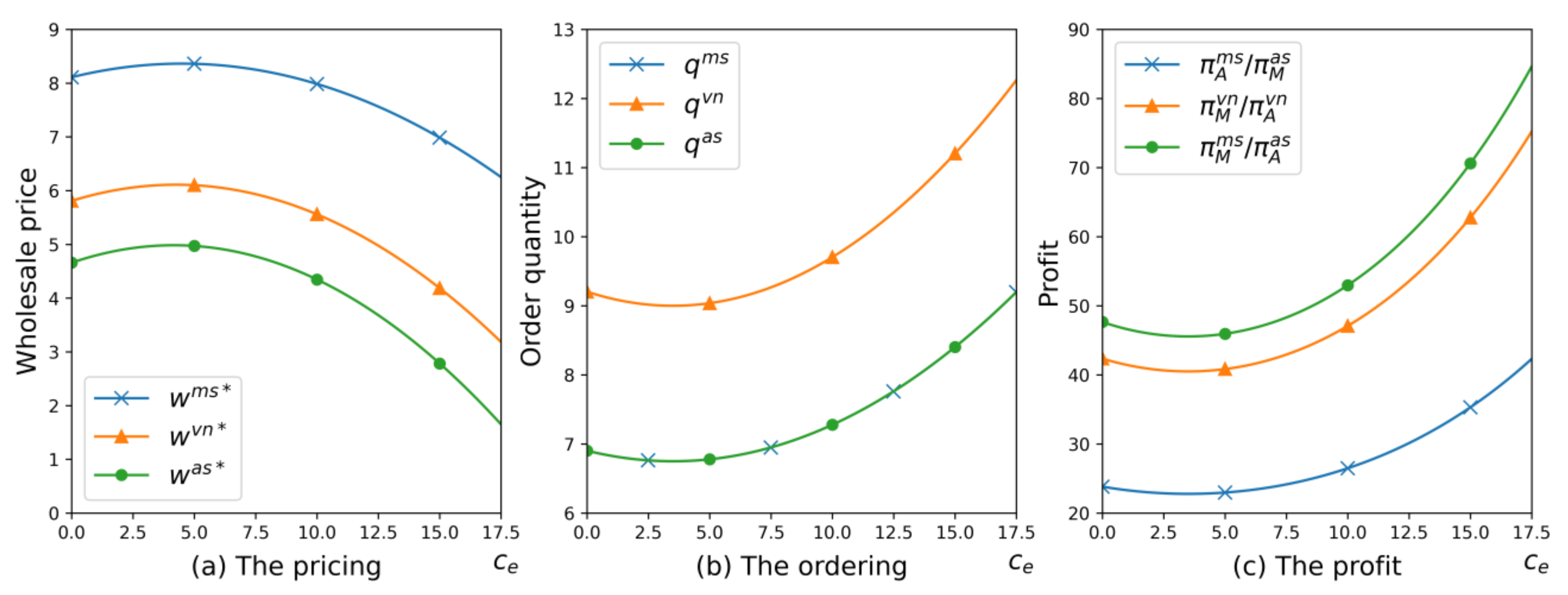
7.1. Impact of Carbon Trading Price

To gain the impact of the carbon trading price ($c_e$) on the optimal pricing ($w$), the optimal ordering ($q$), and optimal profits (${\pi }_i^j$), this paper supposed that $a=30$, $c=1.2$, $h=10$, $e_0=0.9$, $b=0.7$, $\tau =1$, $\beta =2$, and $c_e\in \left(0,20\right)$.

Figure 1 is the impact of the unit carbon trading price ($c_e$) on the optimal pricing ($w$), the optimal ordering ($q$), and the optimal profits (${\pi }_i^j$) in different power structures, and verifies Proposition 2. From Figure 1, when the unit carbon trading price is relatively low, PBM reduces emissions a little, which leads to an increase in PBM cost. The PBM increased cost brings about higher wholesale prices, leading to reduced orders from PBA, which finally results in profit loss. As the unit carbon trading price is high, PBM reduces emissions a lot, which leads to increasing the PBM revenue. The PBM increased revenue brings about lower wholesale prices and increased orders from the PBA, which finally result in a higher profit for both.

7.2. Impact of Price Sensitivity Coefficient

To gain the impact of the consumer’s price sensitivity coefficient ($\beta$) on the optimal pricing ($w$), the optimal ordering ($q$), and optimal profits (${\pi }_i^j$), there are two cases in this section. In the first case, when the carbon trading price is low, it is satisfied that $H>0$. In the second case, when the carbon trading price is high, $H<0$ is satisfied.

In the first case, it is supposed that $a=30$, $c=1.2$, $h=10$, $e_0=0.9$, $b=0.7$, $\tau =1$, $c_e=3.5$, $\beta \in \left(0,50\right)$. It is satisfied that the carbon trading price is low (i.e., $H=63.75>0$).

Figure 2 shows the sensitivity analysis of the consumer’s price sensitivity coefficient on the optimal pricing, the optimal ordering, and optimal profits in different power structures, and verifies Proposition 3 ($H>0$). Although the profits in Figure 2c decrease first and then increase as the price sensitivity coefficient increases, from Figure 2b, when the profits begin to increase ($\beta >18.93$), the order quantity is less than 0, which is not feasible in real life and contrary to our hypothesis, so the profits decrease as the price sensitivity coefficient increases in this case. In a word, when the carbon trading price is low, the high price sensitivity coefficient is bad for the supply chain, which makes the manufacture suspend production.

In the second case, it is supposed that $a=30$, $c=1.2$, $h=10$, $e_0=0.9$, $b=0.7$, $\tau =1$, $c_e=15$, and $\beta \in \left(0,50\right)$. It is satisfied that the carbon trading price is high (i.e., $H=-57<0$). Figure 3 is the sensitivity analysis of the consumer’s price sensitivity coefficient on the optimal pricing, the optimal ordering, and optimal profits in different power structures, and verifies Proposition 3 ($H<0$).

From Figure 3, when the consumer price sensitivity is high, the decrease in wholesale price and the increase in order quantity can make the profits increase. From Figure 3c, if the price sensitivity coefficient is relatively low, the smaller the price sensitivity, the higher the profits of members will be in different power structures. It is interesting that as the price sensitivity coefficient increases, there will be a situation ($\beta >21.58$ in the MS model, $\beta >10.79$ in the VN model, and $\beta >7.20$ in the AS model), where the wholesale price is less than 0 in Figure 3a. When the wholesale price is less than 0, it shows that PBM will not be able to make profits by selling prefabricated components. Instead, PBM subsidizes PBA to promote order, and sells carbon emission quotas into the market to make profits. In a word, when the unit carbon trading price is high ($H<0$), if the price sensitivity coefficient is high enough ($\beta >21.58$ in the MS model, $\beta >10.79$ in the VN model, and $\beta >7.20$ in the AS model) to make up for the loss of products sold below cost through carbon trading, PBM should subsidize PBA to increase order quantities.

7.3. Impact of Low Carbon Sensitivity Coefficient

To gain the impact of the consumer’s low carbon sensitivity coefficient ($\tau$) on the optimal pricing ($w$), optimal ordering ($q$), and optimal profits (${\pi }_i^j$), this paper supposed that $a=30$, $c=1.2$, $h=10$, $e_0=0.9$, $b=0.7$, $\beta =2$, $c_e=3.5$, and $\tau \in \left(0,29\right)$.

Figure 4 shows the sensitivity analysis of the consumer’s low carbon sensitivity coefficient ($\tau$) on the optimal pricing ($w$), optimal ordering ($q$), and optimal profits (${\pi }_i^j$) in different power structures, and verifies Proposition 4. Low carbon sensitivity has positive effects throughout the supply chain, increasing carbon reduction, pricing and ordering, and profits. The government should vigorously advocate low-carbon living and improve consumers’ awareness of low-carbon so that the whole supply chain can be greener while increasing the welfare of the supply chain members.

8. Conclusions and Future Research

The construction industry will inevitably face many new problems in the process of industrialization. Under a flexible cap-and-trade policy and power structure, this paper studies the decisions of pricing, ordering, and PBM’s emission reduction in a two-stage prefabricated building supply chain with a PBM and PBA. This paper provides a reference for prefabricated building companies to promote low-carbon transformation and achieve high-quality economic development. Our study solved the three questions in the introduction, and draws the following conclusions.

(1) The PBM and PBA make different decisions of pricing and ordering in the different power structures, but power structures can’t influence the PBM’s carbon emission reduction decision. In Stackelberg models, as a weak position, the followers always gain lower profits compared to the leaders, and we find that the followers and leaders’ profits are influenced by the pricing, not the ordering. The supply chain profit of VN model is higher than MS model and AS model. Therefore, to improve the performance of supply chain, the industry leaders should pay attention to the interests of supply chain members.

(2) The trend of the carbon trading price’s impact on the decisions are the same in different power structures. This indicates that the low unit carbon trading price leads to less carbon emission reductions and lower profit for PBA and PBM. The high unit carbon trading price increases the amount of carbon emission reduction and the profits of PBM and PBA. With the increasing carbon trading price, PBM will be forging ahead in reducing emissions and expanding production, which makes the permitted carbon emission quota a possible type of trading product to create profit for PBM and PBA.

(3) The impact of the consumer’s price sensitivity coefficient on the optimal pricing, ordering, and profits is related to the carbon trading price. When the carbon trading price is low, the high price sensitivity coefficient is bad for the supply chain, which makes PBM suspend production. When the unit carbon trading price is high, the smaller the price sensitivity is, the greater the PBM and PBA profits will be. Furthermore, when the unit carbon trading price and price sensitivity coefficient are both high enough to make up for the loss of products sold below cost through carbon trading, PBM will subsidize PBA to promote orders through the transfer of payment or revenue-sharing contracts. The low carbon sensitivity coefficient has a positive effect on the supply chain, increasing carbon reductions and profits, which are good for PBM, PBA, and the environment.

(4) The two-part tariff contract can improve the performance of the supply chain under different power structures. The distribution of profit with a two-part tariff contract is determined by the supply chain leader. This indicates that PBA and PBM will be more willing to cooperate with the two-part tariff when they choose partners with an equal market position, as they both can gain increased profit.

This paper makes contributions to the research content of prefabricated building supply chain decisions under flexible cap-and-trade. However, we did not consider the risk and uncertainty of the supply chain in our study. In real life, risk and uncertainty are becoming more and more common in prefabricated building projects, such as the uncertainty of customer demand and production lead-time. The first further research direction will be to introduce uncertainty into the optimization of the prefabricated building supply chain, such as the uncertainty of customer demand and the production lead-time. Moreover, this paper only considers the situation where the PBM has only one sales channel. In the actual situation, the PBM may assemble prefabricated buildings by itself. Another further research direction is examining the decisions of the prefabricated building industry when there are two kinds of sales channels in the market: one is the PBM direct sales channel in which the PBM manufactures and sells prefabricated buildings directly to consumers, and then assembles prefabricated buildings for consumers, and the other is the indirect sales channel in which PBM manufactures prefabricated building components and sells them to the PBA, then the PBA sells the prefabricated buildings to consumers and assembles them for consumers. In addition, this study only considers the emission reduction of the PBM and does not consider the emission reduction of the PBA. The third future research direction is to optimize the carbon emission reduction decisions of the PBM and PBA when they are both restricted by flexible cap-and-trade and need to invest in low-carbon technologies.

References

1. Soleille, S. Greenhouse gas emission trading schemes: A new tool for the environmental regulator’s kit. Energy Policy 2006, 34, 1473–1477. [Google Scholar] [CrossRef]
2. Li, W.; Zhang, Y.; Lu, C. The impact on electric power industry under the implementation of national carbon trading market in China: A dynamic CGE analysis. J. Clean. Prod. 2018, 200, 511–523. [Google Scholar] [CrossRef]
3. Ji-Feng, L.; Ya-Xiong, Z.; Xin, W.; Song-Feng, C. Policy Implications for Carbon Trading Market Establishment in China in the 12th Five-Year Period. Adv. Clim. Chang. Res. 2012, 3, 163–173. [Google Scholar] [CrossRef]
4. NDRC. Responsible Comrades of the National Development and Reform Commission Attended the 6th Annual Global Conference on Energy Efficiency. Available online: https://en.ndrc.gov.cn/news/activities/activitiespic/202105/t20210521_1280513.html (accessed on 16 September 2021).
5. Wang, S.Y.; Choi, S.H. Pareto-efficient coordination of the contract-based MTO supply chain under flexible cap-and-trade emission constraint. J. Clean. Prod. 2020, 250, 119571. [Google Scholar] [CrossRef]
6. van Roosmalen, M.; Herrmann, A.; Kumar, A. A review of prefabricated self-sufficient facades with integrated decentralised HVAC and renewable energy generation and storage. Energy Build. 2021, 248, 111107. [Google Scholar] [CrossRef]
7. Masood, R.; Lim, J.B.P.; González, V.A. Performance of the supply chains for New Zealand prefabricated house-building. Sustain. Cities Soc. 2021, 64, 102537. [Google Scholar] [CrossRef]
8. MacAskill, S.; Mostafa, S.; Stewart, R.A.; Sahin, O.; Suprun, E. Offsite construction supply chain strategies for matching affordable rental housing demand: A system dynamics approach. Sustain. Cities Soc. 2021, 73, 103093. [Google Scholar] [CrossRef]
9. Cao, X.; Li, X.; Zhu, Y.; Zhang, Z. A comparative study of environmental performance between prefabricated and traditional residential buildings in China. J. Clean. Prod. 2015, 109, 131–143. [Google Scholar] [CrossRef]
10. Wen, J.; Lanjun, W. Flow shop optimization of hybrid make-to-order and make-to-stock in precast concrete component production. J. Clean. Prod. 2021, 297, 126708. [Google Scholar]
11. Teng, Y.; Li, K.; Pan, W.; Ng, T. Reducing building life cycle carbon emissions through prefabrication: Evidence from and gaps in empirical studies. Build. Environ. 2018, 132, 125–136. [Google Scholar] [CrossRef]
12. Chang, Y.; Li, X.; Masanet, E.; Zhang, L.; Huang, Z.; Ries, R. Unlocking the green opportunity for prefabricated buildings and construction in China. Resour. Conserv. Recycl. 2018, 139, 259–261. [Google Scholar] [CrossRef]
13. Tumminia, G.; Guarino, F.; Longo, S.; Ferraro, M.; Cellura, M.; Antonucci, V. Life cycle energy performances and environmental impacts of a prefabricated building module. Renew. Sustain. Energy Rev. 2018, 92, 272–283. [Google Scholar] [CrossRef]
14. Wasim, M.; Han, T.M.; Huang, H.; Madiyev, M.; Ngo, T.D. An approach for sustainable, cost-effective and optimised material design for the prefabricated non-structural components of residential buildings. J. Build. Eng. 2020, 32, 101474. [Google Scholar] [CrossRef]
15. Li, Z.; Shen, G.Q.; Alshawi, M. Measuring the impact of prefabrication on construction waste reduction: An empirical study in China. Resour. Conserv. Recycl. 2014, 91, 27–39. [Google Scholar] [CrossRef] [Green Version]
16. Vanke. 2020 Sustainability Report. Available online: https://www.vanke.com/citizenship.aspx?type=18&id=7468 (accessed on 16 September 2021).
17. China State Construction. Building Science and Technology Business. Available online: https://en.cscec.com/Business_en/NewBusiness/ (accessed on 16 September 2021).
18. BROAD. Over 20-Year of Development, 8 Generations of High-Rise Building Product System, Over 1000 Practical Project Experiences. Available online: http://www.bhome.com.cn/en/technology/ (accessed on 16 September 2021).
19. Tang, R.; Yang, L. Impacts of financing mechanism and power structure on supply chains under cap-and-trade regulation. Transp. Res. Part E: Logist. Transp. Rev. 2020, 139, 101957. [Google Scholar] [CrossRef]
20. Chen, X.; Wang, X.; Zhou, M. Firms’ green R&D cooperation behaviour in a supply chain: Technological spillover, power and coordination. Int. J. Prod. Econ. 2019, 218, 118–134. [Google Scholar]
21. Agi, M.A.N.; Yan, X. Greening products in a supply chain under market segmentation and different channel power structures. Int. J. Prod. Econ. 2020, 223, 107523. [Google Scholar] [CrossRef]
22. Ranjbar, Y.; Sahebi, H.; Ashayeri, J.; Teymouri, A. A competitive dual recycling channel in a three-level closed loop supply chain under different power structures: Pricing and collecting decisions. J. Clean. Prod. 2020, 272, 122623. [Google Scholar] [CrossRef]
23. Xia, Q.; Zhi, B.; Wang, X. The role of cross-shareholding in the green supply chain: Green contribution, power structure and coordination. Int. J. Prod. Econ. 2021, 234, 108037. [Google Scholar] [CrossRef]
24. Kellner, F.; Schneiderbauer, M. Further insights into the allocation of greenhouse gas emissions to shipments in road freight transportation: The pollution routing game. Eur. J. Oper. Res. 2019, 278, 296–313. [Google Scholar] [CrossRef]
25. Pía, A.; Sebastián, C.; Felipe, F. A two stage cap-and-trade model with allowance re-trading and capacity investment: The case of the Chilean NDC targets. Energy 2021, 224, 120129. [Google Scholar]
26. Agi, M.A.; Faramarzi-Oghani, S.; Hazır, Ö. Game theory-based models in green supply chain management: A review of the literature. Int. J. Prod. Res. 2021, 59, 4736–4755. [Google Scholar] [CrossRef]
27. Xu, X.; He, P.; Xu, H.; Zhang, Q. Supply chain coordination with green technology under cap-and-trade regulation. Int. J. Prod. Econ. 2017, 183, 433–442. [Google Scholar] [CrossRef]
28. Xu, L.; Wang, C.; Zhao, J. Decision and coordination in the dual-channel supply chain considering cap-and-trade regulation. J. Clean. Prod. 2018, 197, 551–561. [Google Scholar] [CrossRef]
29. Zhang, S.; Wang, C.; Yu, C.; Ren, Y. Governmental cap regulation and manufacturer’s low carbon strategy in a supply chain with different power structures. Comput. Ind. Eng. 2019, 134, 27–36. [Google Scholar] [CrossRef]
30. Yang, L.; Hu, Y.; Huang, L. Collecting mode selection in a remanufacturing supply chain under cap-and-trade regulation. Eur. J. Oper. Res. 2020, 287, 480–496. [Google Scholar] [CrossRef]
31. Yu, S.; Liu, Y.; Wang, D.; Bahaj, A.S.; Wu, Y.; Liu, J. Review of thermal and environmental performance of prefabricated buildings: Implications to emission reductions in China. Renew. Sustain. Energy Rev. 2021, 137, 110472. [Google Scholar] [CrossRef]
32. Liu, G.; Yang, H.; Fu, Y.; Mao, C.; Xu, P.; Hong, J.; Li, R. Cyber-physical system-based real-time monitoring and visualization of greenhouse gas emissions of prefabricated construction. J. Clean. Prod. 2020, 246, 119059. [Google Scholar] [CrossRef]
33. Bortolini, R.; Formoso, C.T.; Viana, D.D. Site logistics planning and control for engineer-to-order prefabricated building systems using BIM 4D modeling. Autom. Constr. 2019, 98, 248–264. [Google Scholar] [CrossRef]
34. Yao, F.; Ji, Y.; Tong, W.; Li, H.X.; Liu, G. Sensing technology based quality control and warning systems for sleeve grouting of prefabricated buildings. Autom. Constr. 2021, 123, 103537. [Google Scholar] [CrossRef]
35. Arashpour, M.; Bai, Y.; Aranda-Mena, G.; Bab-Hadiashar, A.; Hosseini, R.; Kalutara, P. Optimizing decisions in advanced manufacturing of prefabricated products: Theorizing supply chain configurations in off-site construction. Autom. Constr. 2017, 84, 146–153. [Google Scholar] [CrossRef]
36. Jiang, W.; Wu, L.; Cao, Y. Multiple Precast Component Orders Acceptance and Scheduling. Math. Probl. Eng. 2020, 1–15. [Google Scholar] [CrossRef]
37. Zhu, A.; Pauwels, P.; De Vries, B. Smart component-oriented method of construction robot coordination for prefabricated housing. Autom. Constr. 2021, 129, 103778. [Google Scholar] [CrossRef]
38. Dallasega, P.; Rojas, R.A.; Bruno, G.; Rauch, E. An agile scheduling and control approach in ETO construction supply chains. Comput. Ind. 2019, 112, 103122. [Google Scholar] [CrossRef]
39. Ekanayake, E.M.A.C.; Shen Geoffrey, Q.P.; Kumaraswamy, M. Identifying supply chain capabilities of construction firms in industrialized construction. Prod. Plan. Control. 2021, 32, 303–321. [Google Scholar] [CrossRef]
40. Han, Y.; Skibniewski, M.; Wang, L. A Market Equilibrium Supply Chain Model for Supporting Self-Manufacturing or Outsourcing Decisions in Prefabricated Construction. Sustainability 2017, 9, 2069. [Google Scholar] [CrossRef] [Green Version]
41. Zhai, Y.; Zhong, R.Y.; Huang, G.Q. Buffer space hedging and coordination in prefabricated construction supply chain management. Int. J. Prod. Econ. 2018, 200, 192–206. [Google Scholar] [CrossRef]
42. Zhai, Y.; Choi, T.M.; Shao, S.; Xu, S.X.; Huang, G.Q. Spatial-temporal hedging coordination in prefabricated housing production. Int. J. Prod. Econ. 2020, 229, 107792. [Google Scholar] [CrossRef]
43. Ghosh, D.; Shah, J. A comparative analysis of greening policies across supply chain structures. International J. Prod. Econ. 2012, 135, 568–583. [Google Scholar] [CrossRef]
44. Liu, Z.L.; Anderson, T.D.; Cruz, J.M. Consumer environmental awareness and competition in two-stage supply chains. Eur. J. Oper. Res. 2012, 218, 602–613. [Google Scholar] [CrossRef]
Figure 1. Impact of carbon trading price in different power structures: (a) impact of carbon trading price on the pricing; (b) impact of carbon trading price on the ordering; (c) impact of carbon trading price on the profit.
Mathematics 09 02426 g001
Figure 2. Impact of the consumer’s price sensitivity coefficient when the price sensitivity coefficient is low: (a) impact of the consumer’s price sensitivity coefficient on the pricing; (b) impact of the consumer’s price sensitivity coefficient on the ordering; (c) impact of the consumer’s price sensitivity coefficient on the profit.
Mathematics 09 02426 g002
Figure 3. Impact of the consumer’s price sensitivity coefficient when the price sensitivity coefficient is high: (a) impact of the consumer’s price sensitivity coefficient on the pricing; (b) impact of the consumer’s price sensitivity coefficient on the ordering; (c) impact of the consumer’s price sensitivity coefficient on the profit.
Mathematics 09 02426 g003
Figure 4. Impact of the consumer’s low carbon sensitivity coefficient in different power structures: (a) impact of the consumer’s low carbon sensitivity coefficient on the pricing; (b) impact of the consumer’s low carbon sensitivity coefficient on the ordering; (c) impact of the consumer’s low carbon sensitivity coefficient on the profit.
Mathematics 09 02426 g004