Mathematical Modeling of Immune Responses against SARS-CoV-2 Using an Ensemble Kalman Filter

Abstract

In this paper, a mathematical model was developed to simulate SARS-CoV-2 dynamics in infected patients. The model considers both the innate and adaptive immune responses and consists of healthy cells, infected cells, viral load, cytokines, natural killer cells, cytotoxic T-lymphocytes, B-lymphocytes, plasma cells, and antibody levels. First, a mathematical analysis was performed to discuss the model’s equilibrium points and compute the basic reproduction number. The accuracy of such mathematical models may be affected by many sources of uncertainties due to the incomplete representation of the biological process and poorly known parameters. This may strongly limit their performance and prediction skills. A state-of-the-art data assimilation technique, the ensemble Kalman filter (EnKF), was then used to enhance the model’s behavior by incorporating available data to determine the best possible estimate of the model’s state and parameters. The proposed assimilation system was applied on the real viral load datasets of six COVID-19 patients. The results demonstrate the efficiency of the proposed assimilation system in improving the model predictions by up to $40\%$.

1. Introduction

Since being first identified in the late fall of 2019, the outbreak of coronavirus disease (COVID-19) has received increasing attention among the scientists all over the world in order to understand the epidemiology of the disease and curb the spread of the virus. COVID-19 is a contagious disease caused by the current severe acute respiratory syndrome coronavirus 2 (SARS-CoV-2). Infected people will experience mild to moderate symptoms such as a cough, headache, fever, and in some cases, severe pneumonia [1,2]. The development of a vaccine to end the disease has undergone significant progress during the last two years. However, the virus is still going on, as the mortality rate and daily confirmed cases remain high in many countries. As efforts to eradicate the disease continue, in addition to biological and medical research, mathematical models have been suggested to play a vital role in describing and forecasting disease transmission, as well as help to implement efficient measures and strategies to control the spread of the pandemic and reduce its impact [3].

Several models have recently been proposed and implemented in order to understand the dynamics of COVID-19. Most of these models are based on the traditional epidemiological model, called the susceptible–exposed–infectious–recovered (SEIR) model, which was introduced to study the pandemic transmission within a human community [4,5,6,7,8,9,10,11,12,13,14]. To date, very few attempts have been devoted to describe the interaction between the immune system and SARS-CoV-2 [15,16,17,18]. An important limitation of these models is the presence of several sources of uncertainties, which may strongly degrade their prediction performance and lead to large inaccuracies in their outputs. Aside from the incomplete description of the biological processes, the poor characterization of the model parameters is also considered a major source of uncertainty. Therefore, it is crucial to quantify and reduce the model’s uncertainties before using them for decision making.

Data assimilation techniques provide efficient tools for quantifying and reducing the uncertainties of such models [19,20]. They constrain prior information about the state and parameters of the underlying dynamical system with available data to compute posterior updated estimates of the parameters and state variables [21], based upon which improved predictions can be obtained with the model. This process, which finds its roots in the atmospheric and oceanic weather communities, sequentially nudges model predictions towards incoming observations, so the model trajectory remains as close as possible to the true trajectory [22]. The ensemble Kalman filter (EnKF) is an efficient data assimilation technique that has been successfully implemented in many fields including atmospheric and oceanic weather forecasting [23,24,25,26,27], hydrology and reservoir applications [28,29,30,31], and flood modeling [32,33]. EnKF is a Monte Carlo implementation of the classical linear Kalman filter (KF) [34], operating with cycles of forecast and update steps. In the forecast step, a set of members sampled from the state probability distribution were integrated forward in time with the model. In the update step, a Gaussian Kalman update is applied, once a new datum becomes available [35], from which the next assimilation cycle is initiated [22,35]. Unlike the KF, the EnKF can efficiently handle model nonlinearities without the need to compute tangent linear approximations of the model as for the extended Kalman filter.

In this work, we propose a mathematical model for the innate and adaptive immune responses against SARS-CoV-2 infection. First, we conducted a mathematical analysis to derive the basic reproduction number and discuss the equilibrium states of the model. To improve the model prediction skill, an efficient state–parameters estimation framework based on a joint-EnKF assimilation scheme was developed. By considering uncertainties in the model state variables and poorly known parameters, the proposed ensemble data assimilation system updates both state and parameters ensembles every time a new observation become available. This methodology was validated with real SARS-CoV-2 viral load data obtained from a hospital in Munich. We assessed the sensitivity of the system to the ensemble size and particularly focused on the relevance of the joint-EnKF for improving the prediction capability of the immune response mathematical model.

The rest of the study is organized as follows. Section 2 presents the mathematical model and briefly outlines the joint-EnKF algorithm. Section 3 is dedicated to the mathematical analysis of the model. The numerical results are presented and discussed in Section 4. Key findings and conclusions are summarized in Section 5.

2. Model and Assimilation Scheme

2.1. Mathematical Model

The mathematical model describes the interaction dynamics of both the human innate and adaptive immune system with SARS-CoV-2 as follows. Healthy cells $H\left(t\right)$ become infected at a rate $\beta$. The virus $V\left(t\right)$ is produced by infected cells at a rate $k_1$. The innate immune system instantly responds after the viral infection. Cytokines $C\left(t\right)$ are a crucial element of the innate system and play a major role in inhibiting the viral replication at a rate $p_2$. Specific cytokines activate natural killer cells $N\left(t\right)$ at a rate r, which play an essential role in eliminating infected cells at a rate $p_5$. At the same time, cytokines activate the adaptive immune system, particularly the cytotoxic T-lymphocytes $T\left(t\right)$ at a rate ${\lambda }_1$. T-cells kill virus infected cells at a rate $p_1$ and afterwards activate B-lymphocytes $B\left(t\right)$ at a rate ${\lambda }_2$. A ratio k of B-cells differentiate into plasma cells in an antigen-dependent manner to produce antibodies at a rate $\eta$. They specifically recognize and neutralize the virus at a rate $p_3$. A schematic diagram characterizing the proposed model is presented in Figure 1. Finally, the system describing these interactions is expressed as a set of ordinary differential equations:

$$\begin{array}{cc}\hfill {\displaystyle \frac{dH\left(t\right)}{dt}}& =\mathrm{\Pi }-\beta H\left(t\right)V\left(t\right)-{\mu }_{1}H\left(t\right),\hfill \\ \hfill {\displaystyle \frac{dI\left(t\right)}{dt}}& =\beta H\left(t\right)V\left(t\right)-p_{1}T\left(t\right)I\left(t\right)-p_{5}N\left(t\right)I\left(t\right)-{\mu }_{2}I\left(t\right),\hfill \\ \hfill {\displaystyle \frac{dV\left(t\right)}{dt}}& =k_{1}I\left(t\right)-p_{2}C\left(t\right)V\left(t\right)-p_{3}A\left(t\right)V\left(t\right)-{\mu }_{3}V\left(t\right),\hfill \\ \hfill {\displaystyle \frac{dC\left(t\right)}{dt}}& =k_{2}I\left(t\right)-{\mu }_{4}C\left(t\right),\hfill \\ \hfill {\displaystyle \frac{dN\left(t\right)}{dt}}& =rC\left(t\right)-{\mu }_{5}N\left(t\right),\hfill \\ \hfill {\displaystyle \frac{dT\left(t\right)}{dt}}& ={\lambda }_{1}C\left(t\right)T\left(t\right)-{\mu }_{6}T\left(t\right),\hfill \\ \hfill {\displaystyle \frac{dB\left(t\right)}{dt}}& ={\lambda }_{2}T\left(t\right)B\left(t\right)-{\mu }_{7}B\left(t\right),\hfill \\ \hfill {\displaystyle \frac{dP\left(t\right)}{dt}}& =kB\left(t\right)V\left(t\right)-{\mu }_{8}P\left(t\right),\hfill \\ \hfill {\displaystyle \frac{dA\left(t\right)}{dt}}& =G\left(t-\tau \right)\eta P\left(t\right)-p_{4}A\left(t\right)V\left(t\right)-{\mu }_{9}A\left(t\right),\hfill \end{array}$$

(1)

where G is the Heaviside step function defined as follows:

$$G\left(t-\tau \right)=\left\{\begin{array}{cc}0\hfill & \mathrm{if}t<\tau \hfill \\ 1\hfill & \mathrm{if}t>\tau \hfill \end{array}\right.,$$

(2)

where the time delay $\tau$ is the time required to produce antibodies from plasma cells. Detailed descriptions and definitions of all the model state and parameters are given in

Table 1. Initial model variables and parameters and their biological interpretations.

Variable	InitialValue	Description	Reference
H	$4\times {10}^5$ cells per mL	Healthy cells	[36]
I	$3\times {10}^{-4}$ cells per mL	Infected cells	[36]
V	357 RNA per mL	Viral load	[36]
C	0 cells per mL	Cytokines	[16]
N	100 cells per mL	Natural killer cells	[16]
T	500 cells per mL	T-cells	[16]
B	100 cells per mL	B-cells	[16]
P	0 cells per mL	Plasma cells	[36]
A	0 molecules per ml	Antibodies level	[36]
Parameter	Initial value	Description	Reference
$\mathrm{\Pi }$	$4\times {10}^3$ cells mL${}^{-1}$ day${}^{-1}$	Production rate of healthy cells	[37]
$\beta$	$1.5\times {10}^{-7}$ mL (RNA copies)${}^{-1}$ day${}^{-1}$	Rate at which healthy cells are infected	[17]
$p_1$	$0.001$ mL cells${}^{-1}$ day${}^{-1}$	Rate at which T-cells destroy infected cells	[38]
$p_2$	(0–1) mL cells${}^{-1}$ day${}^{-1}$	Rate at which viral particles are neutralized by cytokines	[16]
$p_3$	(0–1) mL molecules${}^{-1}$ day${}^{-1}$	Rate at which viral particles are neutralized by antibodies	[16]
$p_4$	$3\times {10}^{-7}$ mL (RNA copies)${}^{-1}$ day${}^{-1}$	Rate at which virus neutralizes antibodies	[36]
$p_5$	$5.74\times {10}^{-4}$ mL cells${}^{-1}$ day${}^{-1}$	Rate at which infected cells are diminished by NK cells	[39]
k	${10}^{-5}$ mL (RNA copies)${}^{-1}$ day${}^{-1}$	Plasma cells recruitment	[36]
$k_1$	(8.2–525) day${}^{-1}$	Production rate of virus from infected cells	[17]
$k_2$	(0–10) day${}^{-1}$	Production rate of cytokines	[16]
r	$0.52$ day${}^{-1}$	Activation rate of NK cells	[39]
${\lambda }_1$	$0.1$ mL cells${}^{-1}$ day${}^{-1}$	Activation rate of T cells	[40]
${\lambda }_2$	$0.01$ mL cells${}^{-1}$ day${}^{-1}$	Activation rate of B cells	[40]
$\eta$	(0–1) day${}^{-1}$	Antibodies production rate	[41]
${\mu }_1$	$0.14$ day${}^{-1}$	Natural death rate of healthy cells and protected cells	[40]
${\mu }_2$	(0–1) day${}^{-1}$	Natural death rate of infected cells	[16]
${\mu }_3$	(0–1) day${}^{-1}$	Clearance rate of virus	[16]
${\mu }_4$	$0.7$ day${}^{-1}$	Natural death rate of cytokines	[16]
${\mu }_5$	$0.07$ day${}^{-1}$	Natural death rate of NK cells	[39]
${\mu }_6$	1 day${}^{-1}$	Natural death rate of T cells	[40]
${\mu }_7$	$0.2$ day${}^{-1}$	Natural death rate of B cells	[36]
${\mu }_8$	4 day${}^{-1}$	Natural death rate of plasma cells	[18]
${\mu }_9$	$0.07$ day${}^{-1}$	Natural death rate of antibodies	[40]
$\tau$	7–14 days	Time delay for antibody production	[16]

.

2.2. Ensemble Kalman Filter (EnKF)

Consider the following space–time dynamical system:

$$\begin{array}{cc}\hfill {\mathbf{x}}_{k+1}& =\mathcal{M}\left({\mathbf{x}}_k,\theta \right)+{\eta }_{k+1},\hfill \\ \hfill {\mathbf{y}}_{k+1}& =\mathcal{H}\left({\mathbf{x}}_{k+1}\right)+{ϵ}_{k+1},\hfill \end{array}$$

(3)

where the model’s prognostic state is denoted by ${\mathbf{x}}_k$, $\mathcal{M}$ is the nonlinear predictive model and $\theta$ denotes a set of modeling parameters. The observations at time $t_{k+1}$ are given by ${\mathbf{y}}_{k+1}$. The state variables are mapped into the observation space using the $\mathcal{H}$ operator. Model errors ${\eta }_{k+1}$ are assumed Gaussian, centered at zero with a prescribed covariance ${\mathbf{Q}}_{k+1}$. Observation errors ${ϵ}_{k+1}$, on the other hand, are assumed to be uncorrelated with the model errors and further follow $\mathcal{N}\left(0,{\mathbf{R}}_{k+1}\right)$.

During the forecast step, the model is used to integrate an ensemble of states forward in time. The prior sample mean and covariance are then approximated as

$${\widehat{\mathbf{x}}}_{k+1}^f={\displaystyle \frac{1}{N_e}}\sum _{i=1}^{N_e}{\mathbf{x}}_{k+1}^{f,i},$$

(4)

$${\widehat{\mathbf{P}}}_{k+1}^f={\displaystyle \frac{1}{N_e-1}}\sum _{i=1}^{N_e}\left({\mathbf{x}}_{k+1}^{f,i}-{\widehat{\mathbf{x}}}_{k+1}^f\right){\left({\mathbf{x}}_{k+1}^{f,i}-{\widehat{\mathbf{x}}}_{k+1}^f\right)}^T={\mathbf{X}}_{k+1}^f{\left({\mathbf{X}}_{k+1}^f\right)}^T,$$

(5)

where $N_e$ is the ensemble size.

By augmenting the state and parameters—${\mathbf{z}}_{k+1}=\left[{\mathbf{x}}_{k+1}^T,{\mathsf{\theta }}^T\right]$—the joint-EnKF uses $y_{k+1}$ to update the prior joint state as follows:

$${\mathbf{z}}_{k+1}^f=\tilde{\mathcal{M}}\left({\mathbf{z}}_k,\mathsf{\theta }\right)+{\eta }_{k+1}=\left[\begin{array}{c}\mathcal{M}\left({\mathbf{x}}_k,\mathsf{\theta }\right)+{\eta }_{k+1}\\ \mathsf{\theta }\end{array}\right],$$

(6)

such that $\tilde{\mathcal{M}}$ is a modified nonlinear function operating on the augmented state–parameters vector. Using the ensemble members of both the state and parameters, the joint prior covariance can be formed as

$${\widehat{\mathbf{P}}}_{k+1}^f=\left[\begin{array}{c}{\widehat{\mathbf{P}}}_{{\mathbf{x}}_{k+1}{\mathbf{x}}_{k+1}}^f{\widehat{\mathbf{P}}}_{{\mathbf{x}}_{k+1}{\mathsf{\theta }}_{k+1}}^f\\ {\widehat{\mathbf{P}}}_{{\mathsf{\theta }}_{k+1}{\mathbf{x}}_{k+1}}^f{\widehat{\mathbf{P}}}_{{\mathsf{\theta }}_{k+1}{\mathsf{\theta }}_{k+1}}^f\end{array}\right]=\left[\begin{array}{c}{\mathbf{X}}_{{\mathbf{x}}_{k+1}}^f{\left({\mathbf{X}}_{{\mathbf{x}}_{k+1}}^f\right)}^T{\mathbf{X}}_{{\mathbf{x}}_{k+1}}^f{\left(X_{{\mathsf{\theta }}_{k+1}}^f\right)}^T\\ {\mathbf{X}}_{{\mathsf{\theta }}_{k+1}}^f{\left({\mathbf{X}}_{{\mathbf{x}}_{k+1}}^f\right)}^T{\mathbf{X}}_{{\mathsf{\theta }}_{k+1}}^f{\left({\mathbf{X}}_{{\mathsf{\theta }}_{k+1}}^f\right)}^T\end{array}\right],$$

(7)

where ${\mathbf{X}}_{\theta }$ represents the departure of the parameter ensemble from the mean, i.e., ensemble anomalies. A linear Kalman update is applied to compute the analysis state and parameter ensembles:

$$\left(\begin{array}{c}{\mathbf{x}}_{k+1}^{a,i}\\ {\mathsf{\theta }}_{k+1}^{a,i}\end{array}\right)=\left(\begin{array}{c}{\mathbf{x}}_{k+1}^{f,i}\\ {\mathsf{\theta }}_{k+1}^{f,i}\end{array}\right)+\left(\begin{array}{c}{\mathbf{X}}_{{\mathbf{x}}_{k+1}}^f\\ {\mathbf{X}}_{{\mathsf{\theta }}_{k+1}}^f\end{array}\right)·{\mathbf{w}}_i,$$

(8)

where ${\mathbf{w}}_i={\left(\mathcal{H}{\mathbf{X}}_{{\mathbf{x}}_{k+1}}^f\right)}^T{\left[\left(\mathcal{H}{\mathbf{X}}_{{\mathbf{x}}_{k+1}}^f\right){\left(\mathcal{H}{\mathbf{X}}_{{\mathbf{x}}_{k+1}}^f\right)}^T+R\right]}^{-1}·\left({\mathbf{y}}_{k+1}^i-\mathcal{H}{\mathbf{x}}_{k+1}^{f,i}\right)$.

3. Mathematical Analysis of the Immune Response Model

This section discusses the equilibrium states, the stability of the disease-free equilibrium, and the basic reproduction number of the immune response model (1).

3.1. Disease-Free Equilibrium and Basic Reproduction Number of the Model

Model (1) has a unique disease-free equilibrium $X_0$ obtained by setting all the right-hand side to zero with $V=0$ as follows:

$$X_0=\left({\displaystyle \frac{\mathrm{\Pi }}{{\mu }_1}},0,0,0,0,0,0,0,0\right).$$

(9)

The basic reproduction number $R_0$ represents the average number of secondary infected cells produced by a single infected cell in the infection-free environment. We calculated it using the next-generation method [42]. Let F and W denote the matrix of the new infection and the transmission matrix, respectively. At the disease-free equilibrium $X_0$, F and W are given by

$$F=\left(\begin{array}{cc}0& \beta \mathrm{\Pi }/{\mu }_1\\ 0& 0\end{array}\right),W=\left(\begin{array}{cc}{\mu }_2& 0\\ -k_1& {\mu }_3\end{array}\right).$$

(10)

Following [42], the basic reproduction number $R_0$ is the dominant eigenvalue of the next-generation matrix $F{W}^{-1}$, so that:

$$R_0={\displaystyle \frac{\mathrm{\Pi }\beta k_1}{{\mu }_1{\mu }_2{\mu }_3}}.$$

(11)

3.2. Analysis of the Steady States

Model (1) has four steady states:

• The disease-free equilibrium $X_0$.
• The virus persistence equilibrium in the absence of immune responses given by

  $$X_1=\left(H_1,I_1,V_1,0,0,0,0,0,0\right),$$

  (12)

  where:

  $$H_1={\displaystyle \frac{\mathrm{\Pi }}{{\mu }_1{R}_0}},I_1={\displaystyle \frac{{\mu }_1{\mu }_3\left(R_0-1\right)}{\beta k_1}},V_1={\displaystyle \frac{{\mu }_1\left(R_0-1\right)}{\beta }}.$$

  (13)

We can clearly see that the equilibrium $X_1$ exists when $R_0>1$.

3.

The virus persistence equilibrium in the absence of the adaptive immune response given by

$$X_2=\left(H_2,I_2,V_2,C_2,N_2,0,0,0,0\right),$$

(14)

where:

$$H_2={\displaystyle \frac{\mathrm{\Pi }}{\beta V_2+{\mu }_1}},I_2={\displaystyle \frac{{\mu }_4{C}_2}{k_2}},V_2={\displaystyle \frac{k_1{\mu }_4{C}_2}{k_2\left(p_2{C}_2+{\mu }_3\right)}},N_2={\displaystyle \frac{r{C}_2}{{\mu }_5}},$$

(15)

and $C_2$ is the root of the quadratic equation:

$$a_2{C}_2^2+a_1{C}_2+a_0=0,$$

(16)

with:

$$a_0={\displaystyle \frac{{\mu }_5{k}_2\left(1-R_0\right)}{{\mu }_1{\mu }_2{\mu }_3}},a_2=r{p}_5\left(\beta {\mu }_4{k}_1+{\mu }_1{k}_2{p}_2\right).$$

(17)

It is clear that $a_2$ is always positive, therefore, Equation (16) has a unique positive solution when $a_0<0$. Thus, $R_0>1$ ensures the existence of $X_2$.

4.

The all cells and virus co-existence equilibrium is given by

$$X_3=\left(H_3,I_3,V_3,C_3,N_3,T_3,B_3,P_3,A_3\right),$$

(18)

where:

$$T_3={\displaystyle \frac{{\mu }_7}{{\lambda }_2}},C_3={\displaystyle \frac{{\mu }_6}{{\lambda }_1}},N_3={\displaystyle \frac{r{\mu }_6}{{\lambda }_1{\mu }_5}},I_3={\displaystyle \frac{{\mu }_4{\mu }_6}{k_2{\lambda }_1}}.$$

(19)

From the first equation of system (1), one has:

$$H_3={\displaystyle \frac{\mathrm{\Pi }}{\beta V_3+{\mu }_1}},$$

(20)

and from the third one:

$$V_3={\displaystyle \frac{k_{1}I}{p_2{C}_3+p_3{A}_3+{\mu }_3}}.$$

(21)

Putting the expressions of $H_3$ and $V_3$ into the second equation of system (1), we obtain the following expression for $A_3$:

$$A_3={\displaystyle \frac{{\mu }_1{\mu }_2{\mu }_3\left(R_0-R_1-1\right)}{{\mu }_1{p}_3{p}_5{N}_3+{\mu }_1{p}_1{p}_3{T}_3+{\mu }_1{\mu }_2{p}_3}},$$

(22)

where:

$$R_1={\displaystyle \frac{\left(p_5{N}_3+p_1{T}_3+{\mu }_2\right)\left(\beta k_1{I}_3+{\mu }_1{p}_2{C}_3\right)+{\mu }_1{\mu }_3\left(p_5{N}_3+p_1{T}_3\right)}{{\mu }_1{\mu }_2{\mu }_3}}.$$

(23)

Finally, the last two equations of system (1) give:

$$P_3={\displaystyle \frac{p_4{A}_3{V}_3+{\mu }_9{A}_3}{G(t-\tau )\eta }},B_3={\displaystyle \frac{{\mu }_8{P}_3}{{\lambda }_3{V}_3}}.$$

(24)

Since $X_3$ should be positive, one can see that the equilibrium $X_3$ exists if $R_0>R_1+1$.

Theorem 1.

The disease-free equilibrium $X^0$ is locally asymptotically stable when $R_0<1$, and unstable when $R_0>1$.

Proof of Theorem 1. 

The Jacobian matrix of the model (1) at the disease-free equilibrium is defined as

$$J\left(X^0\right)=\left(\begin{array}{ccccccccc}-{\mu }_1& 0& -\beta \mathrm{\Pi }/{\mu }_1& 0& 0& 0& 0& 0& 0\\ 0& -{\mu }_2& \beta \mathrm{\Pi }/{\mu }_1& 0& 0& 0& 0& 0& 0\\ 0& k_1& -{\mu }_3& 0& 0& 0& 0& 0& 0\\ 0& k_2& 0& -{\mu }_4& 0& 0& 0& 0& 0\\ 0& 0& 0& r& -{\mu }_5& 0& 0& 0& 0\\ 0& 0& 0& 0& 0& -{\mu }_6& 0& 0& 0\\ 0& 0& 0& 0& 0& 0& -{\mu }_7& 0& 0\\ 0& 0& 0& 0& 0& 0& 0& -{\mu }_8& 0\\ 0& 0& 0& 0& 0& 0& 0& G(t-\tau )\eta & -{\mu }_9\end{array}\right).$$

(25)

Clearly, $J\left(X^0\right)$ has the eigenvalues ${\lambda }_1=-{\mu }_1$, ${\lambda }_2=-{\mu }_4$, ${\lambda }_3=-{\mu }_5$, ${\lambda }_4=-{\mu }_6$, ${\lambda }_5=-{\mu }_7$, ${\lambda }_6=-{\mu }_8$, and ${\lambda }_7=-{\mu }_9$, which are all negative. The other two eigenvalues ${\lambda }_8$ and ${\lambda }_9$ are solutions of the quadratic equation ${\lambda }^2+a_1\lambda +a_0=0$, where:

$$a_0={\mu }_2{\mu }_3\left(1-R_0\right),a_1={\mu }_2+{\mu }_3.$$

(26)

$a_1$ is always positive and for $R_0<1$, $a_0$ becomes also positive. By the Routh–Hurwitz condition, the last two eigenvalues ${\lambda }_8$ and ${\lambda }_9$ are negative. Hence, the disease-free equilibrium $X^0$ is locally asymptotically stable when $R_0<1$. For the case $R_0>1$, $a_0$ becomes negative and one of the two eigenvalues ${\lambda }_8$ and ${\lambda }_9$ is positive. Therefore, whenever $R_0>1$, the disease-free equilibrium $X^0$ is unstable [43]. □

4. Results and Discussion

The aforementioned model is applied to forecast the SARS-CoV-2 viral load. Real data including daily viral load measurements from six patients in a hospital in Munich (Germany) are obtained from [44]. The assimilation impact is assessed by comparing the data assimilation output obtained using the joint-EnKF to those of the model free-run without assimilation.

4.1. Assimilation Settings

The state vector $\left(\mathbf{x}\right)$ to be assimilated includes nine variables: the number of healthy cells H, infected cells I, viral load V, cytokines C, natural killer cells N, cytotoxic T-lymphocytes T, B-lymphocytes B, plasma cells P and antibody levels A:

$$\mathbf{x}=\left[HIVCNTBPA\right],$$

(27)

and the parameters vector $\left(\mathsf{\theta }\right)$ contains all model parameters listed in Table 1, meaning that:

$$\mathsf{\theta }=\left[\mathrm{\Pi }\beta p_1{p}_2{p}_3{p}_4{p}_{5}k{k}_1{k}_{2}r{\lambda }_1{\lambda }_2\eta {\mu }_1{\mu }_2{\mu }_3{\mu }_4{\mu }_5{\mu }_6{\mu }_7{\mu }_8{\mu }_9\tau \right].$$

(28)

In the joint-EnK, the state and parameters are simultaneously estimated. Thus, the augmented state vector becomes:

$$\mathbf{z}=\left[{\mathbf{x}}^{T}log\left({\mathsf{\theta }}^T\right)\right].$$

(29)

To prevent negative input, all parameters are taken in a logarithmic form during the estimation procedure. The total number of estimated variables by the joint state is 33.

The initial state and parameter values are outlined in Table 1 with $p_2=0.001$, $p_3=0.05$, $k_1=379$, $k_2=5$, $\eta =0.05$, ${\mu }_2=0.65$, ${\mu }_3=0.9$, and $\tau =7$. To initialize the simulation, the state ensemble at time zero is drawn from a truncated Gaussian distribution using the initial state $x_0$ as:

$${\mathbf{x}}_0^i=max\left[x_0+\left(\kappa x_0\right)\sigma ,0\right],i=1,2,\dots ,N_e.$$

(30)

A preprocessing step is performed to ensure all initial state variables are non-negative. The standard deviation of the initial ensemble distribution is chosen as $\kappa x_0$, where $\kappa =10\%$ and $\sigma$ is a standard normal distribution. Likewise, the parameter ensemble is initialized starting from the nominal parameters of Table 1 in which a log-normal distribution, with a $10\%$ standard deviation, is used to draw the parameter samples. A larger initial uncertainty range is assigned to parameter $\beta$ where the standard deviation is set to $40\%$. To prescribe the uncertainty in the data, the observation error covariance at any time $t_k$ is assumed diagonal (i.e., observations error correlations in space vanish) with variances set to $5\%$ of the data values.

The prediction skill of the data assimilation framework is evaluated using the following relative absolute error (RAE):

$$\mathrm{RAE}={\displaystyle \frac{{\sum }_{k=1}^K|y^o\left(k\right)-y^f\left(k\right)|}{{\sum }_{k=1}^K\left|y^o\left(k\right)\right|}},$$

(31)

where $y^o\left(k\right)$ denotes the $k^{\mathrm{th}}$ value of the observed data, $y^f\left(k\right)$ is the associated forecast mean and K is the sample size of the observed data at that time.

4.2. Sensitivity to Ensemble Size

Initially, we investigated the EnKF sensitivity to the ensemble size $N_e$, which is a key feature of the EnKF. Running the filter using large ensemble sizes is undoubtedly more costly. Therefore, computing reliable state and parameter estimation using small ensembles is often desired. We run the assimilation system using six ensembles with different sizes varying from $N_e=25$ to 1000, and report the average RAE of the forecasted viral load in Figure 2. As expected, increasing the ensemble size improves the performance of the filter. As shown in Figure 2, the use of 100 ensemble members leads to a nearly $35\%$ decrease in the RAE compared to using 25 members. However, increasing the ensemble size beyond 100 only has a marginal effect on the accuracy (roughly $6\%$) relative to the increment in the runtime cost. Therefore, we run the rest of our simulations with 100 members.

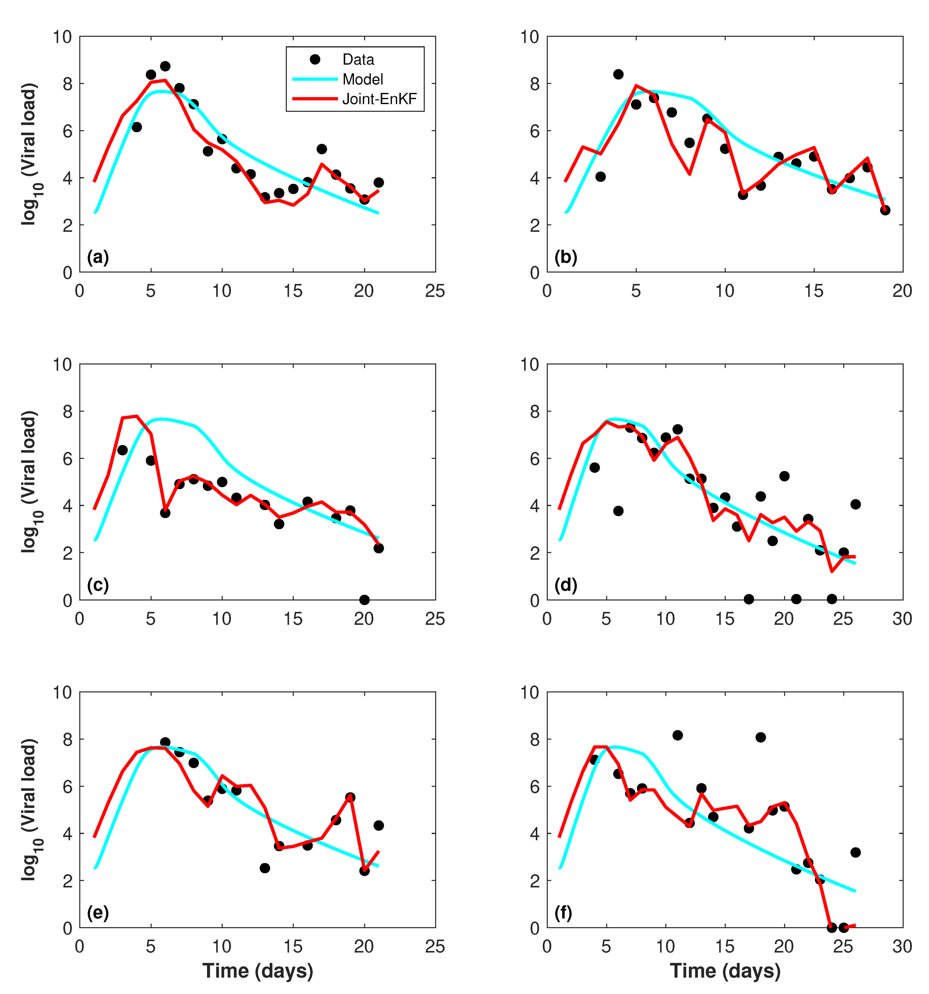
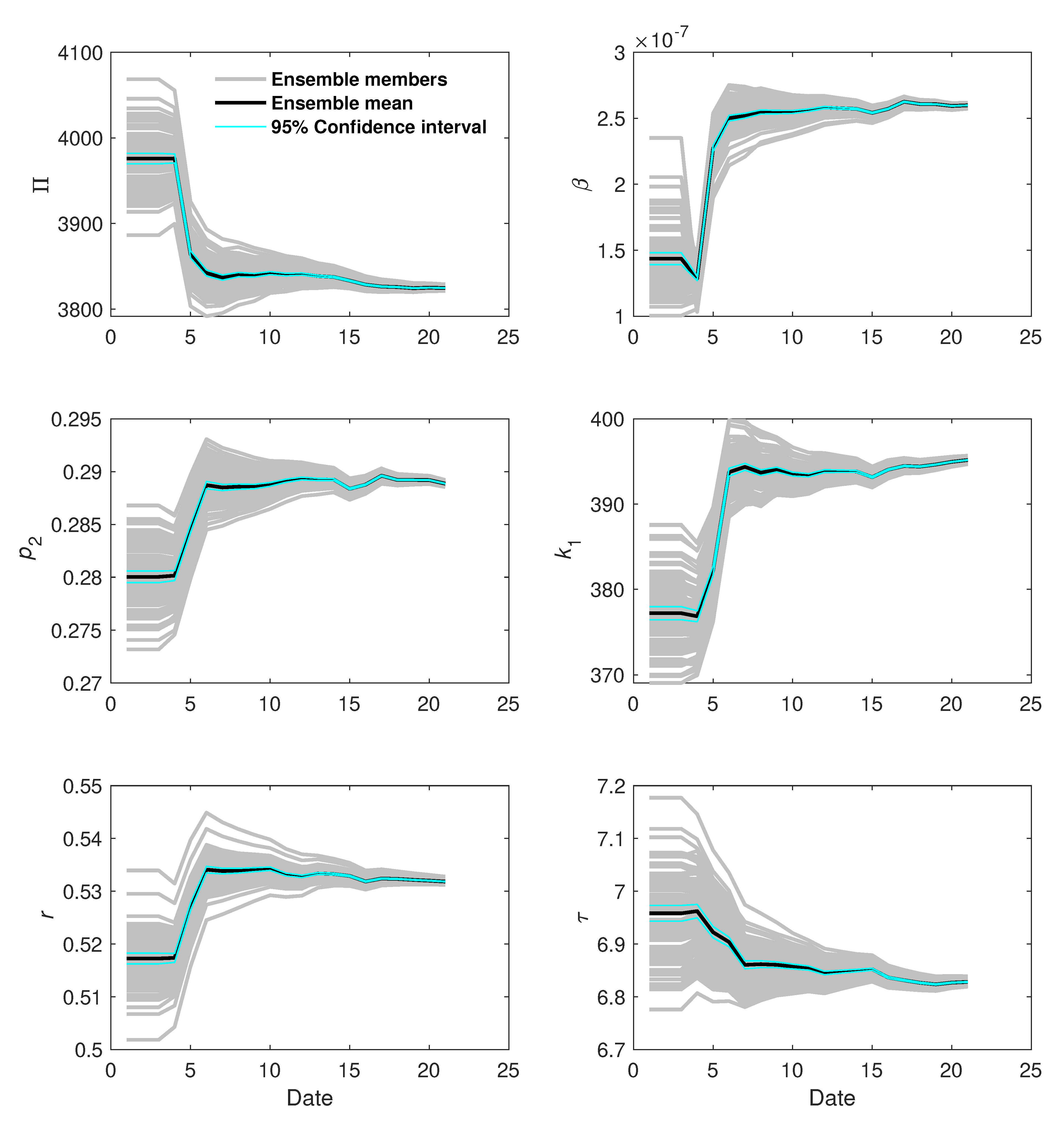
4.3. Assimilation Results

The time series of the viral load from the data, free-run (without data assimilation) and joint-EnKF run for all patients are shown in Figure 3. Compared to the model free-run, the joint-EnKF suggests significant improvements and yields more accurate viral load estimates. Although a few data points are not particularly well estimated by the joint-EnKF, the overall behavior of the viral load is well reproduced by the filter. To allow a quantifiable validation,

Table 2. Bias of the predicted viral load using the model free-run and the joint-EnKF and improvement (%) with respect to the model.

Patient	Model	Joint-EnKF	Improvement %
1	0.1496	0.0792	47.06
2	0.1646	0.1110	32.56
3	0.3566	0.1297	63.63
4	0.3131	0.2498	20.22
5	0.1853	0.1078	41.82
6	0.3255	0.1953	40.00

outlines the bias values comparing the measured and predicted viral load of the model free-run and the joint-EnKF for the six patients. The joint-EnKF results are also presented in terms of percentage improvement with respect to the model free-run prediction. The significantly improved filter estimates demonstrate the relevance of the data assimilation of the viral load information into the immune response model.

Closer examination of the results suggests that the viral load measurements for Patient 1 WEre very well predicted by the joint-EnKF. In particular, the viral load peak and the duration of high viral load WEre well captured. The joint-EnKF provides lower RAE compared to the model free-run, with an improvement reaching up to $50\%$. The model underestimates the peak level and does not accurately predict the rest of the hydrograph. For patients 2, 4 and 5, the viral load was satisfactory predicted by both the joint-EnKF and the model free-run, although the later fails to reproduce the peak level at the end of the Patient 5 hydrograph. The joint-EnKF further improves the prediction of the viral load for those patients by approximately $33\%$, $20\%$ and $42\%$, respectively. Both the joint-EnKF and the model free-run overestimate the peak level for Patient 3. While the joint-EnKF accurately predicts the rest of the hydrograph, the model free-run still overestimates the duration of the high viral load. The joint-EnKF is able to improve the viral load prediction by almost $63\%$. The same conclusion can be drawn for Patient 6, for whom the duration of the high viral load was overpredicted by the model free-run while the rest of the hydrograph is underestimated.

Overall, the performance of the model with and without data assimilation can be summarized as follows: (1) the peak level is well predicted almost everywhere by the filter, while it is occasionally overestimated or underestimated by the model free-run; (2) the model free-run solution is smooth compared to the joint- EnKF, which delineates the viral load dynamic much more accurately; and (3) the joint-EnKF is able to enhance the viral load estimation for all patients, improving the model solution by up to $40\%$ on average.

Figure 4 displays the time evolution of selected model parameters as estimated by the joint-EnKF for Patient 1. As seen, all parameters smoothly converge to a biologically acceptable range of values. The initial ensemble shrinks at each iteration showing a reduction of $95\%$ in the standard deviation at the end of the assimilation process. A similar assessment was made for the other parameters.

Table 3. Selected parameters and their converged values estimated by the joint-EnKF.

Patient	$\mathbf{\Pi }$	$\mathit{\beta }$	${\mathit{p}}_2$	${\mathit{k}}_1$	r	$\mathit{\tau }$
1	3824.63	$2.60\times {10}^{-7}$	0.2889	395.17	0.5318	6.83
2	3948.25	$3.26\times {10}^{-7}$	0.2943	376.06	0.5291	7.22
3	4036.26	$3.11\times {10}^{-7}$	0.2746	383.67	0.5157	9.52
4	3941.78	$1.43\times {10}^{-7}$	0.2840	369.57	0.5180	11.96
5	3916.61	$2.07\times {10}^{-7}$	0.2789	383.86	0.5190	7.43
6	3990.69	$1.54\times {10}^{-7}$	0.2835	372.31	0.5127	10.17

presents a summary of the selected parameters estimated by the joint-EnKF for all patients. The time delay for antibody production $\tau$ of patients 1, 2 and 5 was approximately 7 days and significantly lower than that for patients 3, 4 and 6 with values of $9.52$, $11.96$ and $10.17$ days, respectively. These results are quite consistent with the viral load hydrograph in Figure 3. As we can see, the viral load of patients 1, 2 and 5 start to decrease after almost 7 days. However, the decrease in the viral load for the other patients takes more time.

5. Conclusions

This paper formulated a nine-compartment mathematical model for simulating SARS-CoV-2 dynamics and the immune system response in infected patients. The model consists of healthy cells, infected cells, viral load, cytokines, natural killer cells, cytotoxic T-lymphocytes, B-lymphocytes, plasma cells and antibody levels. We computed the basic reproduction number and discussed the equilibrium states of the model. In order to reduce uncertainties in the model and improve its prediction skill, a joint state–parameter estimation scheme based on the EnKF was implemented. The joint-EnKF uses current viral load observations and applies a Kalman-based update to the dynamic state variables and parameters. Finally, we demonstrated the efficiency of the proposed methodology with real SARS-CoV-2 viral load data for six patients, while comparing its performance with the model free-run (i.e., without assimilation).

Sensitivity experiments using different ensemble sizes with the EnKF suggested that 100 members are sufficient to obtain reliable estimates with reasonable computational cost. During assimilation, the parameters’ ensembles were constrained by the data where the spread was reduced and eventually converged to a biologically acceptable range of values. In addition, the proposed joint-EnKF was able to reproduce the overall evolution of the dynamic process of the viral load evolution, the peak values, and the duration of the high viral load with significantly better accuracy than the model free-run. We also performed a quantitative analysis using the RAE comparing the measured and predicted viral load, and reported the percentage of improvements achieved by the joint-EnKF. The joint-EnKF consistently achieved better results for all patients, leading to an approximately $40\%$ improvement over the model free-run. This study demonstrated the relevance of the proposed assimilation system for enhancing the estimates of the immune response mathematical model.

References

1. Guan, W.J.; Ni, Z.Y.; Hu, Y.; Liang, W.H.; Ou, C.Q.; He, J.X.; Liu, L.; Shan, H.; Lei, C.l.; Hui, D.S.; et al. Clinical characteristics of coronavirus disease 2019 in China. N. Engl. J. Med. 2020, 382, 1708–1720. [Google Scholar] [CrossRef]
2. Sohrabi, C.; Alsafi, Z.; O’Neill, N.; Khan, M.; Kerwan, A.; Al-Jabir, A.; Iosifidis, C.; Agha, R. World Health Organization declares global emergency: A review of the 2019 novel coronavirus (COVID-19). Int. J. Surg. 2020, 76, 71–76. [Google Scholar] [CrossRef]
3. Brauer, F.; Castillo-Chavez, C.; Feng, Z. Mathematical Models in Epidemiology; Springer: Berlin/Heidelberg, Germany, 2019; Volume 32. [Google Scholar]
4. Choi, W.; Shim, E. Optimal strategies for vaccination and social distancing in a game-theoretic epidemiologic model. J. Theor. Biol. 2020, 505, 110422. [Google Scholar] [CrossRef] [PubMed]
5. Kumar, S.; Ahmadian, A.; Kumar, R.; Kumar, D.; Singh, J.; Baleanu, D.; Salimi, M. An efficient numerical method for fractional SIR epidemic model of infectious disease by using Bernstein wavelets. Mathematics 2020, 8, 558. [Google Scholar] [CrossRef] [Green Version]
6. Mahajan, A.; Sivadas, N.A.; Solanki, R. An epidemic model SIPHERD and its application for prediction of the spread of COVID-19 infection in India. Chaos Soliton Fractals 2020, 140, 110156. [Google Scholar] [CrossRef] [PubMed]
7. Ndaïrou, F.; Area, I.; Nieto, J.J.; Torres, D.F. Mathematical modeling of COVID-19 transmission dynamics with a case study of Wuhan. Chaos Soliton Fractals 2020, 135, 109846. [Google Scholar] [CrossRef] [PubMed]
8. Nkwayep, C.H.; Bowong, S.; Tewa, J.; Kurths, J. Short-term forecasts of the COVID-19 pandemic: Study case of Cameroon. Chaos Soliton Fractals 2020, 140, 110106. [Google Scholar] [CrossRef]
9. Saha, S.; Samanta, G. Modelling the role of optimal social distancing on disease prevalence of COVID-19 epidemic. Int. J. Dyn. Control 2020, 9, 1053–1077. [Google Scholar] [CrossRef]
10. Sarkar, K.; Khajanchi, S.; Nieto, J.J. Modeling and forecasting the COVID-19 pandemic in India. Chaos Soliton Fractals 2020, 139, 110049. [Google Scholar] [CrossRef]
11. Van Wees, J.D.; Osinga, S.; Van Der Kuip, M.; Tanck, M.W.; Tutu-van Furth, A. Forecasting hospitalization and ICU rates of the COVID-19 outbreak: An efficient SEIR model. Bull. World Health Organ. 2020. [Google Scholar] [CrossRef]
12. Yang, Q.; Yi, C.; Vajdi, A.; Cohnstaedt, L.W.; Wu, H.; Guo, X.; Scoglio, C.M. Short-term forecasts and long-term mitigation evaluations for the COVID-19 epidemic in Hubei Province, China. Infect. Dis. Model 2020, 5, 563–574. [Google Scholar]
13. Choi, W.; Shim, E. Optimal strategies for social distancing and testing to control COVID-19. J. Theor. Biol. 2021, 512, 110568. [Google Scholar] [CrossRef] [PubMed]
14. Ghostine, R.; Gharamti, M.; Hassrouny, S.; Hoteit, I. An extended SEIR model with vaccination for forecasting the COVID-19 pandemic in Saudi Arabia using an ensemble Kalman filter. Mathematics 2021, 9, 636. [Google Scholar] [CrossRef]
15. Du, S.Q.; Yuan, W. Mathematical modeling of interaction between innate and adaptive immune responses in COVID-19 and implications for viral pathogenesis. J. Med. Virol. 2020, 92, 1615–1628. [Google Scholar] [CrossRef] [PubMed]
16. Ghosh, I. Within host dynamics of SARS-CoV-2 in humans: Modeling immune responses and antiviral treatments. arXiv 2020, arXiv:2006.02936. [Google Scholar]
17. Hernandez-Vargas, E.A.; Velasco-Hernandez, J.X. In-host mathematical modelling of COVID-19 in humans. Annu. Rev. Control 2020, 50, 448–456. [Google Scholar] [CrossRef] [PubMed]
18. Chimal-Eguia, J.C. Mathematical Model of Antiviral Immune Response against the COVID-19 Virus. Mathematics 2021, 9, 1356. [Google Scholar] [CrossRef]
19. Edwards, C.A.; Moore, A.M.; Hoteit, I.; Cornuelle, B.D. Regional ocean data assimilation. Ann. Rev. Mar. Sci. 2015, 7, 21–42. [Google Scholar] [CrossRef] [Green Version]
20. Hoteit, I.; Luo, X.; Bocquet, M.; Kohl, A.; Ait-El-Fquih, B. Data assimilation in oceanography: Current status and new directions. New Front. Oper. Oceanogr. 2018, 2018, 465–512. [Google Scholar]
21. Hoteit, I.; Luo, X.; Pham, D.T. Particle Kalman filtering: A nonlinear Bayesian framework for ensemble Kalman filters. Mon. Weather Rev. 2012, 140, 528–542. [Google Scholar] [CrossRef] [Green Version]
22. Hoteit, I.; Pham, D.T.; Blum, J. A simplified reduced order Kalman filtering and application to altimetric data assimilation in Tropical Pacific. J. Mar. Syst. 2002, 36, 101–127. [Google Scholar] [CrossRef]
23. Hoteit, I.; Hoar, T.; Gopalakrishnan, G.; Collins, N.; Anderson, J.; Cornuelle, B.; Köhl, A.; Heimbach, P. A MITgcm/DART ensemble analysis and prediction system with application to the Gulf of Mexico. Dynam. Atmos. Ocean 2013, 63, 1–23. [Google Scholar] [CrossRef]
24. Buehner, M.; McTaggart-Cowan, R.; Heilliette, S. An ensemble Kalman filter for numerical weather prediction based on variational data assimilation: VarEnKF. Mon. Weather Rev. 2017, 145, 617–635. [Google Scholar] [CrossRef]
25. Gharamti, M.; Tjiputra, J.; Bethke, I.; Samuelsen, A.; Skjelvan, I.; Bentsen, M.; Bertino, L. Ensemble data assimilation for ocean biogeochemical state and parameter estimation at different sites. Ocean Model. 2017, 112, 65–89. [Google Scholar] [CrossRef]
26. Yu, L.; Fennel, K.; Bertino, L.; El Gharamti, M.; Thompson, K.R. Insights on multivariate updates of physical and biogeochemical ocean variables using an Ensemble Kalman Filter and an idealized model of upwelling. Ocean Model. 2018, 126, 13–28. [Google Scholar] [CrossRef]
27. Raboudi, N.F.; Ait-El-Fquih, B.; Dawson, C.; Hoteit, I. Combining Hybrid and One-Step-Ahead Smoothing for Efficient Short-Range Storm Surge Forecasting with an Ensemble Kalman Filter. Mon. Weather Rev. 2019, 147, 3283–3300. [Google Scholar] [CrossRef]
28. Gharamti, M.; Kadoura, A.; Valstar, J.; Sun, S.; Hoteit, I. Constraining a compositional flow model with flow-chemical data using an ensemble-based Kalman filter. Water Resour. Res. 2014, 50, 2444–2467. [Google Scholar] [CrossRef] [Green Version]
29. Gharamti, M.; Ait-El-Fquih, B.; Hoteit, I. An iterative ensemble Kalman filter with one-step-ahead smoothing for state-parameters estimation of contaminant transport models. J. Hydrol. 2015, 527, 442–457. [Google Scholar] [CrossRef] [Green Version]
30. Ait-El-Fquih, B.; Gharamti, M.E.; Hoteit, I. A Bayesian consistent dual ensemble Kalman filter for state-parameter estimation in subsurface hydrology. Hydrol. Earth Syst. Sci. 2016, 20, 3289–3307. [Google Scholar] [CrossRef] [Green Version]
31. Khaki, M.; Ait-El-Fquih, B.; Hoteit, I. Calibrating land hydrological models and enhancing their forecasting skills using an ensemble Kalman filter with one-step-ahead smoothing. J. Hydrol. 2020, 584, 124708. [Google Scholar] [CrossRef]
32. Kimura, N.; Hsu, M.H.; Tsai, M.Y.; Tsao, M.C.; Yu, S.L.; Tai, A. A river flash flood forecasting model coupled with ensemble Kalman filter. J. Flood Risk Manag. 2016, 9, 178–192. [Google Scholar] [CrossRef]
33. Ziliani, M.G.; Ghostine, R.; Ait-El-Fquih, B.; McCabe, M.F.; Hoteit, I. Enhanced flood forecasting through ensemble data assimilation and joint state-parameter estimation. J. Hydrol. 2019, 577, 123924. [Google Scholar] [CrossRef]
34. Kalman, R.E. A new approach to linear filtering and prediction problems. J. Mar. Syst. 1960, 82, 35–45. [Google Scholar] [CrossRef] [Green Version]
35. Evensen, G. The ensemble Kalman filter: Theoretical formulation and practical implementation. Ocean Dyn. 2003, 53, 343–367. [Google Scholar] [CrossRef]
36. Nikin-Beers, R.; Ciupe, S.M. The role of antibody in enhancing dengue virus infection. Math. Biosci. 2015, 263, 83–92. [Google Scholar] [CrossRef]
37. Duffin, R.P.; Tullis, R.H. Mathematical models of the complete course of HIV infection and AIDS. J. Theor. Biol. 2002, 4, 215–221. [Google Scholar] [CrossRef] [Green Version]
38. Clapham, H.E.; Tricou, V.; Van Vinh Chau, N.; Simmons, C.P.; Ferguson, N.M. Within-host viral dynamics of dengue serotype 1 infection. J. R. Soc. Interface 2014, 11, 20140094. [Google Scholar] [CrossRef] [PubMed] [Green Version]
39. Ben-Shachar, R.; Koelle, K. Minimal within-host dengue models highlight the specific roles of the immune response in primary and secondary dengue infections. J. R. Soc. Interface 2015, 12, 20140886. [Google Scholar] [CrossRef] [PubMed]
40. Sasmal, S.K.; Dong, Y.; Takeuchi, Y. Mathematical modeling on T-cell mediated adaptive immunity in primary dengue infections. J. Theor. Biol. 2017, 429, 229–240. [Google Scholar] [CrossRef] [PubMed]
41. Gujarati, T.P.; Ambika, G. Virus antibody dynamics in primary and secondary dengue infections. J. Math. Biol. 2014, 69, 1773–1800. [Google Scholar] [CrossRef] [PubMed] [Green Version]
42. Van den Driessche, P.; Watmough, J. Reproduction numbers and sub-threshold endemic equilibria for compartmental models of disease transmission. Math. Biosci. 2002, 180, 29–48. [Google Scholar] [CrossRef]
43. Martcheva, M. An Introduction to Mathematical Epidemiology; Springer: Berlin/Heidelberg, Germany, 2015; Volume 61. [Google Scholar]
44. Wölfel, R.; Corman, V.M.; Guggemos, W.; Seilmaier, M.; Zange, S.; Müller, M.A.; Niemeyer, D.; Jones, T.C.; Vollmar, P.; Rothe, C.; et al. Virological assessment of hospitalized patients with COVID-2019. Nature 2020, 581, 465–469. [Google Scholar] [CrossRef] [PubMed] [Green Version]
Figure 1. Schematic diagram of the proposed mathematical model. The cyan arrows indicate production, black arrows indicate activation, and orange arrows indicate attack.
Mathematics 09 02427 g001
Figure 2. RAE of the viral load for Patient 1 for different ensemble sizes.
Mathematics 09 02427 g002
Figure 3. Time series of the viral load for (a) Patient 1; (b) Patient 2; (c) Patient 3; (d) Patient 4; (e) Patient 5; and (f) Patient 6—relative to the model free-run (without assimilation), joint-EnKF, and the real data [44].
Mathematics 09 02427 g003
Figure 4. Time evolution of selected parameters estimated by the joint-EnKF for Patient 1.
Mathematics 09 02427 g004