On the First-Passage Time Problem for a Feller-Type Diffusion Process

Abstract

We consider the first-passage time problem for the Feller-type diffusion process, having infinitesimal drift $B_1(x,t)=\alpha \left(t\right)x+\beta \left(t\right)$ and infinitesimal variance $B_2(x,t)=2r\left(t\right)x$, defined in the space state $[0,+\infty )$, with $\alpha \left(t\right)\in \mathbb{R}$, $\beta \left(t\right)>0$, $r\left(t\right)>0$ continuous functions. For the time-homogeneous case, some relations between the first-passage time densities of the Feller process and of the Wiener and the Ornstein–Uhlenbeck processes are discussed. The asymptotic behavior of the first-passage time density through a time-dependent boundary is analyzed for an asymptotically constant boundary and for an asymptotically periodic boundary. Furthermore, when $\beta \left(t\right)=\xi r\left(t\right)$, with $\xi >0$, we discuss the asymptotic behavior of the first-passage density and we obtain some closed-form results for special time-varying boundaries.

1. Introduction

Diffusion processes are often used to describe the development of dynamic systems in a broad variety of scientific disciplines, including physics, biology, population dynamics, neurology, finance, and queueing. There is much interest in analyzing the “first-passage time” (FPT) issue in various situations. This entails determining the probability distribution of a random variable that describes the moment at which a process, beginning from a fixed initial state, reaches a defined boundary or threshold for the first time, which may also be time-varying. Unfortunately, closed-form solutions for the FPT densities are only accessible in a limited number of instances, leaving the more difficult job of determining the FPT densities through time-dependent boundaries.

Some general methods to solve FPT problems are based on:

• Analytical methods to determine the Laplace transform of FPT probability density function (pdf) and its moments for time-homogeneous diffusion process and constant boundaries (cf., for instance, Darling and Siegert [1], Blake and Lindsey [2], Giorno et al. [3]);
• Symmetry properties of transition density to obtain closed-form results on the FPT densities through time-dependent boundaries and other related functions (cf., for instance, Di Crescenzo et al. [4]);
• Construction of FPT pdf by making use of certain transformations among diffusion processes (cf., for instance, Gutiérrez et al. [5], Di Crescenzo et al. [6], Giorno and Nobile [7]);
• Formulation of integral equations for the FPT density (cf., for instance, Buonocore et al. [8], Gutiérrez et al. [9], Di Nardo et al [10]);
• Analysis of the asymptotic behavior of FPT pdf for large boundary or large times (cf., for instance, Nobile et al. [11,12])
• Efficient numerical algorithms and simulation procedures to estimate FPT pdf’s (cf., for instance, Herrmann and Zucca [13], Giraudo et al. [14], Taillefumier and Magnasco [15], Giorno and Nobile [16], Naouara and Trabelsi [17]).

In the present paper, we focus on the FPT problem for the Feller-type diffusion process.

Let $\{X\left(t\right),t\ge t_0\}$, $t_0\ge 0$, be a time-inhomogeneous Feller-type diffusion process, defined in the state space $[0,+\infty )$, which satisfies the following stochastic differential equation:

$$dX\left(t\right)=[\alpha \left(t\right)X\left(t\right)+\beta \left(t\right)]dt+\sqrt{2r\left(t\right)X\left(t\right)}dW\left(t\right),X\left(t_0\right)=x_0,$$

where $W\left(t\right)$ is a standard Wiener process. Hence, the infinitesimal drift and infinitesimal variance of $X\left(t\right)$ are

$$B_1(x,t)=\alpha \left(t\right)x+\beta \left(t\right),B_2(x,t)=2r\left(t\right)x$$

(1)

and we assume that $\alpha \left(t\right)\in \mathbb{R}$, $\beta \left(t\right)>0$, $r\left(t\right)>0$ are continuous functions for all $t\ge t_0$.

The Feller diffusion process plays a relevant role in different fields: in mathematical biology to model the growth of a population (cf. Feller [18], Lavigne and Roques [19], Masoliver [20], Pugliese and Milner [21]), in queueing systems to describe the number of customers in a queue (cf. Di Crescenzo and Nobile [22]), in neurobiology to analyze the input–output behavior of single neurons (see, for instance, Giorno et al. [23], Buonocore et al. [24], Ditlevsen and Lánský [25], Lánský et al. [26], Nobile and Pirozzi [27], D’Onofrio et al. [28]), in mathematical finance to model interest rates and stochastic volatility (see Cox et al. [29], Tian and Zhang [30], Maghsoodi [31], Peng and Schellhorn [32]). In population dynamics, the Feller-type diffusion process arises as a continuous approximation of a linear birth–death process with immigration (cf., for instance, Giorno and Nobile [33]). The Feller process has the advantage of having a state space bounded from below, a property that in the neuronal models allows the inclusion of the effect of reversal hyperpolarization potential. In this context, the statistical estimation of parameters of the Feller process starting from observations of its first-passage times plays a relevant role (cf., for instance, Ditlevsen and Lánský [25], Ditlevsen and Ditlevsen [34]). The study of the Feller process is also interesting in chemical reaction dynamics (cf., for instance, [35]).

For the Feller-type diffusion process $X\left(t\right)$, we assume that the total probability mass is conserved in $(0,+\infty )$ and we denote by $f(x,t|x_0,t_0)=\partial P\{X\left(t\right)\le x|X\left(t_0\right)=x_0\}/\partial x$ the transition pdf of $X\left(t\right)$ in the presence of a zero-flux condition in the zero state (cf., for instance, Giorno and Nobile [33]). Moreover, for the process $X\left(t\right)$, we consider the random variable

$$\mathcal{T}(x_0,t_0)=\left\{\begin{array}{c}\underset{t\ge t_0}{inf}\{t:X\left(t\right)\ge S\left(t\right)\},X\left(t_0\right)=x_0<S\left(t_0\right),\hfill \\ \hfill \\ \underset{t\ge t_0}{inf}\{t:X\left(t\right)\le S\left(t\right)\},X\left(t_0\right)=x_0>S\left(t_0\right),\hfill \end{array}\right.$$

(2)

which denotes the FPT of $X\left(t\right)$ from $X\left(t_0\right)=x_0$ to the continuous boundary $S\left(t\right)$. The FPT pdf $g[S\left(t\right),t|x_0,t_0]=\partial P(\mathcal{T}(x_0,t_0)\le t)/\partial t$ satisfies the first-kind Volterra integral equation (cf., for instance, Fortet [36]):

$$\begin{array}{ccc}& & f(x,t|x_0,t_0)={\int }_{t_0}^{t}g[S\left(u\right),u|x_0,t_0]f[x,t|S\left(u\right),u]du\hfill \\ & & [x_0<S\left(t_0\right),x\ge S\left(t\right)]\mathrm{or}[x_0>S\left(t_0\right),x\le S\left(t\right)].\hfill \end{array}$$

(3)

The renewal Equation (3) expresses that any sample path that reaches $x\ge S\left(t\right)$$[x\le S(t\left)\right]$, after starting from $x_0<S\left(t_0\right)$$[x_0>S\left(t_0\right)]$ at time $t_0$, must necessarily cross $S\left(u\right)$ for the first time at some intermediate instant $u\in (t_0,t)$. Research on the FPT problem for the Feller diffusion process has been carried out by Giorno et al. [37], Linetsky [38], Masoliver and Perelló [39], Masoliver [40], Chou and Lin [41], Di Nardo and D’Onofrio [42], Giorno and Nobile [43]).

The paper is structured as follows. In Section 2, we consider the time-homogeneous Feller process with a zero-flux condition in the zero state. For this process, we analyze the FPT problem through a constant boundary S starting from the initial state $x_0$ by determining the Laplace transform of the FPT density and the ultimate FPT probability in the following cases: (a) $x_0>S\ge 0$ and (b) $0\le x_0<S$. In particular, a closed-form expression for the FPT pdf through the zero state is given. Moreover, some connections between the FPT densities of the Feller process and the Wiener and Ornstein–Uhlenbeck processes are investigated. In Section 3, making use of the iterative Siegert formula, the first three FPT moments are obtained and analyzed. In Section 4, we study the asymptotic behavior of the FPT density when the time-varying boundary $S\left(t\right)$ moves away from the starting point $x_0$ for large time by distinguishing two cases: $S\left(t\right)$ is an asymptotically constant boundary and $S\left(t\right)$ is an asymptotically periodic boundary.

Section 5 is dedicated to the time-inhomogeneous Feller process in the proportional case. Specifically, we assume that $\alpha \left(t\right)$ is a real function, $r\left(t\right)>0$ and $\beta \left(t\right)=\xi r\left(t\right)$, with $\xi >0$. For this case, we determine the closed-form expression of the FPT density through the zero state. Furthermore, for $\xi =1/2$ and $\xi =3/2$, we obtain the FPT density through a specific time-varying boundary and the related ultimate FPT probability. Finally, in Section 6, an asymptotic exponential approximation is derived for asymptotically constant boundaries.

Various numerical computations are performed both for the time-homogeneous Feller process and for the time-inhomogeneous Feller-type process to analyze the role of the parameters.

2. FPT Problem for a Time-Homogeneous Feller Process

We consider the time-homogeneous Feller process $X\left(t\right)$ with drift $B_1\left(x\right)=\alpha x+\beta$ and infinitesimal variance $B_2\left(x\right)=2rx$, defined in the state space $[0,+\infty )$. As proved by Feller [44], the state $x=0$ is an exit boundary for $\beta \le 0$, a regular boundary for $0<\beta <r$ and an entrance boundary for $\beta \ge r$. The scale function and the speed density of $X\left(t\right)$ are (cf. Karlin and Taylor [45]):

$$\begin{array}{cc}\hfill & h\left(x\right)=exp\left\{-2{\int }^x\frac{B_1\left(z\right)}{B_2\left(z\right)}dz\right\}=x^{-\beta /r}exp\left\{-\frac{\alpha x}{r}\right\},\hfill \\ \hfill & s\left(x\right)=\frac{2}{B_2\left(x\right)h\left(x\right)}=\frac{x^{\beta /r-1}}{r}exp\left\{\frac{\alpha x}{r}\right\},\hfill \end{array}$$

(4)

respectively. In this section, we assume that $\beta >0$ and suppose that a zero-flux condition is placed in the zero state.

2.1. Transition Density

When $\alpha \in \mathbb{R}$, $\beta >0$ and $r>0$, imposing a zero-flux condition in the zero state, the transition pdf of $X\left(t\right)$ can be explicitly obtained (cf., for instance, Giorno et al. [37], Sacerdote [46]). Indeed, when $\alpha =0$, $\beta >0$ and $r>0$, the transition pdf is:

$$f(x,t|x_0,t_0)=\left\{\begin{array}{cc}\frac{1}{x\Gamma (\beta /r)}{\left[\frac{x}{r(t-t_0)}\right]}^{\beta /r}exp\left\{-\frac{x}{r(t-t_0)}\right\},\hfill & x_0=0,\hfill \\ \\ \frac{1}{r(t-t_0)}{\left(\frac{x}{x_0}\right)}^{(\beta -r)/\left(2r\right)}exp\left\{-\frac{x_0+x}{r(t-t_0)}\right\}\hfill \\ \times I_{\beta /r-1}\left[\frac{2\sqrt{x{x}_0}}{r(t-t_0)}\right],\hfill & x_0>0,\hfill \end{array}\right.$$

(5)

whereas if $\alpha \ne 0$, $\beta >0$ and $r>0$, one obtains:

$$f(x,t|x_0,t_0)=\left\{\begin{array}{cc}\frac{1}{x\Gamma (\beta /r)}{\left[\frac{\alpha x}{r(e^{\alpha (t-t_0)}-1)}\right]}^{\beta /r}exp\left\{-\frac{\alpha x}{r(e^{\alpha (t-t_0)}-1)}\right\},\hfill & x_0=0,\hfill \\ \\ \frac{\alpha }{r(e^{\alpha (t-t_0)}-1)}{\left[\frac{x{e}^{-\alpha (t-t_0)}}{x_0}\right]}^{(\beta -r)/\left(2r\right)}exp\left\{-\frac{\alpha [x+x_0{e}^{\alpha (t-t_0)}]}{r(e^{\alpha (t-t_0)}-1)}\right\}\hfill \\ \times I_{\beta /r-1}\left[\frac{2\alpha \sqrt{x{x}_0{e}^{\alpha (t-t_0)}}}{r(e^{\alpha (t-t_0)}-1)}\right],\hfill & x_0>0,\hfill \end{array}\right.$$

(6)

where

$$I_{\nu }\left(z\right)=\sum _{k=0}^{+\infty }\frac{1}{k!\Gamma (\nu +k+1)}{\left(\frac{z}{2}\right)}^{2k+\nu },\nu \in \mathbb{R}$$

(7)

denotes the modified Bessel function of the first kind and $\Gamma \left(\xi \right)$ is Eulero’s gamma function. Here and elsewhere, whenever the multiple-valued functions such as ${\left(\frac{z}{2}\right)}^{2k+\nu }$ appear, they are assumed to be taken as their principal branches. We note that the transition pdf $f(x,t|x_0,t_0)$ in (5) and (6) satisfies the following relation:

$$f(x,t|x_0,t_0)={\left(\frac{x}{x_0}\right)}^{\beta /r-1}exp\left\{\frac{\alpha (x-x_0)}{r}\right\}f(x_0,t|x,t_0),x_0>0,x>0.$$

(8)

Moreover, when $\alpha <0$, $\beta >0$ and $r>0$, the time-homogeneous Feller process allows a steady-state density:

$$W\left(x\right)=\underset{t\to +\infty }{lim}f(x,t|x_0,t_0)=\frac{1}{x\Gamma (\beta /r)}{\left(\frac{\left|\alpha \right|x}{r}\right)}^{\beta /r}exp\left\{-\frac{\left|\alpha \right|x}{r}\right\},x>0,$$

(9)

which is a gamma density of parameters $\beta /r$ and $r/\left|\alpha \right|$. In the sequel, we denote by

$$q_{\lambda }\left(x\right|x_0)={\int }_0^{+\infty }{e}^{-\lambda t}q(x,t|x_0)dt,\lambda >0$$

the Laplace transform (LT) of the function $q(x,t|x_0)\equiv q(x,t|x_0,0)$.

2.2. Laplace Transform of the Transition Density

By performing the LT to (5) and (6), for $0\le x_0<x$ one has (cf. Giorno et al. [37], Chou and Lin [41]):

$$f_{\lambda }\left(x\right|x_0)=\left\{\begin{array}{cc}\frac{e^{-\left|\alpha \right|x/r}{x}^{\beta /r-1}}{\left|\alpha \right|\Gamma \left(\beta /r\right)}{\left(\frac{\left|\alpha \right|}{r}\right)}^{\beta /r}\Gamma \left(\frac{\lambda }{\left|\alpha \right|}\right)\Psi \left(\frac{\lambda }{\left|\alpha \right|},\frac{\beta }{r};\frac{\left|\alpha \right|x}{r}\right)\Phi \left(\frac{\lambda }{\left|\alpha \right|},\frac{\beta }{r};\frac{\left|\alpha \right|x_0}{r}\right),\hfill & \alpha <0,\hfill \\ \\ \frac{2}{r}{\left(\frac{x}{x_0}\right)}^{\beta /\left(2r\right)-1/2}{K}_{\beta /r-1}\left(2\sqrt{\frac{\lambda x}{r}}\right)I_{\beta /r-1}\left(2\sqrt{\frac{\lambda x_0}{r}}\right),\hfill & \alpha =0,\hfill \\ \\ \frac{e^{-\alpha x_0/r}{x}^{\beta /r-1}}{\alpha \Gamma \left(\beta /r\right)}{\left(\frac{\alpha }{r}\right)}^{\beta /r}\Gamma \left(\frac{\lambda }{\alpha }+\frac{\beta }{r}\right)\Psi \left(\frac{\lambda }{\alpha }+\frac{\beta }{r},\frac{\beta }{r};\frac{\alpha x}{r}\right)\Phi \left(\frac{\lambda }{\alpha }+\frac{\beta }{r},\frac{\beta }{r};\frac{\alpha x_0}{r}\right),\hfill & \alpha >0,\hfill \end{array}\right.$$

(10)

where

$$K_{\nu }\left(x\right)=\frac{\pi }{2}\frac{I_{-\nu }\left(x\right)-I_{\nu }\left(x\right)}{sin\left(\nu \pi \right)},$$

(11)

denotes the modified Bessel function of the second kind (cf. Gradshteyn and Ryzhik [47], p. 928, no. 8.485) and

$$\begin{array}{cc}\hfill & \Phi (a,c;x)=1+\sum _{n=1}^{+\infty }\frac{{\left(a\right)}_n}{{\left(c\right)}_n}\frac{x^n}{n!},\hfill \\ \hfill & \Psi (a,c;x)=\frac{\Gamma (1-c)}{\Gamma (a-c+1)}\Phi (a,c;x)+\frac{\Gamma (c-1)}{\Gamma \left(a\right)}{x}^{1-c}\Phi (a-c+1,2-c;x),\hfill \end{array}$$

(12)

are the Kummer’s functions of the first and second kinds, respectively (cf. Gradshteyn and Ryzhik [47], p. 1023, no. 9.210.1 and no. 9.210.2). Kummer’s functions satisfy the following relations (cf. Tricomi [48]):

$$\Phi (a,c;x)=e^x\Phi (c-a,c;-x),\Phi (a,a;x)=e^x$$

(13)

and

$$\Psi (a,c;x)=x^{1-c}\Psi (a-c+1,2-c;x),\Psi (0,c;x)=1,\Psi (c,c;x)=e^x\Gamma (1-c,x),$$

(14)

where

$$\Gamma (a,x)={\int }_x^{+\infty }{e}^{-t}{t}^{a-1}dt$$

(15)

denotes the incomplete gamma function. By performing the Laplace transform to both sides of (8), the following result is obtained:

$$f_{\lambda }\left(x\right|x_0)={\left(\frac{x}{x_0}\right)}^{\beta /r-1}exp\left\{\frac{\alpha (x-x_0)}{r}\right\}{f}_{\lambda }\left(x_0\right|x),x_0>0,x>0.$$

(16)

2.3. Laplace Transform of the FPT Density

An analytic approach to analyze the FPT problem through a non-negative constant boundary $S\left(t\right)=S$ is based on the Laplace transform. Indeed, from (3), one has:

$$g_{\lambda }\left(x\right|x_0)=\frac{f_{\lambda }\left(x\right|x_0)}{f_{\lambda }\left(x\right|S)},[x_0<S\le x]\mathrm{or}[x\le S<x_0],$$

(17)

so that the LT of the FPT pdf $g(S,t|x_0)$ can be evaluated by knowing the LT of the transition pdf $f(S,t|x_0)$.

To determine $g_{\lambda }\left(S\right|x_0)$ via (17), we consider the following cases: (a) $x_0>S\ge 0$ and (b) $0\le x_0<S$.

(a)

FPT downwards for the time-homogeneous Feller process

For $x_0>S>0$, by virtue of (16) and (17), one has:

$$g_{\lambda }\left(S\right|x_0)=\frac{f_{\lambda }\left(S\right|x_0)}{f_{\lambda }\left(S\right|S)}={\left(\frac{S}{x_0}\right)}^{\beta /r-1}exp\left\{\frac{\alpha (S-x_0)}{r}\right\}\frac{f_{\lambda }\left(x_0\right|S)}{f_{\lambda }\left(S\right|S)}·$$

(18)

Then, making use of (10) in (18), for $x_0>S>0$, one obtains:

$$g_{\lambda }\left(S\right|x_0)=\left\{\begin{array}{cc}\frac{\Psi \left(\frac{\lambda }{\left|\alpha \right|},\frac{\beta }{r};\frac{\left|\alpha \right|x_0}{r}\right)}{\Psi \left(\frac{\lambda }{\left|\alpha \right|},\frac{\beta }{r};\frac{\left|\alpha \right|S}{r}\right)},\hfill & \alpha <0,\hfill \\ {\left(\frac{S}{x_0}\right)}^{\beta /\left(2r\right)-1/2}\frac{K_{\beta /r-1}\left(2\sqrt{\frac{\lambda x_0}{r}}\right)}{K_{\beta /r-1}\left(2\sqrt{\frac{\lambda S}{r}}\right)},\hfill & \alpha =0,\hfill \\ exp\left\{\frac{\alpha (S-x_0)}{r}\right\}\frac{\Psi \left(\frac{\lambda }{\alpha }+\frac{\beta }{r},\frac{\beta }{r};\frac{\alpha x_0}{r}\right)}{\Psi \left(\frac{\lambda }{\alpha }+\frac{\beta }{r},\frac{\beta }{r};\frac{\alpha S}{r}\right)},\hfill & \alpha >0.\hfill \end{array}\right.$$

(19)

From (19), one derives the ultimate FPT probability through S starting from $x_0$, with $x_0>S>0$:

$$P\left(S\right|x_0)={\int }_0^{+\infty }g(S,t|x_0)dt=\left\{\begin{array}{cc}1,\hfill & [\alpha <0,\beta >0]\mathrm{or}[\alpha =0,0<\beta \le r],\hfill \\ {\left(\frac{S}{x_0}\right)}^{\beta /r-1},\hfill & \alpha =0,\beta >r,\hfill \\ \frac{\Gamma \left(1-\frac{\beta }{r},\frac{\alpha x_0}{r}\right)}{\Gamma \left(1-\frac{\beta }{r},\frac{\alpha S}{r}\right)},\hfill & \alpha >0,\beta >0,\hfill \end{array}\right.$$

(20)

with the use of (11) and (14). Furthermore, if $x_0>0$, taking the limit as $S\downarrow 0$ in (19), for $0<\beta <r$, one has:

$$g_{\lambda }\left(0\right|x_0)=\left\{\begin{array}{cc}\frac{\Gamma \left(1-\frac{\beta }{r}+\frac{\lambda }{\left|\alpha \right|}\right)}{\Gamma \left(1-\frac{\beta }{r}\right)}\Psi \left(\frac{\lambda }{\left|\alpha \right|},\frac{\beta }{r};\frac{\left|\alpha \right|x_0}{r}\right),\hfill & \alpha <0,\hfill \\ \frac{2}{\Gamma \left(1-\frac{\beta }{r}\right)}{\left(\frac{\lambda x_0}{r}\right)}^{1/2-\beta /\left(2r\right)}{K}_{\beta /r-1}\left(2\sqrt{\frac{\lambda x_0}{r}}\right),\hfill & \alpha =0,\hfill \\ exp\left\{-\frac{\alpha x_0}{r}\right\}\frac{\Gamma \left(1+\frac{\lambda }{\alpha }\right)}{\Gamma \left(1-\frac{\beta }{r}\right)}\Psi \left(\frac{\lambda }{\alpha }+\frac{\beta }{r},\frac{\beta }{r};\frac{\alpha x_0}{r}\right),\hfill & \alpha >0,\hfill \end{array}\right.$$

(21)

where the relation

$$\Psi (a,c;0)=\frac{\Gamma (1-c)}{\Gamma (a-c+1)},0<Rec<1,$$

has been used for $\alpha \ne 0$, whereas the identity

$$\Gamma \left(a\right)\Gamma (1-a)=\frac{\pi }{sin\left(a\pi \right)}0<a<1.$$

has been applied for $\alpha =0$. From (21), one obtains the ultimate FPT probability through zero state starting from $x_0$, with $x_0>0$:

$$P\left(0\right|x_0)={\int }_0^{+\infty }g(0,t|x_0)dt=\left\{\begin{array}{cc}1,\hfill & \alpha \le 0,0<\beta <r,\hfill \\ 1-\frac{\gamma \left(1-\frac{\beta }{r},\frac{\alpha x_0}{r}\right)}{\Gamma \left(1-\frac{\beta }{r}\right)},\hfill & \alpha >0,0<\beta <r,\hfill \end{array}\right.$$

(22)

where

$$\gamma (a,x)={\int }_0^x{t}^{a-1}{e}^{-t}dt=\Gamma \left(a\right)-\Gamma (a,x),Rea>0,$$

denotes the incomplete gamma function.

For $x_0>0$ and $0<\beta <r$, the inverse LT of $g_{\lambda }\left(0\right|x_0)$, given in (21), can be explicitly evaluated:

$$g(0,t|x_0,t_0)=\left\{\begin{array}{cc}\frac{1}{(t-t_0)\Gamma \left(1-\frac{\beta }{r}\right)}{\left(\frac{x_0}{r(t-t_0)}\right)}^{1-\beta /r}exp\left\{-\frac{x_0}{r(t-t_0)}\right\},\hfill & \alpha =0,\hfill \\ \frac{1}{\Gamma \left(1-\frac{\beta }{r}\right)}\frac{\alpha }{e^{\alpha (t-t_0)}-1}{\left[\frac{\alpha x_0{e}^{\alpha (t-t_0)}}{r(e^{\alpha (t-t_0)}-1)}\right]}^{1-\beta /r}exp\left\{-\frac{\alpha x_0{e}^{\alpha (t-t_0)}}{r(e^{\alpha (t-t_0)}-1)}\right\},\hfill & \alpha \ne 0.\hfill \end{array}\right.$$

(23)

Indeed, since (cf. Erdelyi et al. [49], p. 283, no. 35)

$${\lambda }^{-\nu /2}{K}_{\nu }\left(2\sqrt{a\lambda }\right)=\frac{a^{-\nu /2}}{2}{\int }_0^{+\infty }{e}^{-\lambda t}{t}^{\nu -1}{e}^{-a/t}dt,a>0,$$

the start of (23) follows from (21) for $\alpha =0$. Moreover, for $\alpha \ne 0$ making use of the first of (14) in (21) and recalling that (cf. Tricomi [48], p. 90)

$$\Psi (s,c;z)=\frac{1}{\Gamma \left(s\right)}{\int }_0^{+\infty }{e}^{-s\tau }exp\left\{-\frac{z}{e^{\tau }-1}\right\}{(1-e^{-\tau })}^{-c}d\tau ,Rez>0,Res>0,$$

the second part of (23) is obtained.

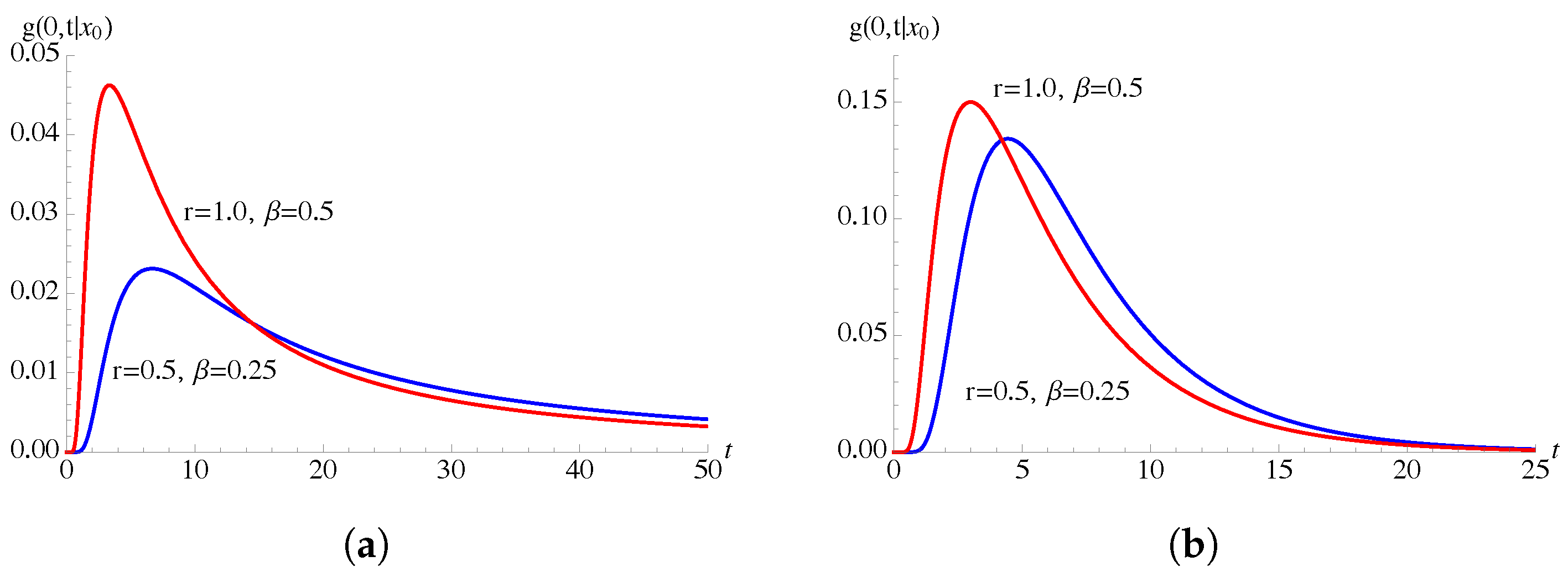
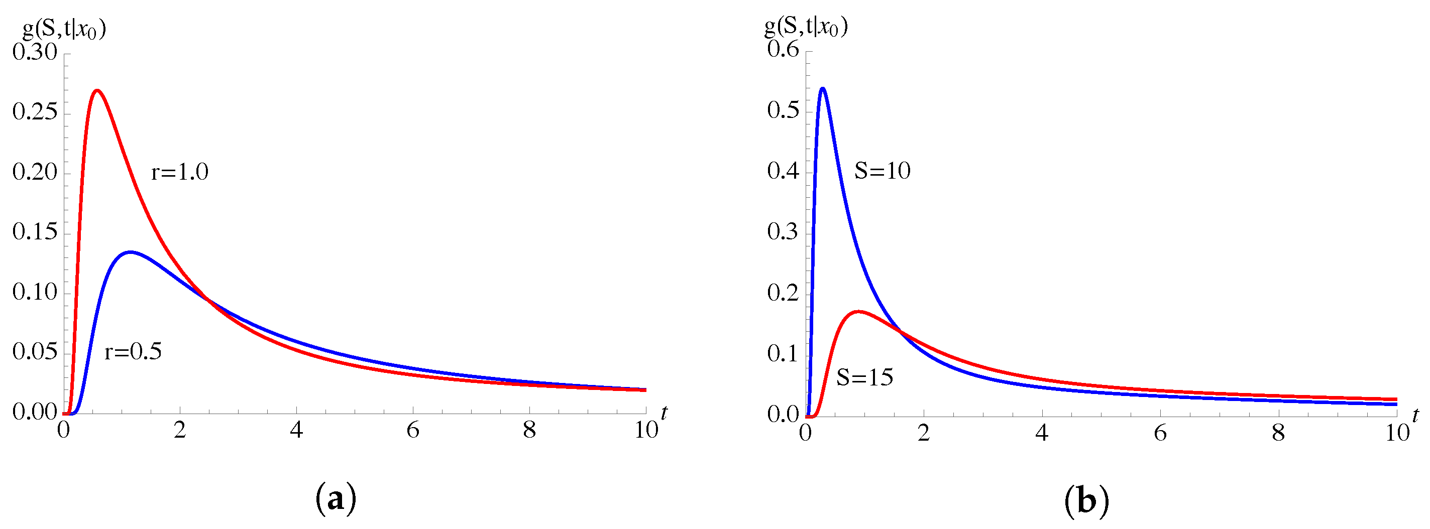
In Figure 1, the FPT pdf $g(0,t|x_0,t_0)$, given in (23), is plotted as function of t for some choices of $\alpha$ and r, with $\beta =r/2$.

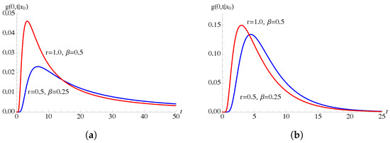
Figure 1. The FPT pdf (23) is plotted as function of t for t₀ = 0, x₀ = 5. (a) FPT pdf for α = 0. (b) FPT pdf for α = −0.5.

(b)

FPT upwards for the time-homogeneous Feller process

By virtue of (10), from (17), for $0<x_0<S$, one has

$$g_{\lambda }\left(S\right|x_0)=\frac{f_{\lambda }\left(S\right|x_0)}{f_{\lambda }\left(S\right|S)}=\left\{\begin{array}{cc}\frac{\Phi \left(\frac{\lambda }{\left|\alpha \right|},\frac{\beta }{r};\frac{\left|\alpha \right|x_0}{r}\right)}{\Phi \left(\frac{\lambda }{\left|\alpha \right|},\frac{\beta }{r};\frac{\left|\alpha \right|S}{r}\right)},\hfill & \alpha <0,\hfill \\ {\left(\frac{S}{x_0}\right)}^{\beta /\left(2r\right)-1/2}\frac{I_{\beta /r-1}\left(2\sqrt{\frac{\lambda x_0}{r}}\right)}{I_{\beta /r-1}\left(2\sqrt{\frac{\lambda S}{r}}\right)},\hfill & \alpha =0,\hfill \\ exp\left\{\frac{\alpha (S-x_0)}{r}\right\}\frac{\Phi \left(\frac{\lambda }{\alpha }+\frac{\beta }{r},\frac{\beta }{r};\frac{\alpha x_0}{r}\right)}{\Phi \left(\frac{\lambda }{\alpha }+\frac{\beta }{r},\frac{\beta }{r};\frac{\alpha S}{r}\right)},\hfill & \alpha >0,\hfill \end{array}\right.$$

(24)

whereas for $x_0=0$ and $S>0$, it results that:

$$g_{\lambda }\left(S\right|0)=\frac{f_{\lambda }\left(S\right|0)}{f_{\lambda }\left(S\right|S)}=\left\{\begin{array}{cc}\frac{1}{\Phi \left(\frac{\lambda }{\left|\alpha \right|},\frac{\beta }{r};\frac{\left|\alpha \right|S}{r}\right)},\hfill & \alpha <0,\hfill \\ \frac{1}{\Gamma \left(\frac{\beta }{r}\right)}{\left(\frac{\lambda S}{r}\right)}^{\beta /\left(2r\right)-1/2}\frac{1}{I_{\beta /r-1}\left(2\sqrt{\frac{\lambda S}{r}}\right)},\hfill & \alpha =0,\hfill \\ exp\left\{\frac{\alpha S}{r}\right\}\frac{1}{\Phi \left(\frac{\lambda }{\alpha }+\frac{\beta }{r},\frac{\beta }{r};\frac{\alpha S}{r}\right)},\hfill & \alpha >0.\hfill \end{array}\right.$$

(25)

From (24) and (25), one derives that the first passage through S starting from $x_0$ is a sure event, i.e.,

$$P\left(S\right|x_0)={\int }_0^{+\infty }g(S,t|x_0)dt=1,0\le x_0<S.$$

(26)

2.4. Relations between the FPT Densities for the Feller and the Wiener Processes

The FPT pdf $g(S,t|x_0,t_0)$ for the time-homogeneous Feller process can be explicitly obtained for $\alpha =0$ and $\beta =r/2$ or for $\alpha =0$ and $\beta =3r/2$, as proved in Proposition 1 and in Proposition 2, respectively. Moreover, in these cases, there is a relationship between the FPT pdf of Feller process and the FPT pdf of the standard Wiener process.

Proposition 1.

Let $X\left(t\right)$ be a time-homogeneous Feller diffusion process, having $B_1\left(x\right)=r/2$ and $B_2\left(x\right)=2rx$, with a zero-flux condition in the zero state.

• If $x_0>S\ge 0$, one has:

  $$g(S,t|x_0,t_0)=\frac{\sqrt{x_0}-\sqrt{S}}{\sqrt{\pi r{(t-t_0)}^3}}exp\left\{-\frac{{(\sqrt{x_0}-\sqrt{S})}^2}{r(t-t_0)}\right\}$$

  (27)
  and $P\left(S\right|x_0)=1$.
• If $0\le x_0<S$, one obtains:

  $$\begin{array}{ccc}& & g(S,t|x_0,t_0)=\frac{\sqrt{S}-\sqrt{x_0}}{\sqrt{\pi r{(t-t_0)}^3}}exp\left\{-\frac{{(\sqrt{S}-\sqrt{x_0})}^2}{r(t-t_0)}\right\}\hfill \\ & & \times \{1+2\sum _{j=1}^{+\infty }{(-1)}^{j}exp\left\{-\frac{4j^{2}S}{r(t-t_0)}\right\}[cosh\left(\frac{4j\sqrt{S}(\sqrt{S}-\sqrt{x_0})}{r(t-t_0)}\right)\hfill \\ & & -\frac{2j\sqrt{S}}{\sqrt{S}-\sqrt{x_0}}sinh\left(\frac{4j\sqrt{S}(\sqrt{S}-\sqrt{x_0})}{r(t-t_0)}\right)\left]\right\},\hfill \end{array}$$

  (28)
  or alternatively

  $$\begin{array}{ccc}& & g(S,t|x_0,t_0)=\frac{\pi r}{4S}\sum _{n=1}^{+\infty }{(-1)}^{n-1}(2n-1)exp\left\{-\frac{{(2n-1)}^2{\pi }^{2}r(t-t_0)}{16S}\right\}\hfill \\ & & \times cos\left[\frac{(2n-1)\pi }{2}\sqrt{\frac{x_0}{S}}\right],\hfill \end{array}$$

  (29)
  and $P\left(S\right|x_0)=1$.

Proof. 

We assume that $\alpha =0$ and $\beta =r/2$. In this case, the zero state is a regular reflecting boundary. Making use of the relations (cf. Abramowitz and Stegun [50], p. 443, no. 10.2.14 and p. 444, no. 10.2.17)

$$I_{-1/2}\left(x\right)=\sqrt{\frac{2}{\pi }}\frac{cosh\left(x\right)}{\sqrt{x}},K_{-1/2}\left(x\right)=\sqrt{\frac{\pi }{2x}}{e}^{-x},$$

from (19), (21), (24) and (25) with $\alpha =0$ and $\beta =r/2$, it follows that:

$$g_{\lambda }\left(S\right|x_0)=\left\{\begin{array}{cc}exp\left\{-\sqrt{2\lambda }\left(\sqrt{\frac{2x_0}{r}}-\sqrt{\frac{2S}{r}}\right)\right\},\hfill & x_0>S\ge 0,\hfill \\ \frac{cosh\left(2\sqrt{\frac{\lambda x_0}{r}}\right)}{cosh\left(2\sqrt{\frac{\lambda S}{r}}\right)},\hfill & 0\le x_0<S.\hfill \end{array}\right.$$

(30)

When $x_0>S\ge 0$, the right-hand side of (30) identifies with the LT $g_{\lambda }^{\left(W\right)}\left(\sqrt{2S/r}\right|\sqrt{2x_0/r})$ of the FPT pdf $g_W$ through $\sqrt{2S/r}$ for a standard Wiener process originated in $\sqrt{2x_0/r}$. Hence, for $\alpha =0$ and $\beta =r/2$, one has

$$g(S,t|x_0,t_0)=g_W\left(\sqrt{\frac{2S}{r}},t|\sqrt{\frac{2x_0}{r}},t_0\right),x_0>S\ge 0,$$

from which (27) follows. Instead, for $0\le x_0<S$, the right-hand side of (30) is the LT ${\gamma }_{\lambda }^{\left(W\right)}\left(\sqrt{2S/r}\right|\sqrt{2x_0/r})$ of the FPT pdf ${\gamma }_W$ through $\sqrt{2S/r}$ for a standard Wiener process, starting from $\sqrt{2x_0/r}$, restricted to $[0,+\infty )$ with 0 reflecting boundary (cf., for instance, Giorno and Nobile [3]). Then, for $\alpha =0$ and $\beta =r/2$, one obtains:

$$g(S,t|x_0,t_0)={\gamma }_W\left(\sqrt{\frac{2S}{r}},t|\sqrt{\frac{2x_0}{r}},t_0\right),0\le x_0<S,$$

from which (28) follows. The alternative expression (29) is derived by performing the inverse LT to the second expression in (30) and by using formula 33.149, p. 190 in Spiegel et al.’s work [51]. □

We note that by setting $S=0$ in (27) we obtain (23) with $\alpha =0$ and $\beta =r/2$.

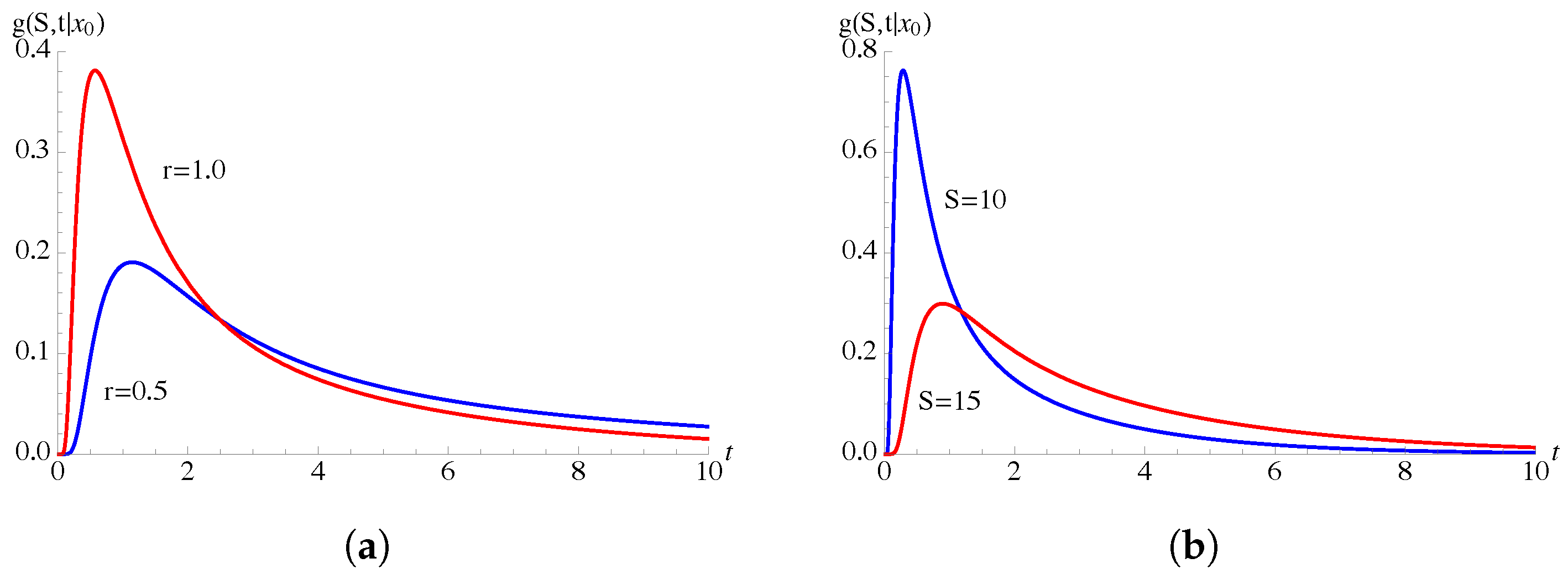
In Figure 2, the FPT pdf (28) is plotted as function of t for $t_0=0$, $x_0=5$ and various choices of parameters r and S.

Figure 2. The FPT pdf (28) is plotted as function of t for t₀ = 0 and x₀ = 5. (a) FPT pdf for S = 10. (b) FPT pdf for r = 2.

Proposition 2.

Let $X\left(t\right)$ be a time-homogeneous Feller diffusion process, having $B_1\left(x\right)=3r/2$ and $B_2\left(x\right)=2rx$, with a zero-flux condition in the zero state.

• If $x_0>S>0$, one has:

  $$g(S,t|x_0,t_0)=\sqrt{\frac{S}{x_0}}\frac{\sqrt{x_0}-\sqrt{S}}{\sqrt{\pi r{(t-t_0)}^3}}exp\left\{-\frac{{(\sqrt{x_0}-\sqrt{S})}^2}{r(t-t_0)}\right\}$$

  (31)
  and $P\left(S\right|x_0)=\sqrt{S/x_0}$.
• If $0<x_0<S$, one obtains:

  $$\begin{array}{ccc}& & g(S,t|x_0,t_0)=\sqrt{\frac{S}{x_0}}\frac{\sqrt{S}-\sqrt{x_0}}{\sqrt{\pi r{(t-t_0)}^3}}exp\left\{-\frac{{(\sqrt{S}-\sqrt{x_0})}^2}{r(t-t_0)}\right\}\hfill \\ & & \times \{1+2\sum _{j=1}^{+\infty }exp\left\{-\frac{4j^{2}S}{r(t-t_0)}\right\}[cosh\left(\frac{4j\sqrt{S}(\sqrt{S}-\sqrt{x_0})}{r(t-t_0)}\right)\hfill \\ & & -\frac{2j\sqrt{S}}{\sqrt{S}-\sqrt{x_0}}sinh\left(\frac{4j\sqrt{S}(\sqrt{S}-\sqrt{x_0})}{r(t-t_0)}\right)\left]\right\},\hfill \end{array}$$

  (32)
  or alternatively

  $$g(S,t|x_0,t_0)=\frac{\pi r}{2\sqrt{x_{0}S}}\sum _{n=1}^{+\infty }{(-1)}^{n+1}nexp\left\{-\frac{n^2{\pi }^{2}r(t-t_0)}{4S}\right\}sin\left(n\pi \sqrt{\frac{x_0}{S}}\right),$$

  (33)
  and $P\left(S\right|x_0)=1$.
• If $x_0=0$ and $S>0$, one has:

  $$\begin{array}{ccc}& & g(S,t|0,t_0)=\frac{4\sqrt{S}}{\sqrt{\pi r{(t-t_0)}^3}}exp\left\{-\frac{S}{r(t-t_0)}\right\}\sum _{j=1}^{+\infty }jexp\left\{-\frac{4j^{2}S}{r(t-t_0)}\right\}\hfill \\ & & \times \left[\frac{4jS}{r(t-t_0)}cosh\left(\frac{4jS}{r(t-t_0)}\right)-\left(1+\frac{2S}{r(t-t_0)}\right)sinh\left(\frac{4jS}{r(t-t_0)}\right)\right],\hfill \end{array}$$

  (34)
  or alternatively

  $$g(S,t|0,t_0)=\frac{{\pi }^{2}r}{2S}\sum _{n=1}^{+\infty }{(-1)}^{n+1}{n}^{2}exp\left\{-\frac{n^2{\pi }^{2}r(t-t_0)}{4S}\right\},$$

  (35)
  and $P\left(S\right|x_0)=1$.

Proof. 

We assume that $\alpha =0$ and $\beta =3r/2$. In this case, the zero state is an entrance boundary. Making use of the relations (cf. Abramowitz and Stegun [50], p. 443, no. 10.2.13 and p. 444, no. 10.2.17)

$$I_{1/2}\left(x\right)=\sqrt{\frac{2}{\pi }}\frac{sinh\left(x\right)}{\sqrt{x}},K_{1/2}\left(x\right)=\sqrt{\frac{\pi }{2x}}{e}^{-x},$$

from (19), (24) and (25) with $\alpha =0$ and $\beta =3r/2$, it follows that:

$$g_{\lambda }\left(S\right|x_0)=\left\{\begin{array}{cc}\sqrt{\frac{S}{x_0}}exp\left\{-\sqrt{2\lambda }\left(\sqrt{\frac{2x_0}{r}}-\sqrt{\frac{2S}{r}}\right)\right\},\hfill & x_0>S>0,\hfill \\ \sqrt{\frac{S}{x_0}}\frac{sinh\left(2\sqrt{\frac{\lambda x_0}{r}}\right)}{sinh\left(2\sqrt{\frac{\lambda S}{r}}\right)},\hfill & 0<x_0<S,\hfill \\ 2\sqrt{\frac{\lambda S}{r}}\frac{1}{sinh\left(2\sqrt{\frac{\lambda S}{r}}\right)},\hfill & x_0=0,S>0.\hfill \end{array}\right.$$

(36)

We note that when $x_0>S>0$, the right-hand side of (36) identifies with the LT $\sqrt{S/x_0}{g}_{\lambda }^{\left(W\right)}\left(\sqrt{2S/r}\right|\sqrt{2x_0/r})$ of the function $\sqrt{S/x_0}{g}_W$, where $g_W$ is the FPT pdf through $\sqrt{2S/r}$ of a standard Wiener process originated in $\sqrt{2x_0/r}$. Hence, for $\alpha =0$ and $\beta =3r/2$, one has

$$g(S,t|x_0,t_0)=\sqrt{\frac{S}{x_0}}{g}_W\left(\sqrt{\frac{2S}{r}},t|\sqrt{\frac{2x_0}{r}},t_0\right),x_0>S>0,$$

that leads to (32). Instead, for $0<x_0<S$ the right-hand side of (36) is the LT $\sqrt{S/x_0}{h}_{\lambda }^{\left(W\right)}\left(\sqrt{2S/r}\right|\sqrt{2x_0/r})$ of the function $\sqrt{S/x_0}{h}_W$, where $h_W$ is the first-exit time pdf through $\sqrt{2S/r}$ for a standard Wiener process, starting from $\sqrt{2x_0/r}$, defined in $(0,+\infty )$ with 0 absorbing boundary (cf., for instance, Giorno and Nobile [3]). Then, for $\alpha =0$ and $\beta =3r/2$, one has

$$g(S,t|x_0,t_0)=\sqrt{\frac{S}{x_0}}{h}_W\left(\sqrt{\frac{2S}{r}},t|\sqrt{\frac{2x_0}{r}},t_0\right),0<x_0<S,$$

from which (32) follows. The alternative expression (33) can be obtained by performing the inverse LT to the second expression in (36) and by using formula 33.148, p. 190 in Spiegel et al. [51] (by changing the sign). Finally, (34) and (35) follow by taking the limit as $x_0\downarrow 0$ in (32) and (33), respectively. □

In Figure 3, the FPT pdf (32) is plotted as function of t for $t_0=0$, $x_0=5$ and various choices of parameters r and S. We note that, due to the different nature of the zero state, the peaks of FPT densities of Figure 3 are more pronounced with respect to those of Figure 2.

Figure 3. The FPT pdf (32) is plotted as function of t for t₀ = 0, x₀ = 5. (a) FPT pdf for S = 10. (b) FPT pdf for r = 2.

2.5. Relations between the FPT Densities for the Feller and the Ornstein–Uhlenbeck Processes

For $\alpha \ne 0$ and $\beta =r/2$ or $\alpha \ne 0$ and $\beta =3r/2$, the FPT pdf $g(S,t|x_0,t_0)$ of the Feller process can be related to the FPT pdf of the Ornstein–Uhlenbeck process.

Proposition 3.

Let $X\left(t\right)$ be a time-homogeneous Feller diffusion process, having $B_1\left(x\right)=\alpha x+r/2$ and $B_2\left(x\right)=2rx$ ($\alpha \ne 0$), with a zero-flux condition in the zero state.

• If $x_0>S\ge 0$, one has:

  $$g_{\lambda }\left(S\right|x_0)=\left\{\begin{array}{cc}exp\left\{\frac{\left|\alpha \right|(x_0-S)}{2r}\right\}\frac{D_{-2\lambda /\left|\alpha \right|}\left(\sqrt{\frac{2\left|\alpha \right|x_0}{r}}\right)}{D_{-2\lambda /\left|\alpha \right|}\left(\sqrt{\frac{2\left|\alpha \right|S}{r}}\right)},\hfill & \alpha <0,\hfill \\ exp\left\{-\frac{\alpha (x_0-S)}{2r}\right\}\frac{D_{-1-2\lambda /\alpha }\left(\sqrt{\frac{2\alpha x_0}{r}}\right)}{D_{-1-2\lambda /\alpha }\left(\sqrt{\frac{2\alpha S}{r}}\right)},\hfill & \alpha >0,\hfill \end{array}\right.$$

  (37)
  where $D_{\nu }\left(x\right)$ denotes the parabolic cylinder function, and

  $$P\left(S\right|x_0)=\left\{\begin{array}{cc}1,\hfill & \alpha <0,\hfill \\ \frac{1-\mathrm{Erf}\left(\sqrt{\frac{\alpha x_0}{r}}\right)}{1-\mathrm{Erf}\left(\sqrt{\frac{\alpha S}{r}}\right)},\hfill & \alpha >0,\hfill \end{array}\right.$$

  (38)
  where $\mathrm{Erf}\left(x\right)=(2/\sqrt{\pi }){\int }_0^{+\infty }{e}^{-z^2}dz$ denotes the error function.
• If $0\le x_0<S$, one obtains:

  $$g_{\lambda }\left(S\right|x_0)=\left\{\begin{array}{cc}\frac{\Phi \left(\frac{\lambda }{\left|\alpha \right|},\frac{1}{2};\frac{\left|\alpha \right|x_0}{r}\right)}{\Phi \left(\frac{\lambda }{\left|\alpha \right|},\frac{1}{2};\frac{\left|\alpha \right|S}{r}\right)},\hfill & \alpha <0,\hfill \\ exp\left\{\frac{\alpha (S-x_0)}{r}\right\}\frac{\Phi \left(\frac{\lambda }{\alpha }+\frac{1}{2},\frac{1}{2};\frac{\alpha x_0}{r}\right)}{\Phi \left(\frac{\lambda }{\alpha }+\frac{1}{2},\frac{1}{2};\frac{\alpha S}{r}\right)},\hfill & \alpha >0\hfill \end{array}\right.$$

  (39)
  and $P\left(S\right|x_0)=1$.

Proof. 

Let $\alpha \ne 0$ and $\beta =r/2$. We assume that the state $x=0$ is a regular reflecting boundary. Recalling that (cf. Tricomi [48], p. 219, no. (1)):

$$D_{\nu }\left(x\right)=2^{\nu /2}{e}^{-x^2/4}\Psi \left(-\frac{\nu }{2},\frac{1}{2};\frac{x^2}{2}\right),Rex>0,$$

(40)

for $x_0>S>0$ from (19) one obtains (37). Furthermore, for $x_0>0$ and $S=0$, from (21) with $\alpha \ne 0$ and $\beta =r/2$, making use of (40), we have

$$g_{\lambda }\left(0\right|x_0)=\left\{\begin{array}{cc}\frac{2^{\lambda /\left|\alpha \right|}}{\sqrt{\pi }}\Gamma \left(\frac{1}{2}+\frac{\lambda }{\left|\alpha \right|}\right)exp\left\{\frac{\left|\alpha \right|x_0}{2r}\right\}{D}_{-2\lambda /\left|\alpha \right|}\left(\sqrt{\frac{2\left|\alpha \right|x_0}{r}}\right),\hfill & \alpha <0,\hfill \\ \frac{2^{\lambda /\alpha +1/2}}{\sqrt{\pi }}\Gamma \left(1+\frac{\lambda }{\alpha }\right)exp\left\{-\frac{\alpha x_0}{2r}\right\}{D}_{-1-2\lambda /\alpha }\left(\sqrt{\frac{2\alpha x_0}{r}}\right),\hfill & \alpha >0.\hfill \end{array}\right.$$

(41)

Equation (41) identifies with (37) for $S=0$, being (cf. Tricomi [48], p. 221, no. (9)):

$$D_{\nu }\left(0\right)=\frac{\sqrt{\pi }{2}^{\nu /2}}{\Gamma \left(\frac{1-\nu }{2}\right)}·$$

(42)

Since (cf. Tricomi [48], p. 234, no. 15 and p. 235, no. 18):

$$D_0\left(x\right)=exp\left\{-\frac{x^2}{4}\right\},D_{-1}\left(x\right)=\sqrt{\frac{\pi }{2}}exp\left\{\frac{x^2}{4}\right\}\left[1-\mathrm{Erf}\left(\frac{x}{\sqrt{2}}\right)\right],$$

(43)

by setting $\lambda =0$ in (37), one obtains (38).

Instead, for $0\le x_0<S$, from (24) and (25), with $\alpha \ne 0$ and $\beta =r/2$, one immediately obtains (39). Consequently, by setting $\lambda =0$ and making use of the second expression in (13), it follows that $P\left(S\right|x_0)=1$. □

We note that, for $x_0>S\ge 0$, the right-hand side of (37) identifies with the LT $g_{\lambda }^{\left(\mathrm{OU}\right)}\left(\sqrt{2S/r}\right|\sqrt{2x_0/r})$ of the FPT pdf $g_{\mathrm{OU}}$ from $\sqrt{2x_0/r}$ through $\sqrt{2S/r}$ for the Ornstein–Uhlenbeck process with infinitesimal drift $C_1\left(x\right)=\alpha x/2$ and infinitesimal variance $C_2=1$. Hence, for $\alpha \ne 0$ and $\beta =r/2$ from (37) one has:

$$g(S,t|x_0,t_0)=g_{\mathrm{OU}}\left(\sqrt{\frac{2S}{r}},t|\sqrt{\frac{2x_0}{r}},t_0\right),x_0>S\ge 0.$$

(44)

Furthermore, for $0\le x_0<S$ the right-hand side of (39) is the LT ${\gamma }_{\lambda }^{\left(\mathrm{OU}\right)}\left(\sqrt{2S/r}\right|\sqrt{2x_0/r})$ of the FPT pdf ${\gamma }_{\mathrm{OU}}$ from $\sqrt{2x_0/r}$ to $\sqrt{2S/r}$ for the Ornstein–Uhlenbeck process with infinitesimal drift $C_1\left(x\right)=\alpha x/2$ and infinitesimal variance $C_2=1$, defined in $[0,+\infty )$, with 0 reflecting boundary. Therefore, for $\alpha \ne 0$ and $\beta =r/2$ from (39), one obtains:

$$g(S,t|x_0,t_0)={\gamma }_{\mathrm{OU}}\left(\sqrt{\frac{2S}{r}},t|\sqrt{\frac{2x_0}{r}},t_0\right),0\le x_0<S.$$

(45)

For $\alpha \ne 0$ and $\beta =r/2$, relations (44) and (45) show that the FPT density of the Feller process can be also interpreted as the the FPT density of an Ornstein–Uhlenbeck process, that is known only when $S=0$. Therefore, from (44), one has:

$$\begin{array}{ccc}& & g(0,t|x_0,t_0)=g_{\mathrm{OU}}\left(0,t|\sqrt{\frac{2x_0}{r}},t_0\right)\hfill \\ & & =\sqrt{\frac{x_0{e}^{\alpha (t-t_0)}}{r\pi }}{\left[\frac{\alpha }{e^{\alpha (t-t_0)}-1}\right]}^{3/2}exp\left\{-\frac{\alpha x_0{e}^{\alpha (t-t_0)}}{r(e^{\alpha (t-t_0)}-1)}\right\},x_0>0,\hfill \end{array}$$

which identifies with (23) for $\alpha \ne 0$ and $\beta =r/2$.

Proposition 4.

Let $X\left(t\right)$ be a time-homogeneous Feller diffusion process, having $B_1\left(x\right)=\alpha x+3r/2$ and $B_2\left(x\right)=2rx$ ($\alpha \ne 0$), with a zero-flux condition in the zero state.

• If $x_0>S>0$, one has:

  $$g_{\lambda }\left(S\right|x_0)=\left\{\begin{array}{cc}\sqrt{\frac{S}{x_0}}exp\left\{\frac{\left|\alpha \right|(x_0-S)}{2r}\right\}\frac{D_{1-2\lambda /\left|\alpha \right|}\left(\sqrt{\frac{2\left|\alpha \right|x_0}{r}}\right)}{D_{1-2\lambda /\left|\alpha \right|}\left(\sqrt{\frac{2\left|\alpha \right|S}{r}}\right)},\hfill & \alpha <0,\hfill \\ \sqrt{\frac{S}{x_0}}exp\left\{-\frac{\alpha (x_0-S)}{2r}\right\}\frac{D_{-2-2\lambda /\alpha }\left(\sqrt{\frac{2\alpha x_0}{r}}\right)}{D_{-2-2\lambda /\alpha }\left(\sqrt{\frac{2\alpha S}{r}}\right)},\hfill & \alpha >0\hfill \end{array}\right.$$

  (46)
  and

  $$P\left(S\right|x_0)=\left\{\begin{array}{cc}1,\hfill & \alpha <0,\hfill \\ \sqrt{\frac{S}{x_0}}\frac{1-\sqrt{\frac{\alpha x_0\pi }{r}}exp\left\{\frac{\alpha x_0}{r}\right\}[1-\mathrm{Erf}\left(\sqrt{\frac{\alpha x_0}{r}}\right)]}{1-\sqrt{\frac{\alpha S\pi }{r}}exp\left\{\frac{\alpha S}{r}\right\}[1-\mathrm{Erf}\left(\sqrt{\frac{\alpha S}{r}}\right)]},\hfill & \alpha >0.\hfill \end{array}\right.$$

  (47)
• If $0\le x_0<S$, one obtains:

  $$g_{\lambda }\left(S\right|x_0)=\left\{\begin{array}{cc}\frac{\Phi \left(\frac{\lambda }{\left|\alpha \right|},\frac{3}{2};\frac{\left|\alpha \right|x_0}{r}\right)}{\Phi \left(\frac{\lambda }{\left|\alpha \right|},\frac{3}{2};\frac{\left|\alpha \right|S}{r}\right)},\hfill & \alpha <0,\hfill \\ exp\left\{\frac{\alpha (S-x_0)}{r}\right\}\frac{\Phi \left(\frac{\lambda }{\alpha }+\frac{3}{2},\frac{3}{2};\frac{\alpha x_0}{r}\right)}{\Phi \left(\frac{\lambda }{\alpha }+\frac{3}{2},\frac{3}{2};\frac{\alpha S}{r}\right)},\hfill & \alpha >0\hfill \end{array}\right.$$

  (48)
  and $P\left(S\right|x_0)=1$.

Proof. 

Let $\alpha \ne 0$ and $\beta =3r/2$, so that the state $x=0$ is an entrance boundary. For $x_0>S>0$, recalling that (cf. Tricomi [48], p. 219, no. (2))

$$D_{\nu }\left(x\right)=2^{(\nu -1)/2}{e}^{-x^2/4}x\Psi \left(\frac{1-\nu }{2},\frac{3}{2};\frac{x^2}{2}\right),Rex>0,$$

(49)

from (19), with $\alpha \ne 0$ and $\beta =3r/2$, one obtains (46). Moreover, making use of relation $D_{\nu +1}\left(x\right)=x{D}_{\nu }\left(x\right)-\nu D_{\nu -1}\left(x\right)$ and of (43), one has

$$D_1\left(x\right)=xexp\left\{-\frac{x^2}{4}\right\},D_{-2}\left(x\right)=exp\left\{-\frac{x^2}{4}\right\}-\sqrt{\frac{\pi }{2}}xexp\left\{\frac{x^2}{4}\right\}\left[1-\mathrm{Erf}\left(\frac{x}{\sqrt{2}}\right)\right],$$

(50)

so that, by setting $\lambda =0$ in (46), one obtains (47).

Instead, for $0\le x_0<S$ from (24) and (25), with $\alpha \ne 0$ and $\beta =3r/2$, Equation (48) immediately follows. Finally, by setting $\lambda =0$ in (48) and making use of the second expression in (13), one has $P\left(S\right|x_0)=1$. □

For $x_0>S>0$, we note that the right-hand side of (46) identifies with the LT $\sqrt{S/x_0}{g}_{\lambda +\alpha /2}^{\left(\mathrm{OU}\right)}\left(\sqrt{2S/r}\right|\sqrt{2x_0/r})$ of $\sqrt{S/x_0}{e}^{-\alpha t/2}{g}_{\mathrm{OU}}$, where $g_{\mathrm{OU}}$ is the FPT pdf from $\sqrt{2x_0/r}$ through $\sqrt{2S/r}$ for the Ornstein–Uhlenbeck process with infinitesimal drift $C_1\left(x\right)=\alpha x/2$ and infinitesimal variance $C_2=1$. Hence, for $\alpha \ne 0$ and $\beta =3r/2$ one has:

$$g(S,t|x_0,t_0)=\sqrt{\frac{S}{x_0}}exp\{-\frac{\alpha (t-t_0)}{2}\}{g}_{\mathrm{OU}}\left(\sqrt{\frac{2S}{r}},t|\sqrt{\frac{2x_0}{r}},t_0\right),x_0>S>0.$$

(51)

For $\alpha \ne 0$ and $\beta =3r/2$, Equation (51) shows that a functional relationship between the FPT densities of the Feller and Ornstein–Uhlenbeck processes exists.

3. FPT Moments for the Time-Homogeneous Feller Process

When $P\left(S\right|x_0)=1$, the FPT moments of the time-homogeneous Feller process $X\left(t\right)$ with a zero-flux condition in the zero state

$$t_n\left(S\right|x_0)={\int }_0^{+\infty }{t}^{n}g(S,t|x_0)dt,n=1,2,\dots$$

can be evaluated via $g_{\lambda }\left(S\right|x_0)$ as:

$$t_n\left(S\right|x_0)={(-1)}^n\frac{d^n{g}_{\lambda }\left(S\right|x_0)}{d{\lambda }^n}{|}_{\lambda =0},n=1,2,\dots$$

We note that the computation of higher order derivatives becomes more and more laborious, making this procedure impractical for the Feller process. An alternative method is based on Siegert’s iterative formulas (cf. Siegert [52]) that hold for time-homogeneous diffusion processes. In particular, when $P\left(S\right|x_0)\equiv t_0\left(S\right|x_0)=1$, Siegert’s iterative formulas for the Feller process are the following:

• If $S<x_0$, then

  $$t_n\left(S\right|x_0)=n{\int }_S^{x_0}dzh\left(z\right){\int }_z^{+\infty }s\left(u\right)t_{n-1}\left(S\right|u)du,n=1,2,\dots .$$

  (52)
• If $S>x_0$, then

  $$t_n\left(S\right|x_0)=n{\int }_{x_0}^{S}dzh\left(z\right){\int }_0^{z}s\left(u\right)t_{n-1}\left(S\right|u)du,n=1,2,\dots$$

  (53)

  with $h\left(x\right)$ and $s\left(x\right)$ defined in (4).

3.1. Mean of FPT Downwards

We distinguish the cases $x_0>S>0$ and $x_0>0,S=0$.

If $x_0>S>0$ and $[\alpha <0,\beta >0]$ or $[\alpha =0,0<\beta \le r]$, we have proved in (20) that $P\left(S\right|x_0)=1$, so that from (52) for $\alpha =0$ and $0<\beta \le r$ one has that $t_1\left(S\right|x_0)$ diverges, whereas if $\alpha <0$ and $\beta >0$ one obtains:

$$\begin{array}{ccc}& & t_1\left(S\right|x_0)=\frac{1}{\left|\alpha \right|}\Gamma \left(\frac{\beta }{r}\right){\int }_{\left|\alpha \right|S/r}^{\left|\alpha \right|x_0/r}{z}^{-\beta /r}{e}^{z}dz-\frac{1}{\beta }\sum _{n=0}^{+\infty }\frac{1}{{(1+\beta /r)}_n}{\left(\frac{\left|\alpha \right|}{r}\right)}^n\frac{x_0^{n+1}-S^{n+1}}{n+1},\hfill \\ & & x_0>S>0.\hfill \end{array}$$

(54)

Moreover, for $x_0>0$ and $S=0$, due to (22), $P\left(0\right|x_0)=1$ if and only if $\alpha \le 0$ and $0<\beta <r$. Making use of (22), for $\alpha =0$ and $0<\beta <r$, one has that $t_1\left(0\right|x_0)$ diverges, whereas for $\alpha <0$ and $0<\beta <r$ the FPT mean is

$$\begin{array}{ccc}& & t_1\left(0\right|x_0)=\frac{1}{\left|\alpha \right|}\Gamma \left(\frac{\beta }{r}\right)\sum _{n=0}^{+\infty }\frac{1}{n!}\frac{1}{n+1-\beta /r}{\left(\frac{\left|\alpha \right|x_0}{r}\right)}^{n+1-\beta /r}\hfill \\ & & -\frac{1}{\beta }\sum _{n=0}^{+\infty }\frac{1}{{(1+\beta /r)}_n}{\left(\frac{\left|\alpha \right|}{r}\right)}^n\frac{x_0^{n+1}}{n+1},x_0>0.\hfill \end{array}$$

(55)

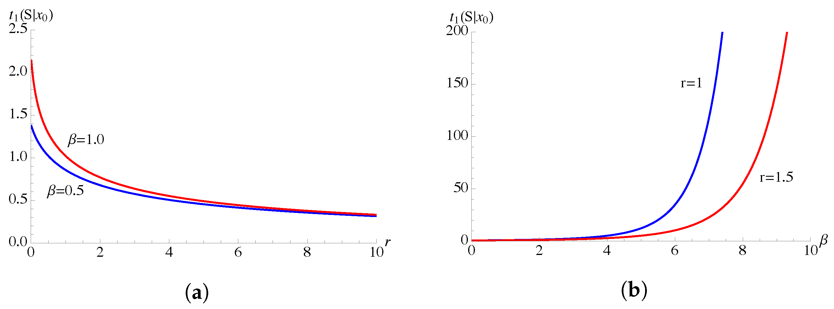
In Figure 4, the FPT mean (54) is plotted for $x_0=5$, $S=3$ and $\alpha =-0.5$ for different choices of $\beta$ and r. We note that $t_1\left(S\right|x_0)$ decreases as r increases, whereas it increases with $\beta$.

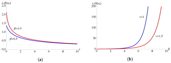
Figure 4. The FPT mean (54) is plotted for x₀ = 5, S = 3 and α = −0.5. (a) FPT mean as function of r. (b) FPT mean as function of β.

3.2. Moments of FPT Upwards

If $0\le x_0<S$, we have proved in (26) that $P\left(S\right|x_0)=1$, so that from (53) one has:

$$\begin{array}{cc}\hfill & t_1\left(S\right|x_0)=\frac{1}{\beta }\sum _{n=0}^{+\infty }\frac{1}{{(1+\beta /r)}_n}{\left(-\frac{\alpha }{r}\right)}^n\frac{S^{n+1}-x_0^{n+1}}{n+1},\hfill \\ \hfill & t_2\left(S\right|x_0)=\frac{2}{\beta }{t}_1\left(S\right|x_0)\sum _{n=0}^{+\infty }\frac{1}{{(1+\beta /r)}_n}{\left(-\frac{\alpha }{r}\right)}^n\frac{S^{n+1}}{n+1}\hfill \\ \hfill & -\frac{2r}{\beta }\sum _{n=1}^{+\infty }\frac{1}{{(1+\beta /r)}_n}{\left(-\frac{\alpha }{r}\right)}^{n+1}\frac{S^{n+1}-x_0^{n+1}}{n+1}\sum _{i=1}^n\frac{1}{i},\hfill \\ \hfill & t_3\left(S\right|x_0)=\frac{3}{\beta }{t}_2\left(S\right|x_0)\sum _{n=0}^{+\infty }\frac{1}{{(1+\beta /r)}_n}{\left(-\frac{\alpha }{r}\right)}^n\frac{S^{n+1}}{n+1}\hfill \\ \hfill & -\frac{6r}{\beta }{t}_1\left(S\right|x_0)\sum _{n=1}^{+\infty }\frac{1}{{(1+\beta /r)}_n}{\left(-\frac{\alpha }{r}\right)}^{n+1}\frac{S^{n+1}}{n+1}\sum _{i=1}^n\frac{1}{i}\hfill \\ \hfill & -\frac{6r}{\beta }\sum _{n=2}^{+\infty }\frac{1}{{(1+\beta /r)}_{n+2}}{\left(-\frac{\alpha }{r}\right)}^{n+1}\frac{S^{n+1}-x_0^{n+1}}{n+1}\sum _{i=2}^n\frac{1}{i}\sum _{j=2}^i\frac{1}{j-1}.\hfill \end{array}$$

(56)

In particular, when $\alpha <0$, from (56) it follows that:

• $t_1\left(S\right|x_0)$ decreases as r increases and ${lim}_{r\to +\infty }{t}_1\left(S\right|x_0)=(S-x_0)/\beta$;
• $t_1\left(S\right|x_0)$ decreases as $\beta$ increases and ${lim}_{\beta \to +\infty }{t}_1\left(S\right|x_0)=0$.

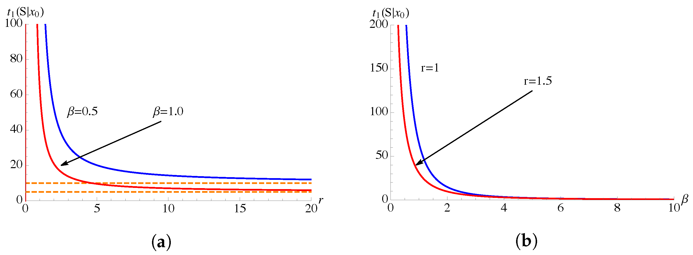
In Figure 5, the FPT mean (54) is plotted for $x_0=5$, $S=10$ and $\alpha =-0.5$ for several choices of $\beta$ and r.

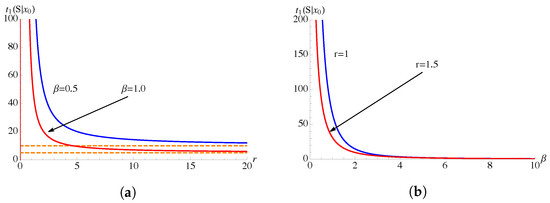
Figure 5. The FPT mean (54) is plotted for x₀ = 5, S = 10 and α = −0.5. (a) FPT mean as function of r, the dashed lines indicate the asymptotic limit (S − x₀)/β. (b) FPT mean as function of β.

The expressions (56) of the FPT moments are very complicated and do not allow us to highlight the quantitative behavior of the moments as a function of the involved parameters. Nevertheless, some unexpected features can be discovered as a result of systematic computations in which the mean $t_1\left(S\right|x_0)$, the variance $\mathrm{Var}\left(S\right|x_0)=t_2\left(S\right|x_0)-t_1^2\left(S\right|x_0)$, the coefficient of variation $\mathrm{Cv}\left(S\right|x_0)=\sqrt{\mathrm{Var}\left(S\right|x_0)}/t_1\left(S\right|x_0)$ and the skewness

$$\Sigma \left(S\right|x_0)=\frac{t_3\left(S\right|x_0)-3t_1\left(S\right|x_0)t_2\left(S\right|x_0)+2t_1^3\left(S\right|x_0)}{{\left[\mathrm{Var}\left(S\right|x_0)\right]}^{3/2}}$$

of the FPT are evaluated. In Table 1, $t_1\left(S\right|x_0)$$\mathrm{Var}\left(S\right|x_0)$, $\mathrm{Cv}\left(S\right|x_0)$ and $\Sigma \left(S\right|x_0)$ are listed for various boundaries and initial states, with $\alpha =-0.5$, $\beta =0.2$ and $r=1$. As shown in Table 1, for large boundaries the coefficient of variation of FPT approaches the value 1 and the skewness of the FPT approaches the value 2. Hence, when $\alpha <0$, it is argued that the FPT pdf of the Feller process is susceptible to an exponential approximation for a wide range of constant boundaries S and of initial states $x_0$, with $S>x_0$. This property does not occur when $\alpha \ge 0$. Table 1 also shows that the values of $t_1\left(S\right|x_0)$ and $\mathrm{Var}\left(S\right|x_0)$ become insensitive to the starting point $x_0$ of the process as the boundary S increases.

Table 1. For the Feller process, with $B_1\left(x\right)=-0.5x+0.2$ and $B_2\left(x\right)=2x$, the mean, the variance, the coefficient of variation and the skewness of FPT are listed for $x_0=0,5,10$ and for increasing values of the boundary $S>x_0$.

	S	${\mathit{t}}_1\left(\mathit{S}\right|\mathit{x}0)$	$\mathbf{Var}\left(\mathit{S}\right|{\mathit{x}}_0)$	$\mathbf{Cv}\left(\mathit{S}\right|\mathit{x}0)$	$\mathbf{\Sigma }\left(\mathit{S}\right|{\mathit{x}}_0)$
$x_0=0$	5	$9.111607\times {10}^1$	$7.918037\times {10}^3$	$0.976593$	$1.999485$
	10	$1.030455\times {10}^3$	$1.054126\times {10}^6$	0996362	$1.999973$
	20	$1.305581\times {10}^5$	$1.704399\times {10}^{10}$	$0.999958$	$1.998950$
	30	$1.771815\times {10}^7$	$3.139316\times {10}^{14}$	$0.999998$	$1.999116$
	40	$2.472975\times {10}^9$	$6.115604\times {10}^{18}$	$1.000000$	$1.998936$
	50	$3.502187\times {10}^{11}$	$1.226522\times {10}^{23}$	$0.999996$	$2.037217$
	60	$5.004295\times {10}^{13}$	$2.504289\times {10}^{27}$	$0.999998$	$2.002647$
	70	$7.194172\times {10}^{15}$	$5.175608\times {10}^{31}$	$1.000000$	$1.999006$
$x_0=5$	10	$9.393392\times {10}^2$	$1.046208\times {10}^6$	$1.088896$	$2.021401$
	20	$1.304670\times {10}^5$	$1.704398\times {10}^{10}$	$1.000656$	$1.999551$
	30	$1.771805\times {10}^7$	$3.139325\times {10}^{14}$	$1.000005$	$1.998926$
	40	$2.472975\times {10}^9$	$6.115603\times {10}^{18}$	$1.000000$	$1.997063$
	50	$3.502187\times {10}^{11}$	$1.226531\times {10}^{23}$	$1.000000$	$2.036733$
	60	$5.004295\times {10}^{13}$	$2.504283\times {10}^{27}$	$0.999997$	$2.002072$
	70	$7.194173\times {10}^{15}$	$5.175608\times {10}^{31}$	$1.000000$	$2.000006$
$x_0=10$	15	$1.041999\times {10}^4$	$1.299491\times {10}^8$	$1.094005$	$2.022940$
	20	$1.295276\times {10}^5$	$1.704293\times {10}^{10}$	$1.007882$	$1.999778$
	30	$1.771711\times {10}^7$	$3.139304\times {10}^{14}$	$1.000055$	$1.998418$
	40	$2.472974\times {10}^9$	$6.115604\times {10}^{18}$	$1.000000$	$1.999088$
	50	$3.502187\times {10}^{11}$	$1.226532\times {10}^{23}$	$1.000000$	$1.981817$
	60	$5.004295\times {10}^{13}$	$2.504274\times {10}^{27}$	$0.999995$	$2.002118$
	70	$7.194173\times {10}^{15}$	$5.175605\times {10}^{31}$	$0.999999$	$2.000089$

4. Asymptotic Behavior of the FPT Density for the Time-Homogeneous Feller Process

In Section 2 and Section 3, we analyzed the FPT problem for a time-homogeneous Feller process and we assumed that the boundary S is constant. Nevertheless, the inclusion of a time-varying boundary $S\left(t\right)$ is often useful to model various aspects of the time varying behavior of dynamic systems.

Let $S\left(t\right)\in C^1[t_0,+\infty )$, with $S\left(t\right)>0$, where $C^1[t_0,+\infty )$ denotes the set of continuously differentiable functions on $[t_0,+\infty )$. For a time-homogeneous diffusion process, having drift $B_1\left(x\right)$ and infinitesimal variance $B_2\left(x\right)$, the FPT pdf $g[S\left(t\right),t|x_0,t_0]$ is the solution of the second-kind non-singular Volterra integral equation (cf. Buonocore [8]):

$$g[S\left(t\right),t|x_0,t_0]=\varrho \left\{-2\Omega [S\left(t\right),t|x_0,t_0]+2{\int }_{t_0}^{t}g[S\left(u\right),u|x_0,t_0]\Omega [S\left(t\right),t|S\left(u\right),u]du\right\},$$

(57)

with $\varrho =1$ if $x_0<S\left(t_0\right)$ and $\varrho =-1$ if $x_0>S\left(t_0\right)$, and where

$$\begin{array}{ccc}& & \Omega \left[S\left(t\right),t|z,\vartheta \right]=\frac{1}{2}\left\{S^{\prime }\left(t\right)-B_1\left[S\left(t\right)\right]+\frac{3}{4}{B}_2^{\prime }\left[S\left(t\right)\right]\right\}f[S\left(t\right),t|z,\vartheta ]\hfill \\ & & +\frac{1}{2}{B}_2\left[S\left(t\right)\right]\frac{\partial }{\partial x}f(x,t|z,\vartheta ){|}_{x=S\left(t\right)}.\hfill \end{array}$$

(58)

The knowledge of the transition pdf $f(x,t|x_0,t_0)$ of the considered diffusion process allows the formulation of effective numerical procedures to obtain $g[S\left(t\right),t|x_0,t_0]$ via (57) (cf., for instance, Buonocore et al. [8], Di Nardo et al. [10]).

For the Feller process, having $B_1\left(x\right)=\alpha x+\beta$ and $B_2\left(x\right)=2rx$, with a zero-flux condition in the zero state, recalling (5) and (6), for $S\left(t\right)>0$ from (58), one obtains:

$$\begin{array}{ccc}& & \Omega [S\left(t\right),t|z,\vartheta ]=\frac{1}{r(t-\vartheta )}{\left[\frac{S\left(t\right)}{z}\right]}^{(\beta -r)/\left(2r\right)}exp\left\{-\frac{S\left(t\right)+z}{r(t-\vartheta )}\right\}\{\frac{1}{2}\left[S^{\prime }\left(t\right)-\frac{2S\left(t\right)}{t-\vartheta }+\beta -\frac{r}{2}\right]\hfill \\ & & \times I_{\beta /r-1}\left[\frac{2\sqrt{zS\left(t\right)}}{r(t-\vartheta )}\right]+\frac{\sqrt{zS\left(t\right)}}{t-\vartheta }{I}_{\beta /r}\left[\frac{2\sqrt{zS\left(t\right)}}{r(t-\vartheta )}\right]\},\alpha =0,\hfill \end{array}$$

(59)

$$\begin{array}{ccc}& & \Omega [S\left(t\right),t|z,\vartheta ]=\frac{\alpha }{r(e^{\alpha (t-\vartheta )}-1)}{\left[\frac{S\left(t\right)e^{-\alpha (t-\vartheta )}}{z}\right]}^{(\beta -r)/\left(2r\right)}exp\left\{-\frac{\alpha [S\left(t\right)+z{e}^{\alpha (t-\vartheta )}]}{r(e^{\alpha (t-\vartheta )}-1)}\right\}\hfill \\ & & \times \{\frac{1}{2}\left[S^{\prime }\left(t\right)-\alpha S\left(t\right)-\frac{2\alpha S\left(t\right)}{e^{\alpha (t-\vartheta )}-1}+\beta -\frac{r}{2}\right]I_{\beta /r-1}\left[\frac{2\alpha \sqrt{S\left(t\right)z{e}^{\alpha (t-\vartheta )}}}{r(e^{\alpha (t-\vartheta )}-1)}\right]\hfill \\ & & +\frac{\alpha \sqrt{S\left(t\right)z{e}^{\alpha (t-\vartheta )}}}{e^{\alpha (t-\vartheta )}-1}{I}_{\beta /r}\left[\frac{2\alpha \sqrt{S\left(t\right)z{e}^{\alpha (t-\vartheta )}}}{r(e^{\alpha (t-\vartheta )}-1)}\right]\},\alpha \ne 0,\hfill \end{array}$$

(60)

where the relation (cf. Gradshteyn and Ryzhik [47], p. 928 no. 8.486.4)

$$x\frac{d}{dx}{I}_{\nu }\left(x\right)=\nu I_{\nu }\left(x\right)+x{I}_{\nu +1}\left(x\right)$$

has been used.

Let $0\le x_0<S\left(t_0\right)$. We focus our analysis on the asymptotic behavior of the FPT pdf for the Feller diffusion process, with $\alpha <0$, $\beta >0$ and $r>0$, by considering separately two cases: $S\left(t\right)$ is an asymptotically constant boundary and $S\left(t\right)$ is an asymptotically periodic boundary.

4.1. Asymptotically Constant Boundary

We consider the FPT problem for the Feller process through the asymptotically constant boundary

$$S\left(t\right)=S+\eta \left(t\right),$$

(61)

with $S\left(t\right)>0$, where $\eta \left(t\right)\in C^1[t_0,+\infty )$ is a bounded function that does not depend on S, such that

$$\underset{t\to +\infty }{lim}\eta \left(t\right)=0,\underset{t\to +\infty }{lim}\frac{d\eta \left(t\right)}{dt}=0.$$

(62)

Since $\alpha <0$, the function $\Omega [S\left(t\right),t|x_0,t_0]$ approaches a constant value as $t\to +\infty$. Making use of (60), for $\alpha <0$, one has:

$$\begin{array}{ccc}& & \zeta \left(S\right)=-2\underset{t\to +\infty }{lim}\Omega [S\left(t\right),t|x_0,t_0]=-\left[B_1\left(S\right)-\frac{B_2^{\prime }\left(S\right)}{2}\right]W\left(S\right)\hfill \\ & & =\frac{\left|\alpha \right|S-\beta +r/2}{S\Gamma (\beta /r)}{\left(\frac{\left|\alpha \right|S}{r}\right)}^{\beta /r}exp\left\{-\frac{\left|\alpha \right|S}{r}\right\},\hfill \end{array}$$

(63)

where (9) has been used. From (57), for $S\to +\infty$ and for large times the FPT density exhibits an exponential behavior (cf. Nobile et al. [12]). Specifically, for $\alpha <0$ and $S\left(t_0\right)>x_0$, one has:

$$g[S\left(t\right),t|x_0,t_0]\simeq \zeta \left(S\right)e^{-\zeta \left(S\right)(t-t_0)},S>\frac{\beta -r/2}{\left|\alpha \right|}.$$

(64)

The goodness of the exponential approximation increases as the boundary progressively moves away from the starting point.

We now assume that the boundary $S\left(t\right)$ is constant, i.e., $S\left(t\right)=S>x_0$. By virtue of (53) for $n=1$, with $h\left(x\right)$ and $s\left(x\right)$ defined in (4), and recalling (63), for $\alpha <0$ and $S>x_0$ one has

$$\underset{S\to +\infty }{lim}\left[t_1\left(S\right|x_0)\zeta \left(S\right)\right]=1,$$

implying that for $\alpha <0$ the FPT mean can be approximated by $1/\zeta \left(S\right)$ for large values of S. Furthermore, by virtue of (64), for $\alpha <0$ and $S>x_0$, one obtains:

$$t_n\left(S\right|x_0)\simeq m_n\left(S\right)=\frac{n!}{{\left[\zeta \left(S\right)\right]}^n},S\to +\infty ,n=1,2,\dots .$$

(65)

In Table 2, the FPT moments $t_i\left(S\right|x_0)$ and their exponential approximations $m_i\left(S\right)$, with $i=1,2,3$, are listed for increasing values of the boundary $S>x_0=5$, showing a good degree of precision in the approximations. We emphasize that the exponential approximation of the FPT density (64) provides the growth trend of the FPT moments (65) for large constant boundaries S. Moreover, the goodness of the approximation depends on the parameters of the process that determine the exact shape of the FPT pdf.

Table 2. For the time-homogeneous Feller process, with $B_1\left(x\right)=-0.5x+0.2$ and $B_2\left(x\right)=2x$, the FPT moments $t_i\left(S\right|x_0)$ and their exponential approximations $m_i\left(S\right)$, with $i=1,2,3$, are listed for increasing values of the boundary $S>x_0=5$.

S	${\mathit{t}}_1\left(\mathit{S}\right|\mathit{x}0)$	${\mathit{m}}_1\left(\mathit{S}\right)$	${\mathit{t}}_2\left(\mathit{S}\right|\mathit{x}0)$	${\mathit{m}}_2\left(\mathit{S}\right)$	${\mathit{t}}_3\left(\mathit{S}\right|\mathit{r})$	${\mathit{m}}_3\left(\mathit{S}\right)$
10	$9.393392\times {10}^2$	$9.317407\times {10}^2$	$1.9285660\times {10}^6$	$1.736281\times {10}^6$	$5.940178\times {10}^9$	$4.853292\times {10}^9$
15	$1.135933\times {10}^4$	$1.066806\times {10}^4$	$2.6002970\times {10}^8$	$2.276151\times {10}^8$	$8.928760\times {10}^{12}$	$7.284636\times {10}^{12}$
20	$1.304670\times {10}^5$	$1.238882\times {10}^5$	$3.406561\times {10}^{10}$	$3.069659\times {10}^{10}$	$1.334106\times {10}^{16}$	$1.140884\times {10}^{16}$
25	$1.513230\times {10}^6$	$1.451849\times {10}^6$	$4.579980\times {10}^{12}$	$4.215733\times {10}^{12}$	$2.079027\times {10}^{19}$	$1.836183\times {10}^{19}$
30	$1.771805\times {10}^7$	$1.712069\times {10}^7$	$6.278619\times {10}^{14}$	$5.862362\times {10}^{14}$	$3.336766\times {10}^{22}$	$3.011031\times {10}^{22}$
35	$2.088298\times {10}^8$	$2.028086\times {10}^8$	$8.721976\times {10}^{16}$	$8.226266\times {10}^{16}$	$5.461092\times {10}^{25}$	$5.005072\times {10}^{25}$
40	$2.472975\times {10}^9$	$2.410683\times {10}^9$	$1.223121\times {10}^{19}$	$1.162278\times {10}^{19}$	$9.069796\times {10}^{28}$	$8.405655\times {10}^{28}$
45	$2.938886\times {10}^{10}$	$2.873158\times {10}^{10}$	$1.727408\times {10}^{21}$	$1.651007\times {10}^{21}$	$1.522551\times {10}^{32}$	$1.423082\times {10}^{32}$
50	$3.502187\times {10}^{11}$	$3.431753\times {10}^{11}$	$2.453063\times {10}^{23}$	$2.355386\times {10}^{23}$	$2.593104\times {10}^{35}$	$2.424931\times {10}^{35}$
55	$4.182641\times {10}^{12}$	$4.106219\times {10}^{12}$	$3.498881\times {10}^{25}$	$3.372207\times {10}^{25}$	$4.395433\times {10}^{38}$	$4.154106\times {10}^{38}$
60	$5.004295\times {10}^{13}$	$4.920524\times {10}^{13}$	$5.008580\times {10}^{27}$	$4.842311\times {10}^{27}$	$7.521900\times {10}^{41}$	$7.148012\times {10}^{41}$
65	$5.996341\times {10}^{14}$	$5.903724\times {10}^{14}$	$7.191219\times {10}^{29}$	$6.970790\times {10}^{29}$	$1.293204\times {10}^{45}$	$1.234609\times {10}^{45}$
70	$7.194173\times {10}^{15}$	$7.091026\times {10}^{15}$	$1.035122\times {10}^{32}$	$1.005653\times {10}^{32}$	$2.234055\times {10}^{48}$	$2.139334\times {10}^{48}$
75	$8.640679\times {10}^{16}$	$8.525086\times {10}^{16}$	$1.493226\times {10}^{34}$	$1.453542\times {10}^{34}$	$3.867332\times {10}^{51}$	$3.717471\times {10}^{51}$
80	$1.038782\times {10}^{18}$	$1.025758\times {10}^{18}$	$2.158137\times {10}^{36}$	$2.104357\times {10}^{36}$	$6.724827\times {10}^{54}$	$6.475681\times {10}^{54}$
85	$1.249855\times {10}^{19}$	$1.235109\times {10}^{19}$	$3.124278\times {10}^{38}$	$3.050990\times {10}^{38}$	$1.171392\times {10}^{58}$	$1.130492\times {10}^{58}$
90	$1.504914\times {10}^{20}$	$1.488148\times {10}^{20}$	$4.529530\times {10}^{40}$	$4.429166\times {10}^{40}$	$2.044966\times {10}^{61}$	$1.977376\times {10}^{61}$
95	$1.813196\times {10}^{21}$	$1.794062\times {10}^{21}$	$6.575356\times {10}^{42}$	$6.437315\times {10}^{42}$	$3.576723\times {10}^{64}$	$3.464682\times {10}^{64}$
100	$2.185898\times {10}^{22}$	$2.163987\times {10}^{22}$	$9.556292\times {10}^{44}$	$9.365678\times {10}^{44}$	$6.267299\times {10}^{67}$	$6.080161\times {10}^{67}$

4.2. Asymptotically Periodic Boundary

We consider the FPT problem for the Feller process through an asymptotically periodic boundary $S\left(t\right)=S+\eta \left(t\right)$, with $S\left(t\right)>0$, where $\eta \left(t\right)\in C^1[t_0,+\infty )$ is a bounded function, that does not depend on S, such that

$$\underset{k\to +\infty }{lim}\eta (t+kQ)=V\left(t\right),\underset{k\to +\infty }{lim}\frac{d\eta (t+kQ)}{dt}=\frac{dV\left(t\right)}{dt},$$

(66)

with $V\left(t\right)$ being a periodic function of period $Q>0$ satisfying the condition:

$${\int }_0^{Q}V\left(u\right)du=0.$$

Since $\alpha <0$, the function $\Omega [S(t+kQ),t+kQ|x_0,t_0]$ approaches a periodic function as $k\to +\infty$. Indeed, making use of (60) and recalling (9), for $\alpha <0$, one obtains:

$$\begin{array}{ccc}& & \zeta (S,t)=-2\underset{k\to +\infty }{lim}\Omega [S(t+kQ),t+kQ|x_0,t_0]\hfill \\ & & =-\left\{V^{\prime }\left(t\right)+B_1[S+V\left(t\right)]-\frac{B_2^{\prime }[S+V\left(t\right)]}{4}\right\}W[S+V\left(t\right)]\hfill \\ & & =\frac{\left|\alpha \right|[S+V\left(t\right)]-V^{\prime }\left(t\right)-\beta +r/2}{[S+V(t\left)\right]\Gamma (\beta /r)}{\left(\frac{\left|\alpha \right|[S+V(t\left)\right]}{r}\right)}^{\beta /r}exp\left\{-\frac{\left|\alpha \right|[S+V(t\left)\right]}{r}\right\}.\hfill \end{array}$$

(67)

By virtue of (57), for $S\to +\infty$ and for large times, the FPT density shows a non-homogeneous exponential behavior. Specifically, for $\alpha <0$ and $S\left(t_0\right)>x_0$, one has:

$$g[S\left(t\right),t|x_0,t_0]\simeq \zeta (S,t)exp\left\{-{\int }_{t_0}^t\zeta (S,\vartheta )d\vartheta \right\},S>\frac{V^{\prime }\left(t\right)+\beta -r/2}{\left|\alpha \right|}-V\left(t\right).$$

(68)

Hence, for $\alpha <0$, the FPT pdf of the Feller process through an asymptotically periodic boundary exhibits damped oscillations taking the form of a sequence of periodically spaced peaks whose amplitudes exponentially decrease.

5. First-Passage Time for a Time-Inhomogeneous Feller-Type Process

We consider the time-inhomogeneous Feller-type diffusion process $X\left(t\right)$ with infinitesimal drift and infinitesimal variance

$$B_1(x,t)=\alpha \left(t\right)x+\xi r\left(t\right),B_2(x,t)=2r\left(t\right)x,$$

(69)

defined in the state space $[0,+\infty )$, with $\alpha \left(t\right)\in \mathbb{R}$, $r\left(t\right)>0$ and $\xi >0$, with a zero-flux condition in the zero state. In the sequel, we denote by

$$A\left(t\right|t_0)={\int }_{t_0}^t\alpha \left(z\right)dz,R\left(t\right|t_0)={\int }_{t_0}^{t}r\left(\tau \right)e^{-A\left(\tau \right|t_0)}d\tau .$$

(70)

5.1. Transition Density

The transition pdf $f(x,t|x_0,t_0)$ of $X\left(t\right)$ is solution of the Fokker–Planck equation

$$\frac{\partial f(x,t|x_0,t_0)}{\partial t}=-\frac{\partial }{\partial x}\left\{[\alpha \left(t\right)x+\xi r\left(t\right)]f(x,t|x_0,t_0)\right\}+r\left(t\right)\frac{{\partial }^2}{\partial x^2}\left[xf(x,t|x_0,t_0)\right],$$

(71)

to solve imposing the initial delta condition

$$\underset{t\downarrow t_0}{lim}f(x,t|x_0,t_0)=\delta (x-x_0)$$

(72)

and the zero-flux condition in the zero state:

$$\underset{x\downarrow 0}{lim}\left\{[\alpha \left(t\right)x+\xi r\left(t\right)]f(x,t|x_0,t_0)-r\left(t\right)\frac{\partial }{\partial x}\left[xf(x,t|x_0,t_0)\right]\right\}=0.$$

(73)

By virtue of the transformations (cf. Capocelli and Ricciardi [53])

$$\begin{array}{cc}\hfill & \widehat{x}=x{e}^{-A\left(t\right|0)},{\widehat{x}}_0=x_0{e}^{-A\left(t_0\right|0)},\hfill \\ \hfill & \widehat{t}=R\left(t\right|0)=h\left(t\right),{\widehat{t}}_0=R\left(t_0\right|0)=h\left(t_0\right),\hfill \\ \hfill & f(x,t|x_0,t_0)=e^{-A\left(t\right|0)}\widehat{f}(\widehat{x},\widehat{t}|{\widehat{x}}_0,{\widehat{t}}_0),\hfill \end{array}$$

(74)

the Fokker–Plank equation (71) and the conditions (72) and (73) lead to the Fokker–Planck equation of a time-homogeneous Feller process $\left\{Y\right(t),t\ge 0\}$ with infinitesimal drift $C_1=\xi$ and infinitesimal variance $C_2\left(\widehat{x}\right)=2\widehat{x}$, with a delta initial condition and a zero-flux condition in the zero state:

$$\begin{array}{ccc}& & \frac{\partial \widehat{f}(\widehat{x},\widehat{t}|{\widehat{x}}_0,{\widehat{t}}_0)}{\partial \widehat{t}}=-\xi \frac{\partial \widehat{f}(\widehat{x},\widehat{t}|{\widehat{x}}_0,{\widehat{t}}_0)}{\partial \widehat{x}}+\frac{{\partial }^2}{\partial {\widehat{x}}^2}\left[\widehat{x}\widehat{f}(\widehat{x},\widehat{t}|{\widehat{x}}_0,{\widehat{t}}_0)\right],\hfill \\ & & \underset{\widehat{t}\downarrow {\widehat{t}}_0}{lim}\widehat{f}(\widehat{x},\widehat{t}|{\widehat{x}}_0,{\widehat{t}}_0)=\delta (\widehat{x}-{\widehat{x}}_0),\hfill \\ & & \underset{\widehat{x}\downarrow 0}{lim}\left\{\xi \widehat{f}(\widehat{x},\widehat{t}|{\widehat{x}}_0,{\widehat{t}}_0)-\frac{\partial }{\partial \widehat{x}}\left[\widehat{x}\widehat{f}(\widehat{x},\widehat{t}|{\widehat{x}}_0,{\widehat{t}}_0)\right]\right\}=0.\hfill \end{array}$$

Note that if $0<\xi <1$ the zero state for $Y\left(t\right)$ is a regular reflecting boundary, whereas for $\xi \ge 1$ the state zero is an entrance boundary. Recalling (5) with $\beta =\xi$ and $r=1$, from (74) we obtain the transition pdf of the Feller-type diffusion process (69) with a zero-flux condition in the zero state:

$$f(x,t|x_0,t_0)=\left\{\begin{array}{cc}\frac{1}{x\Gamma \left(\xi \right)}{\left[\frac{x{e}^{-A\left(t\right|t_0)}}{R\left(t\right|t_0)}\right]}^{\xi }exp\left\{-\frac{x{e}^{-A\left(t\right|t_0)}}{R\left(t\right|t_0)}\right\},\hfill & x_0=0,\hfill \\ \\ \frac{e^{-A\left(t\right|t_0)}}{R\left(t\right|t_0)}{\left[\frac{x{e}^{-A\left(t\right|t_0)}}{x_0}\right]}^{(\xi -1)/2}exp\left\{-\frac{x_0+x{e}^{-A\left(t\right|t_0)}}{R\left(t\right|t_0)}\right\}\hfill \\ \times I_{\xi -1}\left[\frac{2\sqrt{x{x}_0{e}^{-A\left(t\right|t_0)}}}{R\left(t\right|t_0)}\right],\hfill & x_0>0,\hfill \end{array}\right.$$

(75)

where we have used the relation:

$$h\left(t\right)-h\left(t_0\right)=e^{-A\left(t_0\right|0)}R\left(t\right|t_0).$$

(76)

When

$$\underset{t\to +\infty }{lim}A\left(t\right|t_0)=-\infty ,\underset{t\to +\infty }{lim}R\left(t\right|t_0)=+\infty ,\underset{t\to +\infty }{lim}\frac{\alpha \left(t\right)}{r\left(t\right)}=-\gamma ,\gamma >0,$$

(77)

the Feller-type diffusion process (69), with a zero-flux condition in the zero state, allows a steady-state density:

$$W\left(x\right)=\underset{t\to +\infty }{lim}f(x,t|x_0,t_0)=\frac{{\left(\gamma x\right)}^{\xi }}{x\Gamma \left(\xi \right)}{e}^{-\gamma x},x>0,$$

(78)

which is a gamma density of parameters $\xi$ and $1/\gamma$. The steady-state density $W\left(x\right)$ is a decreasing function of x when $\xi \le 1$, whereas $W\left(x\right)$ has a single maximum in $x=(\xi -1)/\gamma$ for $\xi >1$.

The asymptotic behavior of the transition pdf of $X\left(t\right)$ when $\alpha \left(t\right)$ or $r\left(t\right)$ or both are periodic functions is discussed in Giorno and Nobile [33].

5.2. FPT Densities

The FPT pdf $g[S\left(t\right),t|x_0,t_0]$ of $X\left(t\right)$, defined in (69), can be written in terms of the FPT pdf $\widehat{g}[\widehat{S}\left(\widehat{t}\right),\widehat{t}|{\widehat{x}}_0,{\widehat{t}}_0]$ of the process $Y\left(t\right)$, having infinitesimal drift $C_1=\xi$ and infinitesimal variance $C_2\left(\widehat{x}\right)=2\widehat{x}$, with a zero-flux condition in the zero state. Indeed, recalling (74), one has

$$g[S\left(t\right),t|x_0,t_0]=\frac{dh\left(t\right)}{dt}\widehat{g}\left\{\widehat{S}\left[h\left(t\right)\right],h\left(t\right)|{\widehat{x}}_0,h\left(t_0\right)\right\},$$

(79)

where $\widehat{S}\left[h\left(t\right)\right]=S\left(t\right)e^{-A\left(t\right|0)}$.

Proposition 5.

For the diffusion process (69), with $0<\xi <1$, one has:

$$g(0,t|x_0,t_0)=\frac{1}{\Gamma (1-\xi )}\frac{r\left(t\right)e^{-A\left(t\right|t_0)}}{R\left(t\right|t_0)}{\left[\frac{x_0}{R\left(t\right|t_0)}\right]}^{1-\xi }exp\left\{-\frac{x_0}{R\left(t\right|t_0)}\right\},x_0>0,$$

(80)

with $R\left(t\right|t_0)$ given in (70). Furthermore, the ultimate FPT probability is:

$${\int }_0^{+\infty }g(0,t|x_0,t_0)dt=\left\{\begin{array}{cc}1,\hfill & {\displaystyle \underset{t\to +\infty }{lim}R\left(t\right|t_0)=+\infty ,}\hfill \\ \\ {\displaystyle 1-\frac{\gamma (1-\xi ,x_0/c)}{\Gamma (1-\xi )},}\hfill & {\displaystyle \underset{t\to +\infty }{lim}R\left(t\right|t_0)=c<+\infty ,}\hfill \end{array}\right.$$

(81)

with $\gamma (a,x)$ denoting the incomplete gamma function.

Proof. 

Relation (80) follows from (23) with $\alpha =0$, $\beta =\xi$ and $r=1$, making use of (74) and (79) with $S\left(t\right)=0$. Furthermore, (81) can be obtained by integrating (80) with t in $(t_0,+\infty )$. □

Note that a general expression of the FPT density for the time-inhomogeneous Feller-type process (1) through the zero state is given by Giorno and Nobile [43].

In the following two propositions, we show that if $\xi =1/2$ or $\xi =3/2$, it is possible to obtain closed-form expressions for the FPT densities through the time-varying barrier $S\left(t\right)=S{e}^{A\left(t\right|0)}$, with $S>0$.

Proposition 6.

Let $X\left(t\right)$ be a time-inhomogeneous Feller-type diffusion process, having $B_1(x,t)=\alpha \left(t\right)x+r\left(t\right)/2$ and $B_2(x,t)=2r\left(t\right)x$, with $\alpha \left(t\right)\in \mathbb{R}$, $r\left(t\right)>0$ and a zero-flux condition in the zero state. We assume that $S\left(t\right)=S{e}^{A\left(t\right|0)}$, with $S\ge 0$.

• If $x_0>S\left(t_0\right)\ge 0$, one has:

  $$g[S\left(t\right),t|x_0,t_0]=\frac{r\left(t\right)e^{-A\left(t\right|t_0)}}{\sqrt{\pi {\left[R\left(t\right|t_0)\right]}^3}}\left[\sqrt{x_0}-\sqrt{S\left(t_0\right)}\right]exp\left\{-\frac{{\left[\sqrt{x_0}-\sqrt{S\left(t_0\right)}\right]}^2}{R\left(t\right|t_0)}\right\}$$

  (82)
  and the ultimate FPT probability $P\{\mathcal{T}(x_0,t_0)<+\infty \}=1$ when ${lim}_{t\to +\infty }R\left(t\right|t_0)=+\infty$.
• If $0\le x_0<S\left(t_0\right)$, one obtains:

  $$\begin{array}{ccc}& & g[S\left(t\right),t|x_0,t_0]=\frac{r\left(t\right)e^{-A\left(t\right|t_0)}}{\sqrt{\pi {\left[R\left(t\right|t_0)\right]}^3}}\left[\sqrt{S\left(t_0\right)}-\sqrt{x_0}\right]exp\left\{-\frac{{\left[\sqrt{S\left(t_0\right)}-\sqrt{x_0}\right]}^2}{R\left(t\right|t_0)}\right\}\hfill \\ & & \times \{1+2\sum _{j=1}^{+\infty }{(-1)}^{j}exp\left\{-\frac{4j^{2}S\left(t_0\right)}{R\left(t\right|t_0)}\right\}[cosh\left(\frac{4j\sqrt{S\left(t_0\right)}\left(\sqrt{S\left(t_0\right)}-\sqrt{x_0}\right)}{R\left(t\right|t_0)}\right)\hfill \\ & & -\frac{2j\sqrt{S\left(t_0\right)}}{\sqrt{S\left(t_0\right)}-\sqrt{x_0}}sinh\left(\frac{4j\sqrt{S\left(t_0\right)}\left(\sqrt{S\left(t_0\right)}-\sqrt{x_0}\right)}{R\left(t\right|t_0)}\left)\right]\right\}\hfill \end{array}$$

  (83)

  and the ultimate FPT probability $P\{\mathcal{T}(x_0,t_0)<+\infty \}=1$ when ${lim}_{t\to +\infty }R\left(t\right|t_0)=+\infty$.

Proof. 

Relation (82) follows from (27) making use of (74) and (79). Indeed, for $0\le S\left(t_0\right)<x_0$, one has:

$$g[S{e}^{A\left(t\right|0)},t|x_0,t_0]=\frac{r\left(t\right)e^{-A\left(t\right|0)}(\sqrt{{\widehat{x}}_0}-\sqrt{S})}{\sqrt{\pi {[h\left(t\right)-h\left(t_0\right)]}^3}}exp\left\{-\frac{{(\sqrt{{\widehat{x}}_0}-\sqrt{S})}^2}{h\left(t\right)-h\left(t_0\right)}\right\},$$

(84)

from which, due to (76), (82) follows. Similarly, Equation (83) follows from (28), making use of (74), (76) and (79). □

We note that, by setting $S\left(t\right)=0$ in (82), we obtain (80) for $\xi =1/2$.

Example 1.

We consider the Feller-type process having $B_1(x,t)=\alpha x+r\left(t\right)/2$ and $B_2(x,t)=2r\left(t\right)x$, with

$$r\left(t\right)=\nu \left[1+csin\left(\frac{2\pi t}{Q}\right)\right],t\ge 0,$$

(85)

where $\nu >0$ is the average of the periodic function $r\left(t\right)$ of period Q and c is the amplitude of the oscillations, with $0\le c<1$. From (70), for $t\ge t_0$, one has $A\left(t\right|t_0)=\alpha (t-t_0)$ and

$$R\left(t\right|t_0)=\left\{\begin{array}{cc}\nu (t-t_0)+\frac{c\nu Q_1}{2\pi }\left[cos\left(\frac{2\pi t_0}{Q}\right)-cos\left(\frac{2\pi t}{Q}\right)\right],\hfill & \alpha =0,\hfill \\ \\ \frac{\nu }{\alpha }\left(1-e^{-\alpha (t-t_0)}\right)+\frac{c\nu Q}{4{\pi }^2+Q^2{\alpha }^2}\{2\pi cos\left(\frac{2\pi t_0}{Q_1}\right)\hfill \\ +\alpha Qsin\left(\frac{2\pi t_0}{Q_1}\right)-e^{-\alpha (t-t_0)}\left[2\pi cos\left(\frac{2\pi t}{Q}\right)+\alpha Q_{1}sin\left(\frac{2\pi t}{Q}\right)\right]\},\hfill & \alpha \ne 0.\hfill \end{array}\right.$$

(86)

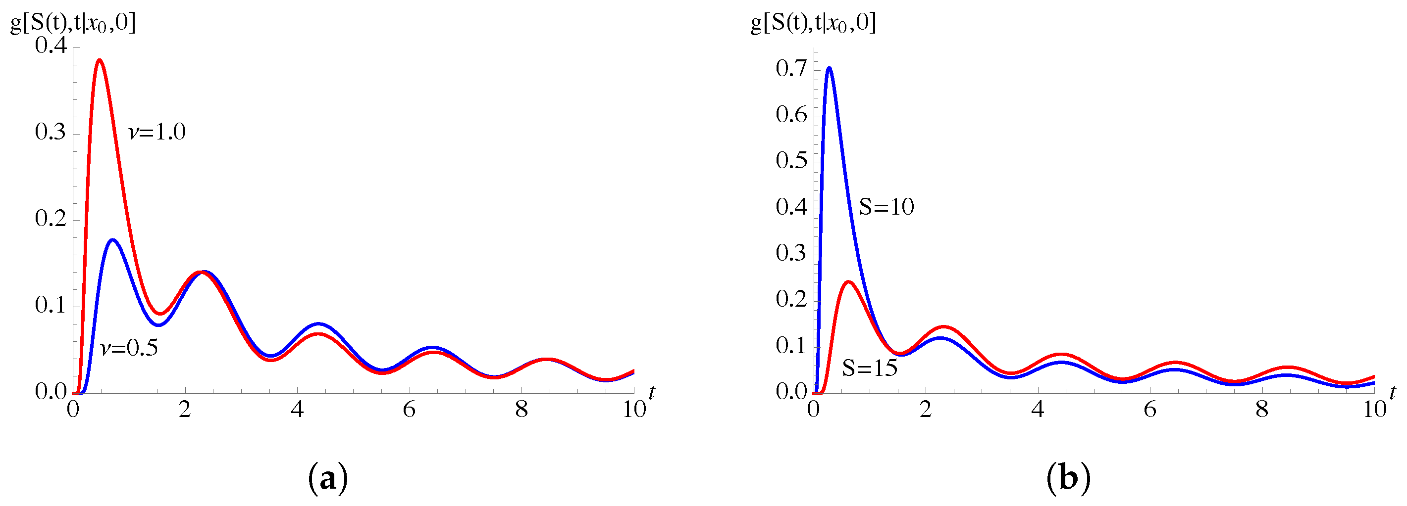
For $\alpha =-0.05$, $c=0.4$ and $Q=2$, in Figure 6, the FPT pdf (83) from $x_0=5$ through $S\left(t\right)=S{e}^{\alpha t}$ is plotted as function of t for different choices of S and ν.

Figure 6. For the Feller-type process having B₁(x,t) = −0.05 x + r(t)/2 and B₂(x,t) = 2r(t)x, with r(t) = ν[1 + 0.4sin(πt)], the FPT pdf (83) from x₀ = 5 through S(t) = Se^αt is plotted as a function of t. (a) FPT pdf for S = 10. (b) FPT pdf for ν = 2.

Proposition 7.

Let $X\left(t\right)$ be a time-inhomogeneous Feller-type diffusion process, having $B_1(x,t)=\alpha \left(t\right)x+3r\left(t\right)/2$ and $B_2(x,t)=2r\left(t\right)x$, with $\alpha \left(t\right)\in \mathbb{R}$, $r\left(t\right)>0$ and a zero-flux condition in the zero state. We assume that $S\left(t\right)=S{e}^{A\left(t\right|0)}$, with $S>0$.

• If $x_0>S\left(t_0\right)>0$, one has:
  $$g[S\left(t\right),t|x_0,t_0]=\frac{r\left(t\right)e^{-A\left(t\right|t_0)}}{\sqrt{\pi {\left[R\left(t\right|t_0)\right]}^3}}\sqrt{\frac{S\left(t_0\right)}{x_0}}\left[\sqrt{x_0}-\sqrt{S\left(t_0\right)}\right]exp\left\{-\frac{{\left[\sqrt{x_0}-\sqrt{S\left(t_0\right)}\right]}^2}{R\left(t\right|t_0)}\right\}$$

  (87)
  and $P\{\mathcal{T}(x_0,t_0)<+\infty \}=\sqrt{S\left(t_0\right)/x_0}$ when ${lim}_{t\to +\infty }R\left(t\right|t_0)=+\infty$.
• If $0<x_0<S\left(t_0\right)$, one obtains:
  $$\begin{array}{ccc}& & g[S\left(t\right),t|x_0,t_0]=\frac{r\left(t\right)e^{-A\left(t\right|t_0)}}{\sqrt{\pi {\left[R\left(t\right|t_0)\right]}^3}}\sqrt{\frac{S\left(t_0\right)}{x_0}}\left[\sqrt{S\left(t_0\right)}-\sqrt{x_0}\right]exp\left\{-\frac{{\left[\sqrt{S\left(t_0\right)}-\sqrt{x_0}\right]}^2}{R\left(t\right|t_0)}\right\}\hfill \\ & & \times \{1+2\sum _{j=1}^{+\infty }exp\left\{-\frac{4j^{2}S\left(t_0\right)}{R\left(t\right|t_0)}\right\}[cosh\left(\frac{4j\sqrt{S\left(t_0\right)}\left(\sqrt{S\left(t_0\right)}-\sqrt{x_0}\right)}{R\left(t\right|t_0)}\right)\hfill \\ & & -\frac{2j\sqrt{S\left(t_0\right)}}{\sqrt{S\left(t_0\right)}-\sqrt{x_0}}sinh\left(\frac{4j\sqrt{S\left(t_0\right)}\left(\sqrt{S\left(t_0\right)}-\sqrt{x_0}\right)}{R\left(t\right|t_0)}\left)\right]\right\}\hfill \end{array}$$

  (88)

  and $P\{\mathcal{T}(x_0,t_0)<+\infty \}=1$ when ${lim}_{t\to +\infty }R\left(t\right|t_0)=+\infty$.
• If $x_0=0$ and $S\left(t_0\right)>0$, one has:

  $$\begin{array}{ccc}& & g[S\left(t\right),t|0,t_0]=\frac{4r\left(t\right)e^{-A\left(t\right|t_0)}\sqrt{S\left(t_0\right)}}{\sqrt{\pi {\left[R\left(t\right|t_0)\right]}^3}}exp\left\{-\frac{S\left(t_0\right)}{R\left(t\right|t_0)}\right\}\sum _{j=1}^{+\infty }jexp\left\{-\frac{4j^{2}S\left(t_0\right)}{R\left(t\right|t_0)}\right\}\hfill \\ & & \times [\frac{4jS\left(t_0\right)}{R\left(t\right|t_0)}cosh(\frac{4jS\left(t_0\right)}{R\left(t\right|t_0)})-\left(1+\frac{2S\left(t_0\right)}{R\left(t\right|t_0)}\right)sinh(\frac{4jS\left(t_0\right)}{R\left(t\right|t_0)}\left)\right]\hfill \end{array}$$

  (89)
  and $P\{\mathcal{T}(x_0,t_0)<+\infty \}=1$ when ${lim}_{t\to +\infty }R\left(t\right|t_0)=+\infty$.

Proof. 

Relations (87)–(89) follow from Proposition 2, making use of (74), (76) and (79). □

Example 2.

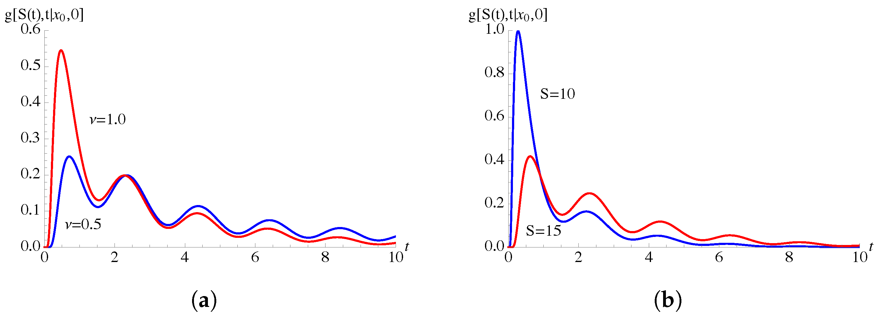
We consider the Feller-type process, having $B_1(x,t)=\alpha x+3r\left(t\right)/2$ and $B_2(x,t)=2r\left(t\right)x$, with $r\left(t\right)$ given in (85). From (70), for $t\ge t_0$ one has $A\left(t\right|t_0)=\alpha (t-t_0)$ and $R\left(t\right|t_0)$ is given in (86). For $\alpha =-0.05$, $c=0.4$ and $Q=2$, in Figure 7, the FPT pdf (88) from $x_0=5$ through $S\left(t\right)=S{e}^{\alpha t}$ is plotted as function of t for some choices of S and ν.

Figure 7. For the Feller-type process, having B₁(x,t) = −0.05 x + 3r(t)/2 and B₂(x,t) = 2r(t)x, with r(t) = ν[1 + 0.4sin(πt)], the FPT pdf (88) from x₀ = 5 through S(t) = Se^αt is plotted as function of t. (a) FPT pdf for S = 10. (b) FPT pdf for ν = 2.

6. Asymptotic Behavior of the FPT Density for a Time-Inhomogeneous Feller-Type Process

In the following proposition, we prove that the FPT density $g[S\left(t\right),t|x_0,t_0]$ of the process (69), with a zero-flux condition in the zero state, is a solution of a second-kind non-singular Volterra integral equation.

Proposition 8.

Let $S\left(t\right)\in C^1[t_0,+\infty )$, with $S\left(t\right)>0$. For the time-inhomogeneous Feller-type diffusion process (69), with $\alpha \left(t\right)\in \mathbb{R}$, $r\left(t\right)>0$ and $\xi >0$, the FPT pdf $g[S\left(t\right),t|x_0,t_0]$ is a solution of the integral Equation (57) with $\varrho =1$ if $x_0<S\left(t_0\right)$ and $\varrho =-1$ if $x_0>S\left(t_0\right)$, where

$$\begin{array}{ccc}& & \Omega [S\left(t\right),t|y,\tau ]=\frac{r\left(t\right)e^{-A\left(t\right|\tau )}}{R\left(t\right|\tau )}exp\left\{-\frac{S\left(t\right)e^{-A\left(t\right|\tau )}+y}{R\left(t\right|\tau )}\right\}{\left[\frac{S\left(t\right)e^{-A\left(t\right|\tau )}}{y}\right]}^{(\xi -1)/2}\hfill \\ & & \times \{\frac{1}{2}\left[-\frac{\alpha \left(t\right)S\left(t\right)}{r\left(t\right)}+\frac{S^{\prime }\left(t\right)}{r\left(t\right)}-\frac{2S\left(t\right)e^{-A\left(t\right|\tau )}}{R\left(t\right|\tau )}+\xi -\frac{1}{2}\right]I_{\xi -1}\left[\frac{2\sqrt{yS\left(t\right)e^{-A\left(t\right|\tau )}}}{R\left(t\right|\tau )}\right]\hfill \\ & & +\frac{\sqrt{yS\left(t\right)e^{-A\left(t\right|\tau )}}}{R\left(t\right|\tau )}{I}_{\xi }\left[\frac{2\sqrt{yS\left(t\right)e^{-A\left(t\right|\tau )}}}{R\left(t\right|\tau )}\right]\}.\hfill \end{array}$$

(90)

Proof. 

The FPT pdf $\widehat{g}[\widehat{S}\left(\widehat{t}\right),\widehat{t}|{\widehat{x}}_0,{\widehat{t}}_0]$ of the process $Y\left(t\right)$, with infinitesimal drift $C_1=\xi$ and infinitesimal variance $C_2\left(\widehat{x}\right)=2\widehat{x}$, with a zero-flux condition in the zero state, is a solution of the following integral equation

$$\begin{array}{ccc}& & \widehat{g}\left\{\widehat{S}\left[h\left(t\right)\right],h\left(t\right)|{\widehat{x}}_0,h\left(t_0\right)\right\}=\rho \{-2\widehat{\Omega }\left\{\widehat{S}\left[h\left(t\right)\right],h\left(t\right)|{\widehat{x}}_0,h\left(t_0\right)\right\}\hfill \\ & & +2{\int }_{h\left(t_0\right)}^{h\left(t\right)}\widehat{g}\left\{\widehat{S}\left(\vartheta \right),\vartheta |{\widehat{x}}_0,h\left(t_0\right)\right\}\widehat{\Omega }\left\{\widehat{S}\left[h\left(t\right)\right],h\left(t\right)|\widehat{S}\left(\vartheta \right),\vartheta \right\}d\vartheta \},{\widehat{x}}_0\ne \widehat{S}\left[h\left(t_0\right)\right],\hfill \end{array}$$

(91)

where, due to (59) with $\beta =\xi$ and $r=1$, one has:

$$\begin{array}{ccc}& & \widehat{\Omega }\left[\widehat{S}\left(v\right),v|z,\vartheta \right]=\frac{1}{v-\vartheta }exp\left\{-\frac{\widehat{S}\left(v\right)+z}{v-\vartheta }\right\}{\left[\frac{\widehat{S}\left(v\right)}{z}\right]}^{(\xi -1)/2}\hfill \\ & & \times \left\{\frac{1}{2}\left[{\widehat{S}}^{\prime }\left(v\right)-\frac{2\widehat{S}\left(v\right)}{v-\vartheta }+\xi -\frac{1}{2}\right]I_{\xi -1}\left[\frac{2\sqrt{z\widehat{S}\left(v\right)}}{v-\vartheta }\right]+\frac{\sqrt{z\widehat{S}\left(v\right)}}{v-\vartheta }{I}_{\xi }\left[\frac{2\sqrt{z\widehat{S}\left(v\right)}}{v-\vartheta }\right]\right\}.\hfill \end{array}$$

(92)

Multiplying both-sides of Equation (91) by $dh\left(t\right)/dt$, performing the transformation $\vartheta =h\left(u\right)$ in the integral and recalling (79), we obtain the integral Equation (57) with

$$\begin{array}{cc}\hfill & \Omega [S\left(t\right),t|x_0,t_0]=\frac{dh\left(t\right)}{dt}\widehat{\Omega }\left\{\widehat{S}\left[h\left(t\right)\right],h\left(t\right)|{\widehat{x}}_0,h\left(t_0\right)\right\},\hfill \\ \hfill & \Omega [S\left(t\right),t|S\left(u\right),u]=\frac{dh\left(t\right)}{dt}\widehat{\Omega }\left\{\widehat{S}\left[h\left(t\right)\right],h\left(t\right)|\widehat{S}\left[h\left(u\right)\right],h\left(u\right)\right\},t_0<u<t.\hfill \end{array}$$

(93)

Then, (90) follows from (93), making use of (74) and (92). □

Let $0\le x_0<S\left(t_0\right)$. We focus on the asymptotic behavior of the FPT pdf of the Feller-type diffusion process (69), with a zero-flux condition in the zero state, through the asymptotically constant boundary (61), with $S\left(t\right)>0$, where $\eta \left(t\right)\in C^1[t_0,+\infty )$ is a bounded function, that does not depend on S, such that (62) holds. We assume that

$$\underset{t\to +\infty }{lim}\alpha \left(t\right)=\alpha <0,\underset{t\to +\infty }{lim}r\left(t\right)=r>0,$$

(94)

so that the process allows a steady-state density. Under such assumptions, from (90), one has:

$$\zeta \left(S\right)=-2\underset{t\to +\infty }{lim}\Omega [S\left(t\right),t|x_0,t_0]=\frac{\left|\alpha \right|S-(\xi -1/2)r}{S\Gamma \left(\xi \right)}{\left(\frac{\left|\alpha \right|S}{r}\right)}^{\xi }exp\left\{-\frac{\left|\alpha \right|S}{r}\right\}.$$

(95)

Finally, by virtue of (57), for $S\to +\infty$ and for long periods, the FPT density through the asymptotically constant boundary (61) of the time-inhomogeneous Feller-type process (69) exhibits the following exponential behavior:

$$g[S\left(t\right),t|x_0,t_0]\simeq \zeta \left(S\right)e^{-\zeta \left(S\right)(t-t_0)},S>\frac{(\xi -1/2)r}{\left|\alpha \right|}·$$

7. Conclusions

In this paper, we have considered the first-passage time problem for a Feller-type diffusion process, having infinitesimal drift $B_1(x,t)=\alpha \left(t\right)x+\beta \left(t\right)$ and infinitesimal variance $B_2(x,t)=2r\left(t\right)x$, defined in $[0,+\infty )$, with $\alpha \left(t\right)\in \mathbb{R}$, $\beta \left(t\right)>0$, $r\left(t\right)>0$ continuous functions. In Section 2, for the time-homogeneous process, we have determined the Laplace transform of the downwards and upwards FPT densities. In Propositions 1 and 2, some connections between the FPT densities for the Feller and the Wiener processes ($\alpha =0$) have been discussed, whereas in Propositions 3 and 4 we have analyzed some relations between the FPT densities for Feller and Ornstein–Uhlenbeck processes ($\alpha \ne 0$). Furthermore, in Section 3, the FPT moments have been investigated by using the Siegert formula. In Section 4, for $\alpha <0$, the asymptotic behavior of the FPT density through a time-dependent boundary has been discussed for an asymptotically constant boundary and for an asymptotically periodic boundary. Furthermore, the first three moments of FPT density through a constant boundary have been compared with the corresponding asymptotic approximations. Section 5 is dedicated to a time inhomogeneous Feller-type diffusion process with $\beta \left(t\right)=\xi r\left(t\right)$, for $\xi >0$. In Propositions 6 and 7, the FPT density has been obtained for an exponential time-varying boundary. The FPT densities have been plotted for periodic noise, showing the presence of damped oscillations having the same periodicity as the noise intensity. In Section 6, a second-kind Volterra integral equation was derived for the FPT density of a time-inhomogeneous Feller-type process through a general time-dependent boundary. Finally, such an equation has been used to derive the asymptotic exponential trend of the FPT pdf through an asymptotically constant boundary.

Analytical, asymptotic and computational methods for the evaluation of FPT densities through time-varying boundaries for more general time-inhomogeneous diffusion processes will be the object of future research focused also on contexts of statistical inference.

References

- Darling, D.A.; Siegert, A.J.F. The first passage problem for a continuous Markov process. Ann. Math. Stat. 1953, 24, 624–639. [Google Scholar] [CrossRef]
- Blake, I.F.; Lindsey, W.C. Level-Crossing Problems for Random Processes. IEEE Trans. Inf. Theory 1973, 19, 295–315. [Google Scholar] [CrossRef]
- Giorno, V.; Nobile, A.G.; Ricciardi, L.M. On the densities of certain bounded diffusion processes. Ric. Mat. 2011, 60, 89–124. [Google Scholar] [CrossRef]
- Di Crescenzo, A.; Giorno, V.; Nobile, A.G.; Ricciardi, L.M. On first-passage–time and transition densities for strongly symmetric diffusion processes. Nagoya Math. J. 1997, 145, 143–161. [Google Scholar] [CrossRef] [Green Version]
- Gutiérrez, R.; Gonzalez, A.J.; Román, P. Construction of first-passage-time densities for a diffusion process which is not necessarily time-homogeneous. J. Appl. Probab. 1991, 28, 903–909. [Google Scholar]
- Di Crescenzo, A.; Giorno, V.; Nobile, A.G. Analysis of reflected diffusions via an exponential time-based transformation. J. Stat. Phys. 2016, 163, 1425–1453. [Google Scholar] [CrossRef]
- Giorno, V.; Nobile, A.G. On the construction of a special class of time-inhomogeneous diffusion processes. J. Stat. Phys. 2019, 177, 299–323. [Google Scholar] [CrossRef]
- Buonocore, A.; Nobile, A.G.; Ricciardi, L.M. A new integral equation for the evaluation of first-passage-time probability densities. Adv. Appl. Probab. 1987, 19, 784–800. [Google Scholar] [CrossRef]
- Gutiérrez, R.; Ricciardi, L.M.; Román, P.; Torrez, F. First-passage-time densities for time-non-homogeneous diffusion processes. J. Appl. Probab. 1997, 34, 623–631. [Google Scholar] [CrossRef] [Green Version]
- Di Nardo, E.; Nobile, A.G.; Pirozzi, E.; Ricciardi, L.M. A computational approach to first-passage-time problems for Gauss-Markov processes. Adv. Appl. Probab. 2001, 33, 453–482. [Google Scholar] [CrossRef]
- Nobile, A.G.; Ricciardi, L.M.; Sacerdote, L. Exponential trends of first passage time densities for a class of diffusion processes with steady-state distribution. J. Appl. Probab. 1985, 22, 611–618. [Google Scholar] [CrossRef]
- Nobile, A.G.; Pirozzi, E.; Ricciardi, L.M. Asymptotics and evaluations of FPT densities through varying boundaries for Gauss-Markov processes. Sci. Math. Jpn. 2008, 67, 241–266. [Google Scholar]
- Herrmann, S.; Zucca, C. Exact simulation of first exit times for one.dimensional diffusion processes. ESAIM Math. Model. Numer. Anal. 2020, 54, 811–844. [Google Scholar] [CrossRef] [Green Version]
- Giraudo, M.T.; Sacerdote, L.; Zucca, C. A Monte Carlo method for the simulation of first passage times of diffusion processes. Methodol. Comput. Appl. Probab. 2001, 3, 215–231. [Google Scholar] [CrossRef]
- Taillefumier, T.; Magnasco, M. A fast algorithm for the first-passage times of Gauss-Markov processes with Hölder continuous boundaries. J. Stat. Phys. 2010, 140, 1130–1156. [Google Scholar] [CrossRef]
- Giorno, V.; Nobile, A.G. On the simulation of a special class of time-inhomogeneous diffusion processes. Mathematics 2021, 9, 818. [Google Scholar] [CrossRef]
- Naouara, N.J.B.; Trabelsi, F. Boundary classification and simulation of one-dimensional diffusion processes. Int. J. Math. Oper. Res. 2017, 11, 107–138. [Google Scholar] [CrossRef]
- Feller, W. Diffusion processes in genetics. In Proceedings of the Second Berkeley Symposium on Mathematical Statistics and Probability, Berkeley, CA, USA, 31 July–12 August 1950; Statistical Laboratory of the University of California: Berkeley, CA, USA, 1950; pp. 227–246. [Google Scholar]
- Lavigne, F.; Roques, L. Extinction times of an inhomogeneous Feller diffusion process: A PDF approach. Expo. Math. 2021, 39, 137–142. [Google Scholar] [CrossRef]
- Masoliver, J. Nonstationary Feller process with time-varying coefficients. Phys. Rev. E 2016, 93, 012122. [Google Scholar] [CrossRef] [Green Version]
- Pugliese, A.; Milner, F. A structured population model with diffusion in structure space. J. Math. Biol. 2018, 77, 2079–2102. [Google Scholar] [CrossRef] [Green Version]
- Di Crescenzo, A.; Nobile, A.G. Diffusion approximation to a queueing system with time-dependent arrival and service rates. Queueing Syst. 1995, 19, 41–62. [Google Scholar] [CrossRef]
- Giorno, V.; Lánský, P.; Nobile, A.G.; Ricciardi, L.M. Diffusion approximation and first-passage-time problem for a model neuron. III. A birth-and-death process approach. Biol. Cyber. 1988, 58, 387–404. [Google Scholar] [CrossRef] [Green Version]
- Buonocore, A.; Giorno, V.; Nobile, A.G.; Ricciardi, L.M. A neuronal modeling paradigm in the presence of refractoriness. BioSystems 2002, 67, 35–43. [Google Scholar] [CrossRef]
- Ditlevsen, S.; Lánský, P. Estimation of the input parameters in the Feller neuronal model. Phys. Rev. E 2006, 73, 061910. [Google Scholar] [CrossRef]
- Lánský, P.; Sacerdote, L.; Tomassetti, F. On the comparison of Feller and Ornstein-Uhlenbeck models for neural activity. Biol. Cybern. 1995, 73, 457–465. [Google Scholar] [CrossRef]
- Nobile, A.G.; Pirozzi, E. On time non-homogeneous Feller-type diffusion process in neuronal modeling. In Computer Aided Systems Theory—Eurocast 2015, LNCS; Moreno-Díaz, R., Pichler, F., Eds.; Springer International Publishing Switzerland: Cham, Switzerland, 2015; Volume 9520, pp. 183–191. [Google Scholar]
- D’Onofrio, G.; Lánský, P.; Pirozzi, E. On two diffusion neuronal models with multiplicative noise: The mean first-passage time properties. Chaos 2018, 28, 043103. [Google Scholar] [CrossRef]
- Cox, J.C.; Ingersoll, J.E., Jr.; Ross, S.A. A theory of the term structure of interest rates. Econometrica 1985, 53, 385–407. [Google Scholar] [CrossRef]
- Tian, Y.; Zhang, H. Skew CIR process, conditional characteristic function, moments and bond pricing. Appl. Math. Comput. 2018, 329, 230–238. [Google Scholar] [CrossRef]
- Maghsoodi, Y. Solution of the extended CIR term structure and bond option valuation. Math. Financ. 1996, 6, 89–109. [Google Scholar] [CrossRef]
- Peng, Q.; Schellhorn, H. On the distribution of extended CIR model. Stat. Probab. Lett. 2018, 142, 23–29. [Google Scholar] [CrossRef]
- Giorno, V.; Nobile, A.G. Time-inhomogeneous Feller-type diffusion process in population dynamics. Mathematics 2021, 9, 1879. [Google Scholar] [CrossRef]
- Ditlevsen, S.; Ditlevsen, O. Parameter estimation from observations of first-passage times of the Ornstein-Uhlenbeck process and the Feller process. Probabilistic Eng. Mech. 2008, 23, 170–179. [Google Scholar] [CrossRef]
- Junginger, A.; Craven, G.T.; Bartsch, T.; Revuelta, F.; Borondo, F.; Benito, R.M.; Hernandez, R. Transition state geometry of driven chemical reactions on time-dependent double-well potentials. Phys. Chem. Chem. Phys. 2016, 18, 30270–30281. [Google Scholar] [CrossRef] [Green Version]
- Fortet, R. Les fonctions aléatoires du type de Markoff associées à certaines équations lineàires aux dérivées partielles du type parabolique. J. Math. Pures Appl. 1943, 22, 177–243. [Google Scholar]
- Giorno, V.; Nobile, A.G.; Ricciardi, L.M.; Sacerdote, L. Some remarks on the Rayleigh process. J. Appl. Probab. 1986, 23, 398–408. [Google Scholar] [CrossRef]
- Linetsky, V. Computing hitting time densities for CIR and OU diffusions. Applications to mean-reverting models. J. Comput. Finance 2004, 7, 1–22. [Google Scholar] [CrossRef] [Green Version]
- Masoliver, J.; Perelló, J. First-passage and escape problems in the Feller process. Phys. Rev. E 2012, 86, 041116. [Google Scholar] [CrossRef] [PubMed] [Green Version]
- Masoliver, J. Extreme values and the level-crossing problem: An application to the Feller process. Phys. Rev. E 2014, 89, 042106. [Google Scholar] [CrossRef] [PubMed] [Green Version]
- Chou, C.-S.; Lin, H.-J. Some Properties of CIR Processes. Stoch. Anal. Appl. 2006, 24, 901–912. [Google Scholar]
- Di Nardo, E.; D’Onofrio, G. A cumulant approach for the first-passage-time problem of the Feller square-root process. Appl. Math. Comput. 2021, 391, 125707. [Google Scholar]
- Giorno, V.; Nobile, A.G. Time-inhomogeneous Feller-type diffusion process with absorbing boundary condition. J. Stat. Phys. 2021, 183, 1–27. [Google Scholar] [CrossRef]
- Feller, W. Two singular diffusion problems. Ann. Math. 1951, 54, 173–182. [Google Scholar] [CrossRef]
- Karlin, S.; Taylor, H.W. A Second Course in Stochastic Processes; Academic Press: New York, NY, USA, 1981. [Google Scholar]
- Sacerdote, L. On the solution of the Fokker-Planck equation for a Feller process. Adv. Appl. Probab. 1990, 22, 101–110. [Google Scholar] [CrossRef]
- Gradshteyn, I.S.; Ryzhik, I.M. Table of Integrals, Series and Products; Academic Press Inc.: Cambridge, MA, USA, 2014. [Google Scholar]
- Tricomi, F.G. Funzioni Ipergeometriche Confluenti. Monografie Matematiche a Cura del Consiglio Nazionale delle Ricerche; Edizioni Cremonese: Roma, Italy, 1954. [Google Scholar]
- Erdèlyi, A.; Magnus, W.; Oberthettinger, F.; Tricomi, F.G. Tables of Integral Transforms; Mc Graw-Hill: New York, NY, USA, 1954; Volume 1. [Google Scholar]
- Abramowitz, I.A.; Stegun, M. Handbook of Mathematical Functions; Dover Publications Inc.: New York, NY, USA, 1972. [Google Scholar]
- Spiegel, M.R.; Lipschutz, S.; Liu, J. Mathematical Handbook of Formulas and Tables; Mc Graw Hill: New York, NY, USA, 2009. [Google Scholar]
- Siegert, A.J.F. On the first passage time probability problem. Phys. Rev. 1951, 81, 617–623. [Google Scholar] [CrossRef]
- Capocelli, R.M.; Ricciardi, L.M. On the transformation of diffusion processes into the Feller process. Math. Biosci. 1976, 29, 219–234. [Google Scholar] [CrossRef]
Publisher’s Note: MDPI stays neutral with regard to jurisdictional claims in published maps and institutional affiliations. |
© 2021 by the authors. Licensee MDPI, Basel, Switzerland. This article is an open access article distributed under the terms and conditions of the Creative Commons Attribution (CC BY) license (https://creativecommons.org/licenses/by/4.0/).