Abstract
This paper explores the application of spatial models to non-life insurance data focused on the multi-risk home insurance branch. In the pricing modelling and rating process, spatial information should be considered by actuaries and insurance managers because frequencies and claim sizes may vary by region and the premium should be different considering this rating variable. In addition, it is relevant to examine the spatial dependence due to the fact that the frequency of claims in neighbouring regions is often expected to be more closely related than those in regions far from each other. In this paper, a comparison between spatial models, such as spatial autoregressive models (SAR), the spatial error model (SEM), and the spatial Durbin model (SDM), and a non-spatial model has been developed. The data used for this analysis are for a home insurance portfolio located in Spain, from which we have selected peril of water coverage.
1. Introduction
Modelling of water damage risk is considered to be one of the most relevant issues when determining home insurance premiums. The role of geographical location and potential spatial structures in determining risk premiums has been of certain interest to researchers. This paper focuses on the application of spatial econometrics to improve the modelling of water peril associated with home insurance policies.
According to Investigación Cooperativa de Entidades Aseguradoras-Spanish Association for Cooperative Research between Insurance Entities and Pension Funds (ICEA), in 2020, approximately 39% of home insurance claims in Spain were due to water damage, 12.9% of which were associated with atmospheric phenomena. Similarly, the German Insurance Association (GDV) showed that, in 2015, 56% of the damage to residential dwellings was water damage. GDV highlighted the serious problems associated with this risk and its underestimation. Damage associated with burst pipes and leaks is the most common cause of water damage throughout Europe [1,2]. A research project from the Canadian Actuarial Institute, dealing specifically with water peril and home insurance rating, emphasises a growing trend of loss claims associated with this risk. This study stresses the need for actuaries to apply new methodologies in home insurance rating for water peril coverage due to factors such as climate change, aging of buildings, inadequate infrastructure, and lifestyle changes.
Noteworthy studies regarding water peril show that the increase in the number of water claims in Sweden is partially explained by geographical area or location. Authors rate territories using generalised linear models (GLM), credibility theory, and smoothing and clustering techniques [3,4]. Another analysis of water damage is the spatial analysis of severity and frequency claims in California. This research shows the differences in the spatial pattern of claims according to zip code, with the aim of helping actuaries and managers to improve the rating process [5].
In the actuarial framework, the application of spatial regression models is considered in the analysis of loss ratio experience in the U.S. crop insurance market [6]. Another interesting actuarial application of spatial econometrics is focused on churn prediction considering spatial factors. This study shows that the probability of cancelling the policy by an insurer is greater if there are insurers who have cancelled a policy nearby [7]. In the Bayesian context, spatial modelling applied to actuarial science has been developed by Gschlößl and Czado [8,9], where the inclusion of spatial effects is considered to model claim frequency and claim size, showing more accurate predictions (car insurance). Within this framework, it is significant to mention the application of the Besag, York, and Mollie (BYM) model to analyse the claim frequency and claim size, taking spatial dependence into account in the pricing process [10].
As may be observed above, water damage risk modelling in insurance is highly relevant, due to the fact that said risk represents substantial losses in the insurance sector, and associations within the sector, institutes of actuaries, and both public and private organisations have expressed their concern about this risk. Study [5] has highlighted the importance of considering spatial analysis associated with said risk, although spatial econometric models were not included in the study—hence, considering these models in water risk pricing and measurement would be of great significance.
Furthermore, as has been reflected in the actuarial field for certain risks such as crop insurance or car insurance, spatial econometric models have been applied, especially in the Bayesian context [8,9,10]. This clearly demonstrates actuaries’ interest in spatial econometrics and the importance of including it as a relevant framework within actuarial science. This paper explicitly introduces spatial econometrics to model water damage risk in the home insurance framework, as no previous study to date related to water damage uses spatial econometrics techniques in its risk analysis. The present work develops the analysis and comparison between spatial models and non-spatial models when the insurance company is modelling water damage. In addition, the spatial dependence and the analysis of the indirect and direct spatial factors are measured. The paper is organised as follows. In Section 2, the pricing process and severity claim modelling are discussed. In Section 3, the spatial autoregressive regression model (SAR), the spatial error model (SEM), and the spatial Durbin model (SDM) are presented. The application to home insurance data using and comparing several models is given in Section 4. Finally, the results are summarised and conclusions are drawn.
2. Pricing Process of Multi-Risk Home Insurance
The complexity of pricing insurance products demands the consideration and adoption of numerous issues or perspectives. One of the fundamental points in the process of non-life insurance pricing is associated with the construction of the rating model based on claim frequency and severity modelling, within which all potential risk factors should be taken into account [11]. Based on this, actuaries construct a multivariate rating system that is adjusted to the risk.
In addition, actuaries calculate the average frequency and severity prediction for each policy; the product of said frequency and severity provides the pure premium or risk premium.
The construction of said models is performed by means of generalised linear models (GLM). This methodology is widely recognised nowadays [12], having become the standard within the non-life insurance industry for the areas of motor vehicles, small businesses, and homes.
The necessary steps usually taken in the construction of said models are the following:
- Analysis, treatment, and knowledge of the probability distribution of data associated with claim amount and frequency.
- Categorisation of the risk factors: the final aim of this is to increase the predictive power of the models.
- Selection of risk factors: a set of variables, which are candidates to be a part of the definitive model, is obtained by means of the simulation of potential models.
- Obtaining the definitive model as a combination of estimated relative weights and different risk factors selected.
- Validation and interpretation of the model: in this phase, the theoretical assumptions that underpin the definitive model are validated. A measurement of the degree of prediction accuracy for the resulting estimated pure premium is thereby obtained.
In the case of home insurance, some of the key factors considered for water coverage when fixing the premium are the age of the building, old buildings, the roof condition, inadequate infrastructure, and the quality of the construction materials. These factors could change depending on the client’s portfolio and other external factors that the actuary may consider interesting to include. Undoubtedly, location characteristics play a vital role in potential damages [3,4].
Actuaries usually include the location as a covariable when modelling claim sizes, but by including the variable in this way, they are unable to measure the expansive effect of the water claim between neighbours. This may be done by applying spatial regression models, which additionally allow the measurement of indirect and direct spatial factors. An example of this, related to water damage, is when a rupture in a pipe in one unit can have repercussions for many neighbouring units. Similarly, dishwashers, a burst pipe, water seepage, or a malfunction in machinery that leads to water damage in one unit frequently damage other units as well. In conclusion, the ripple effect between apartments or buildings when water damage occurs should be analysed when modelling the risk in order to determine the premium.
The ripple effect can be modelled by means of a spatial autoregressive model, in contrast to a linear regression model, in which one key hypothesis is the independence (or at least non-correlation) of observations, and this assumption does not fit when autoregressive models are developed. Spatial econometrics models allow us to analyse the space factors in the errors, direct and indirect effects, spatial dependence, and unobservable factors or omitted variables.
For the reasons mentioned above, in the actuarial context, actuaries should consider spatial regression models such as spatial autoregressive models (SAR), the spatial error model (SEM), or the spatial Durbin Watson (SDM), which could provide a model that is better adjusted to the risks related to water damage.
3. Spatial Autoregressive Models Applied to Severity Modelling and Rating for Home Insurance Data
Spatial regression models are linear regression models that consider the existence of spatial dependence or autocorrelation in the variables being analysed. When spatial dependence is identified in a specific spatial unit, it is relevant to measure the spatial spillover effects associated with the relationship between neighbours. This is an important contribution of these models, as will be shown in their empirical application developed in this paper.
In spatial regression models, spatial dependence emerges when the observed values of a location or region (observation i) depend on the values of observations of neighbouring locations. In this case, the data generating process (DGP) for a conventional, cross-sectional, non-spatial sample of n independent observations that are linearly related to explanatory variables in a matrix X will follow this expression:
The spatial dependence effect could be present in the model in an exogenous or endogenous variable, referred to as substantive dependence. Spatial patterns may also exist within an error or residual term, referred to as nuisance dependence. In these models, a spatial weight matrix, W, which is capable of incorporating the influences between locations or neighbours, is included. One relevant contribution of spatial regression models is that they allow the direct and indirect spatial effects (spillovers) to be quantified. These effects are consequences of the influence between neighbours.
To provide an illustration of how the spatial model can be used to quantify the claim losses associated with water claims in home insurance, one could define water claim losses as a dependent variable and factors such as the age and condition of an apartment and the capital invested in the improvement of an apartment as independent variables. In this case, for a five-storey apartment building in which the penthouse apartment suffers a water claim, the neighbour on the floor below would be directly affected (direct spatial effect). Therefore, the rest of the neighbours on the floors below may also suffer damage (indirect spatial effect). In addition, it could be interesting to analyse the variation in the direct spatial effect and indirect spatial effect if an improvement in the plumbing is carried out in the penthouse.
Following [13], if the actuary wants to consider the spatial dependence between observations at nearby locations or homes, a data generating process might take the form shown below:
Let observations and represent neighbours or homes located in regions nearby.
The first model presented is the spatial autoregressive model (SAR). In this model, the spatial weight matrix, W, is included in the dependent or endogenous variable, as shown below:
In this model, the parameters to be estimated are the usual regression parameters , , and and the additional parameter , being the spatial lag Wy of the endogenous variable. It is relevant to mention that a spatial lag measures the impact of the dependent variable (Y), the explanatory variables (X), or the error term (u) observed in other cross-sectional units j than unit i on the dependent variable of unit i. These can be used to provide extended versions of the SAR model, such as the spatial error model (SEM) or the spatial Durbin model (SDM). In the case of the spatial error model (SEM), the spatial dependence is observed in the error or residual term. The spatial error model allows the consideration of the spatial lags in the disturbance process, being one of the most relevant contributions from spatial models. For example, an important variable (unobservable factors) omitted from a linear regression model, such as the improvement of the infrastructures or buildings of an area, may exert an influence on the dependent variable. The mathematical expression of this model is the following:
Moreover, one extension of previous models is the spatial Durbin model (SDM). This model shows a nested structure of SAR and SEM models. The mathematical expression of this model is as shown:
Finally, in this framework, the estimation of the parameters is a relevant issue, and a number of approaches have been developed; see [14,15,16,17]. LeSage provides more detail about these and other techniques that can aid in the calculation of maximum likelihood estimates. It is relevant to remark that the SDM model nests the SEM and SAR models as a special case.
4. Data Description and Experimental Results
In this paper, home insurance data of water coverage in the Spanish territory in the period 2009–2014 are analysed (Figure 1). The data are from a Spanish insurance company, and for the purposes of this severity analysis study, the amount of claims was considered as a dependent variable, while square metres, the nature of the risk, and unemployment rate were considered as explanatory variables or regressors. The number of policies was 109,105 and of the registers was 401,461. The objective of this study is to provide a case study of the advantages of modelling severity using spatial econometric models.
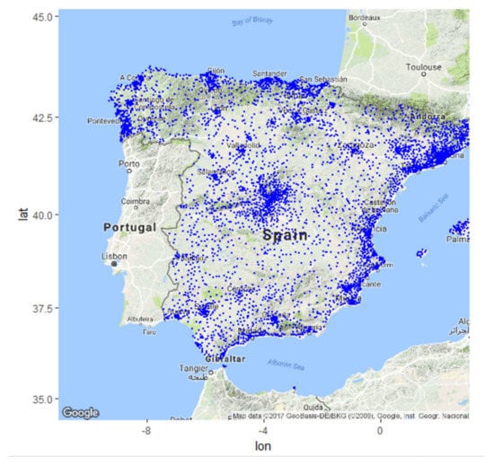
Figure 1.
Geographical distribution of portfolio dwellings throughout Spain.
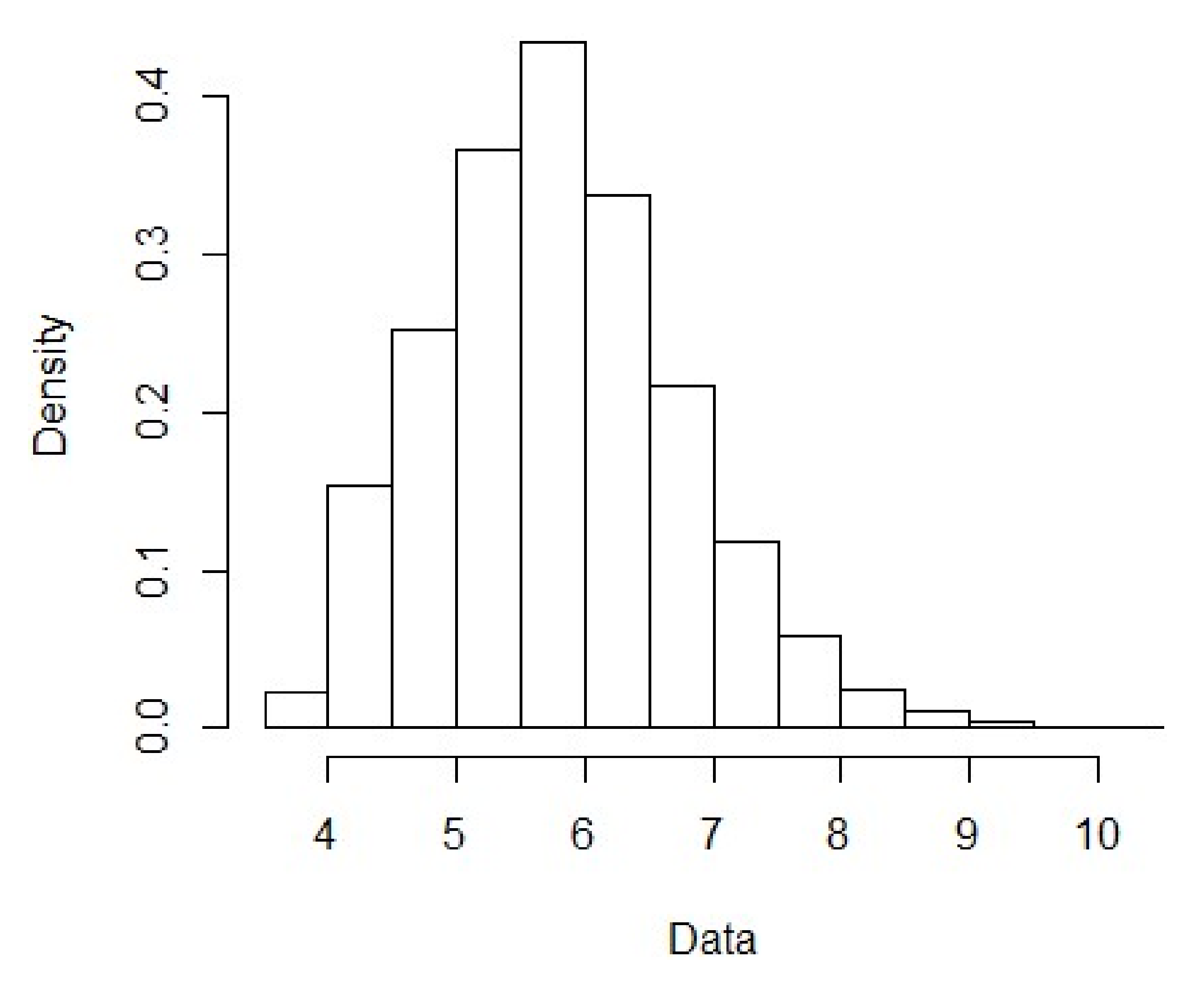
In the study, the logarithm of claim losses was considered in order to analyse the semi-elasticity of losses when a predictor varied (assuming that predictor variables are not in logs, see Figure 2). Moreover, this is more appropriate as the intention is to draw conclusions from the comparison of a linear regression model (baseline) with the spatial econometric models (SAR, SEM, SDM). The predictors selected were square metres, risk nature (detached house, semi-detached, intermediate level apartments, ground floor apartment, penthouse), and unemployment rate. These regressors were selected taking into account the actuarial literature, and it was considered interesting to include a macroeconomic and external variable such as unemployment rate.
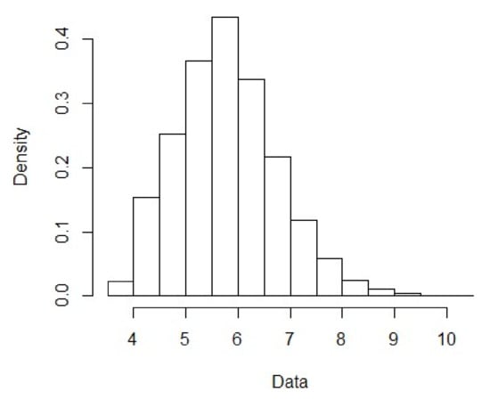
Figure 2.
Histogram of logarithm of incurred losses.
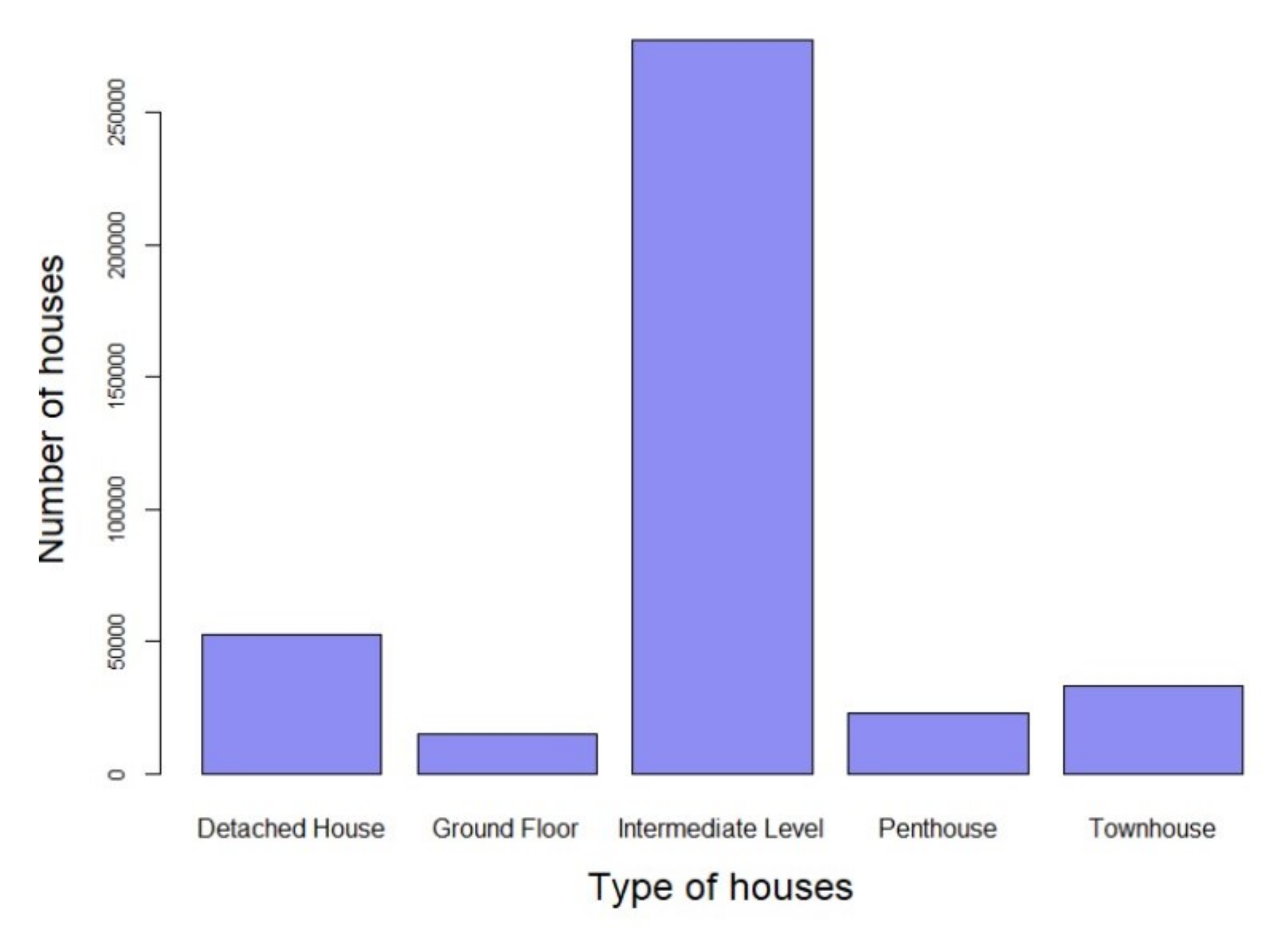
First of all, an exploratory data analysis (EDA) is presented and, afterwards, the models are developed. According to the EDA analysis, most of the homes are between 10 and 15 years old and they are between 90 and 100 m2 (Figure 3). Moreover, most of the homes are intermediate-level apartments (Figure 4).
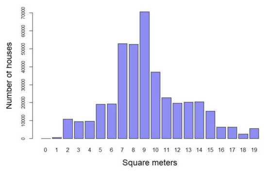
Figure 3.
Distribution of number of dwellings according to square metres.

Figure 4.
Distribution of number of dwellings according to nature of risk.
The dependent variable, incurred, considers the total amount of paid claims and loss reserves associated with a particular period, usually a policy year. In this study, the minimum amount is EUR 50.09 and the maximum is EUR 23,883.66; it is relevant to observe that the volatility of incurred losses is 43%. In the case of the independent variable, square metres, the minimum amount is observed to be 15 square metres, so, in this case, it could be a tiny apartment or storeroom, and the maximum is 325 square metres, which could be a detached house (Table 1). The data on the size of houses are divided into interval groups (sq. m) 00: absent information, 01: 0–30, 02: 30–50, 03: 50–55, 04: 55–60, 05: 60–65, 06: 65–70, 07: 70–80, 08: 80–90, 09: 90–100, 10: 100–110, 11: 110–120, 12: 120–130, 13: 130–150, 14: 150–180, 15: 180–210, 16: 210–240, 17: 240–270, 18: 270–300, 19: 300–higher. It should be noted that the volatility of square metres is 49.5%. In the case of the independent variable, unemployment rate, the minimum rate is 3.13%, and the maximum is 23.43%. This considerable variation makes it relevant to analyse the differences between geographical areas; for this reason, this macroeconomic variable is selected in this study. It should be noted that the volatility of unemployment rate is 40% (Table 1).

Table 1.
Descriptive statistics of dependent and explanatory variables.
The severity is to be modelled by applying a linear regression model and spatial models such as SAR, SEM, and SDM in order to analyse the advantages of implementing spatial models. The SAR includes the spatial lag of dependent variables, the SEM involves the spatial correlation of error terms, and SDM consists of the spatial lag of dependent and independent variables.
The matrix of neighbours was constructed by selecting the closest neighbours according to Euclidean distance. In order to verify the robustness of the results with regard to different matrix specifications, it was decided to select 8, 15, and 25 closest neighbours, repeating the analysis with each matrix of neighbours. In all these cases, the results obtained were similar; therefore, the conclusions may be considered robust, regardless of the number of neighbours selected. The table below details results regarding 25 neighbours obtained once the linear regression model, SAR, SEM, and SDM models were executed. Information with respect to 8 and 15 neighbours can be provided upon request.
The estimation of the parameters was carried out by implementing the maximum likelihood method. This can be seen in pages 45–59 of [13], in which all the details of maximum likelihood estimation, as well as inferences about the estimated parameters, are included. The models were regressed using the package spatialreg in R provided by Bivand [18,19,20]. In order to test the spatial lag, spatial error model, and spatial Durbin model, a comparison of them using the LR test was developed. Moreover, AIC and BIC criteria were considered.
It is interesting to highlight that in this empirical application, our non-spatial regression model shows a spatial pattern in the data and, for this reason, spatial models were considered to be more adequate. Two steps were implemented: first of all, the modelling of this spatial pattern was carried out, after which the selection of the most appropriate spatial model was analysed.
It was observed that all the selected variables were significant in all the models, the variable that most affected the incurred losses being the type of household, specifically semi-detached. Likewise, it could be observed that the unemployment rate affected the claim losses negatively, and this may be associated with the fact that insurance coverage is lower in areas where unemployment rates are higher, and therefore the incurred value may be lower.
Furthermore, these results show that in the linear regression model, Moran’s I is statistically significant, which means that there is spatial autocorrelation in the errors (the residuals). As can be observed, when spatial models are implemented, the spatial autocorrelation of the residuals is not statistically significant, which means that it is possible to state that the errors are not spatially correlated. This is a relevant result because the spatial models remove the spatial dependence of the residuals with respect to a non-spatial model.
The independent variable that most affects the claim amount is the nature of the risk, specifically in the case of a townhouse, both in the direct, indirect, and total effects. Regarding the significance of the impacts, it can be observed that in the case of the SAR model, all impacts are significant. Of note is the negative impact of the unemployment rate on the amount of the claim for water damage, though this could be justified by what was previously mentioned, as in areas with high levels of unemployment, the amount of the claim is lower due to the non-inclusion of certain coverages so as to make the premium cheaper.
With regard to the SDM model and the analysis of its impacts, it can be seen that the variable that most affects the amount of the claim is, as in the previous case, the townhouse, and the unemployment rate also has a negative effect, although the significance of the effects is contradictory and, as has been mentioned previously, is unstable. In addition, impact factors (direct, indirect, and total) of the SAR model are all significant, with the expected sign and magnitude (indirect being smaller than direct, and with the same sign), which also explains the need for spatial modelling of these data. In other words, the conclusions are similar in the three cases, the impacts follow the same pattern, and the results are robust (Table 2 and Table 3).
Table 2.
SAR model results.
Table 3.
SDM model results.
The spatial model clearly selected was SAR against the SEM and SDM models according to Bayesian information criterion (BIC). In this framework, the BIC criterion was selected because this criterion penalised models with a greater number of parameters than AIC and the overestimation was corrected (parsimony principle).
In addition, in the case of the selection between SAR and SDM according to the LR test, SDM was preferred weakly; however, the impacts obtained in the SDM were more unstable than in the SAR model. In the case of the selection between SDM and SEM, SDM was preferred. This can be seen in Table 4 and Table 5.
Table 4.
General results.
Table 5.
Likelihood ratio test.
Due to the above discussion, taking BIC criteria, the stability, and the economic interpretation of the impacts of the SAR model into account, this one has been selected.
Finally, it is relevant to mention that it has been verified, by applying the Jarque Bera test to the residuals, that there are no indications of non-normality. The existence of outliers has also been observed by viewing a q-qplot and a boxplot (available upon request). The sample is quite broad and, therefore, the central limit theorem could be applied, and although the residuals are non-normal, the distribution of estimators may approach a normal one and, thus, the resulting inference is approximately valid, at least from an asymptotic standpoint.
5. Conclusions and Future Research
In this work, spatial econometric models have been defined to model the variable severity of losses associated with insurance policy claims. These spatial models have been applied empirically to non-life home insurance data, specifically home insurance data for water damage coverage.
In the case of the spatial modelling of claim severity, the spatial autoregressive model (SAR), the spatial error model (SEM), and the spatial Durbin model (SDM) have been considered in order to develop a comparison between spatial models and non-spatial model as a baseline. The aim of this perspective is to show the main advantages of taking spatial modelling into account when modelling data claim severity associated with home water coverage claim losses.
After developing the baseline regression model, spatial dependence was observed in the residuals. Given the significance of this fact, SAR, SEM, and SDM models were subsequently applied, and it was noted that the residuals of all the spatial econometric specifications no longer showed any spatial pattern. In addition, all spatial parameters of SAR, SEM, and SDM were also statistically significant. With regard to the selection of the adequate spatial model, the LR test, AIC, and BIC were considered. Eventually, the SAR model was chosen based on the BIC criterion. As is well-known, BIC imposes a strong penalisation for the loss of degrees of freedom and, as a consequence, reduces over-parametrisation against other potential alternatives, such as AIC. With respect to direct and indirect effects, in the SAR model, all of the impacts were statistically significant and the interpretation was clear; however, in the case of SDM, the indirect effects were not statistically significant, likely caused by a potential over-parametrisation of the SDM specification.
It is to be noted that the econometric models applied in this paper allow the spatial patterns present in the data to be gathered. Similarly, they permit the impacts of each variable to be divided into direct and indirect (spatial spillover), as well as to perform the inference of the same. With regard to the selection of SAR as the most adequate model, one argument from a statistical point of view has been that all the spillovers are significant, as was mentioned above, and in both sign and magnitude are as expected according to economic theory. A further statistical argument in favour of the selection of SAR is that it is the model that minimises the BIC.Thus, the need to apply spatial econometric models is strengthened.
It has been shown that the application of the spatial models, in this relevant issue for actuaries, is highly beneficial and greatly improves the modelling process. As has been commented at the start, this work is a study and early application to the pricing process for non-life insurance including spatial factors, although it has been demonstrated that the importance of considering the spatial effect is decisive when fixing a different premium taking into account spatial factors, due to the difference in the nature of the risks.
This analysis could allow a much more accurate premium to be calculated according to the risk assumed, optimising the measurement of said risk by the insurance company. Similarly, an optimum water damage risk measurement could contribute to risk prevention and to loss control for stakeholders (companies, policyholders, governments, society in general). Furthermore, measurement of the direct and indirect impacts of water damage risk could allow the improvement of government policies, thereby enhancing risk prevention and loss control within the risk management process. A further long-term impact of this approach could be a significant improvement in sustainable development, thereby guaranteeing a balance between economic growth, environmental care, and social welfare.
Intended future research includes the improvement of the variable selection using lasso or ridge methods and other spatial semi-parametric alternatives [21,22]. Additionally, future research could be the application to model water risk of the interesting study [23], which proposes a conditional range directional distance estimator by modifying the range directional distance model utilising the probabilistic characterisation of directional distance functions (DDF).
Author Contributions
M.V.R.-L.: Conceptualization, methodology, validation, software, data curation, resources, writing-original draft preparation, writing-review and edition, visualization, project administration, funding acquisition. R.M.-S.: Methodology, validation, supervision, writing-review and edition, visualization. M.M.G.: Conceptualization, Methodology, validation, supervision, writing-review and edition, visualization. A.E.R.: Conceptualization, software. All authors have read and agreed with the published version of the manuscript.
Funding
This research was funded by Universidad Francisco de Vitoria under the project titled “Business analytics, geolocalización y modelización espacial en el sector financiero y asegurador” (Research project funding 2021) and Mariano Matilla-García was funded by the Ministerio de Ciencia e Innovación under grant PID2019-107192GB-I00.
Institutional Review Board Statement
Not applicable.
Informed Consent Statement
Not applicable.
Data Availability Statement
Not applicable.
Conflicts of Interest
The authors declare no conflict of interest.
References
- ICEA. Análisis Técnico de los Seguros Multirriesgo 2019. Available online: https://documentacion.fundacionmapfre.org/documentacion/publico/es/consulta/registro.do?id=121813 (accessed on 30 July 2021).
- Metz, J. Homeowners Insurance for Burst Pipes and Water Leaks. Available online: https://www.forbes.com/advisor/homeowners-insurance/water-damage/ (accessed on 30 July 2021).
- KPMG. Water Damage Risk and Canadian Property Insurance Pricing. Can. Inst. Actuar. 2014. Available online: https://www.cia-ica.ca/docs/default-source/2014/214020e.pdf (accessed on 30 July 2021).
- Emanuelsson, P. Construction of Rating Territories for Water-Damage Claims. Master’s Thesis, Stockholm University, Stockholm, Sweden, 2011. [Google Scholar]
- Singh, G.; Tang, M.; McNeill, D.M.; Hunstad, L. Spatial Distribution of Frequency and Severity of Water Claims in California. J. Actuar. Pract. 2006, 13, 127–146. [Google Scholar]
- Woodard, J.D.; Schnitkey, G.; Sherrick, B.; Lozano-Gracia, N.; Anselin, L. A Spatial Econometric Analysis of Loss Experience in the U.S. Crop. Insur. Program J. Risk Insur. 2012, 79, 261–286. [Google Scholar] [CrossRef]
- Ángel de la Llave, M.; López, F.A.; Angulo, A. The impact of geographical factors on churn prediction: An application to an insurance company in Madrid’s urban area. Scand. Actuar. J. 2019, 2019, 188–203. [Google Scholar] [CrossRef]
- Gschlößl, S.; Czado, C. Spatial modelling of claim frequency and claim size in non-life insurance. Scand. Actuar. J. 2007, 2007, 202–225. [Google Scholar] [CrossRef] [Green Version]
- Brechmann, E.; Czado, C. Spatial Modeling. In Predictive Modeling Applications in Actuarial Science; International Series on Actuarial Science; Frees, E.W., Derrig, R.A., Meyers, G., Eds.; Cambridge University Press: Cambridge, UK, 2014; Volume 1, pp. 260–279. [Google Scholar] [CrossRef]
- Tufvesson, O.; Lindström, J.; Lindström, E. Spatial statistical modelling of insurance risk: A spatial epidemiological approach to car insurance. Scand. Actuar. J. 2019, 2019, 508–522. [Google Scholar] [CrossRef] [Green Version]
- Sharpe, J. Loss Models: From Data to Decisions, 3rd ed.; Klugman, S.A., Panjer, H.H., Willmot, G.E., Eds.; John Wiley & Sons: Hoboken, NJ, USA, 2008; 726p, ISBN 9780470187814. [Google Scholar]
- Goldburd, M.; Khare, A.; Tevet, D.; Guller, D. Generalized Linear Models for Insurance Rating; Casualty Actuarial Society: Arlington, VA, USA, 2020. [Google Scholar]
- LeSage, J.; Pace, R. Introduction to Spatial Econometrics. In Statistics: A Series of Textbooks and Monographs; CRC Press: Boca Raton, FL, USA, 2009. [Google Scholar]
- Besag, J.E.; Moran, P. On the estimation and testing of spatial interaction in Gaussian lattice processes. Biometrika 1975, 62, 555–562. [Google Scholar] [CrossRef]
- Ord, K. Estimation Methods for Models of Spatial Interaction. J. Am. Stat. Assoc. 1975, 70, 120–126. [Google Scholar] [CrossRef]
- Anselin, L. Estimation Methods for Spatial Autoregressive Structures: A Study in Spatial Econometrics; Cornell University Program in Urban and Regional Studies Regional Science Dissertation and Monograph series, Program in Urban and Regional Studies; Cornell University: Ithaca, NY, USA, 1980. [Google Scholar]
- Kelejian, H.H.; Prucha, I. A Generalized Moments Estimator for the Autoregressive Parameter in a Spatial Model. Int. Econ. Rev. 1999, 40, 509–533. [Google Scholar] [CrossRef] [Green Version]
- Bivand, R.; Piras, G. Comparing Implementations of Estimation Methods for Spatial Econometrics. J. Stat. Software Artic. 2015, 63, 1–36. [Google Scholar] [CrossRef] [Green Version]
- Bivand, R.; Hauke, J.; Kossowski, T. Computing the Jacobian in Gaussian Spatial Autoregressive Models: An Illustrated Comparison of Available Methods. Geogr. Anal. 2013, 45, 150–179. [Google Scholar] [CrossRef] [Green Version]
- Bivand, R.; Pebesma, E.; Gómez Rubio, V. Applied Spatial Data Analysis with R; Springer: New York, NY, USA, 2013. [Google Scholar] [CrossRef]
- Basile, R.; Durbán, M.; Mínguez, R.; María Montero, J.; Mur, J. Modeling regional economic dynamics: Spatial dependence, spatial heterogeneity and nonlinearities. J. Econ. Dyn. Control 2014, 48, 229–245. [Google Scholar] [CrossRef]
- Makeienko, M. Symbolic Analysis Applied to the Specification of Spatial Trends and Spatial Dependence. Entropy 2020, 22, 466. [Google Scholar] [CrossRef] [PubMed] [Green Version]
- Tzeremes, P. Productivity, efficiency and firm’s market value: Microeconomic evidence from multinational corporations. Bull. Appl. Econ. 2020, 7, 95–105. [Google Scholar]

Publisher’s Note: MDPI stays neutral with regard to jurisdictional claims in published maps and institutional affiliations. |
© 2021 by the authors. Licensee MDPI, Basel, Switzerland. This article is an open access article distributed under the terms and conditions of the Creative Commons Attribution (CC BY) license (https://creativecommons.org/licenses/by/4.0/).