1. Introduction
The finite mixture probability models have been applied to model heterogeneity in a dataset. For example, Peel and McLachlan [
1] proposed a mixture of
t distributions with the application of clustering multivariate data that contains atypical observations. For more information, the reader may refer to the book by McLachlan and Peel [
2]. Reliability inference is one of the important issues in industrial management to maintain the good quality of productions. In many practical cases, source items are coming from different suppliers, which have been certified, to support the company’s production line. Hence, it is imperative to investigate the mixture type probability model for life testing to deal with the heterogeneity from different resources in industrial reliability analysis. For example, Sultan et al. [
3] explored the mixture of two inverse Weibull distributions and provided some important properties, and Razali and Salih [
4] provided a mixture of two Weibull distributions to analyze the lifetimes of electronic components. Ruhi et al. [
5] investigated the mixture probability model using Weibull distributions as components and provided a case study.
Recent technology advancement has successfully enhanced product reliability. Spending a long time collecting complete lifetime samples from life tests to conduct reliability inference becomes unrealistic under the considerations of the scheduled test time and budget. Different censoring schemes have been adopted in the literature for life testing to conduct reliability inferences; see Balakrishnan and Aggarwala [
6] and Balakrishnan and Cramer [
7] for comprehensive information. Among all censoring schemes developed in industry life testing, the type-I and type-II censoring schemes have earned more attention because of easy implementation. Place
n items on a life test at the same initial time and denote all failure times by
, respectively. Without loss of generality, let the initial time be 0. The life test continues up to the scheduled time
for the type-I censoring scheme; while the life test under the type-II censoring scheme is carried out until a preassigned number,
, of failures is observed. Let
be the ordered lifetimes of the sample
. Then the type-II censoring scheme terminates the life test at lifetime
. Mendenhall and Hader [
8] proposed approximate maximum likelihood estimators (MLEs) of the mixture exponential distributions based on a type II censored sample; while Jones and Ashour [
9] proposed Bayesian estimation method for the mixture exponential distribution parameters to compare with the MLE results. We use the term MLE to denote maximum likelihood estimator/estimate here and after. Amin [
10] proposed a maximum likelihood estimation method for the mixture generalized Rayleigh (GR) distribution under the type-I censoring scheme.
Epstein [
11] presented the type-I hybrid censoring (TIHC) scheme where the life test is ceased at a random time
and Childs et al. [
12] considered the type-II hybrid censoring scheme where the life test is stopped at a random time
. Balakrishnan and Kundu [
13] provided comprehensive discussions regarding the applications of hybrid censoring schemes. More reliability applications about using hybrid censoring schemes can be found in [
14,
15]. Based on our best knowledge, no literature deals with the expectation–maximization MLE (EM-MLE) estimation methods for the mixture distributions model utilizing TIHC samples. In this study, we focus on the applications of using the TIHC scheme for the reliability inferences of the mixture distributions model. Let random variable
D indicate the number of failures by the time
for the TIHC scheme, then,
Moreover, let
denote the censored time of the TIHC scheme; it can be shown that:
Hence, the TIHC sample with the scheduled
r and
can be denoted by
where
indicates
items withdrawn at time
. The EM algorithm is simple to use, and hence the EM algorithm has been widely applied to obtain the MLEs of the model parameters for censoring data and missing data. When the mixture proportions and the data are type-I hybrid censored, it is not easy to obtain the MLE of the model parameters. If the mixture proportions are known, the EM algorithm surely has a better performance than the cases for which the mixture proportions are unknown.
The rest of this article will be structured as follows.
Section 2 addresses the likelihood function using the TIHC sample from the finite mixture distribution. The EM algorithm to find the MLEs of the model parameters and survival function, as well as three bootstrap procedures for confidence intervals, are presented in
Section 2. In
Section 3, a simulation study will be conducted under the mixture model of two-component distributions with Weibull, generalized exponential (GE) and GR distributions. The simulation results will be discussed in
Section 3. Moreover, one numerical TIHC sample is used for illustration.
Section 4 addresses applications by using three examples and
Section 5 provides concluding remarks.
2. Maximum Likelihood Estimation
Let the probability density function (PDF) of lifetimes be
and the cumulative distribution function (CDF) be
, where
is the vector of parameters. Let the realizations of
be denoted by
. The likelihood function based on
can be represented by:
and the log-likelihood function can be presented as:
where
.
In practical applications, the lifetime quality of items could not be consistent. For example, if the items are provided by multiple suppliers and the lifetime quality of items from those suppliers are inconsistent. In the aforementioned situation, a mixture distributions model can be a good candidate for characterizing the lifetimes of items.
2.1. Likelihood Function
Let the lifetimes be taken from a mixture distributions model with
k groups and the PDFs and CDFs of the
k groups be
and
for
. The PDF and CDF of the mixture distributions model can be represented by:
and
respectively, where
is the proportion parameter to indicate the likelihood of the random variable
x from the
jth distribution,
and
. Replacing
and
with Equations (
3) and (
4), Equations (
1) and (
2) can be respectively represented by:
and
The normal equation is obtained as , where is a gradient of with respect to , and is the zero vector with the same dimension of . The MLE of is the solution of . Because of the complicity of the normal equation, the solution procedure is not tractable. The following EM algorithm is suggested to find the MLE of .
2.2. EM Algorithm
For
, let
be the indicator of the lifetime of the
ith tested item being censored or not and defined as:
If
is taken from the
jth distribution, then the contribution to the joint PDF can be presented by:
Define latent variable by
if
is from the
jth distribution; otherwise,
for
and
. Then, the likelihood function of Equation (
5) and log-likelihood function of Equation (
6) can be respectively represented as follows:
and
The following two steps of the EM algorithm can be iteratively used to obtain the MLEs of the model parameters.
The EM algorithm is implemented based on the E-step and M-step until convergence as follows:
At step s,
E-step: Update
by:
for
and
.
M-step: Update
and
, respectively, by
and
2.3. Applications
Three common used lifetime distributions of Weibull, GE and GR are used for illustration. Without loss of generality, it is assumed that the mixture distributions model has two components. For simplification, let here and after.
2.3.1. The Mixture Weibull Distributions
Consider two Weibull distributions as the members for mixture, the PDF and CDF are respectively given by:
and
where
is shape parameter,
is scale parameter and
. Hence,
and
The MLEs of
and
,
are the solutions of the system by letting the Equations (
16) and (
17) be 0.
2.3.2. The Mixture GE Distributions
Consider two GE distributions for mixture, the PDF and CDF are respectively given by
and
where
is shape parameter,
is scale parameter and
. Hence,
and
The MLEs of
and
,
are the solutions of the system by letting the Equations (
18) and (
19) to 0.
2.3.3. The Mixture GR Distributions
Consider two GR distributions for mixture, the PDF and CDF are respectively given by
and
where
is shape parameter,
is scale parameter and
. Hence,
and
The MLEs of
and
,
are the solutions of the system by letting the Equations (
20) and (
21) be 0.
Analogously, the results of mixture Weibull, mixture GE and mixture GR distributions can be extended to the mixture distributions with two different distributions; that is, the mixture Weibull and GE distributions, the mixture Weibull and GR distribution and the mixture GR and GE distributions. We skip the details here to save pages.
2.4. Maximum Likelihood Estimate of Survival Function
From Equation (
4), the survival function at given time
is defined by
Let
denote the MLE of
by using the proposed EM algorithm. Then, the MLE of
can be obtained by the plug-in method and be labeled by:
It is difficult to obtain the confidence intervals of and based on the sampling distribution of and . To overcome this difficulty, the parametric bootstrap percentile (PBP) procedure and two bootstrap correction methods are proposed to obtain approximate confidence intervals of and , respectively.
- (a)
PBP procedure
- Step 1.
Under the TIHC scheme with r and , a TIHC sample,
, is collected from a mixture distribution;
- Step 2.
The MLEs based on TIHC sample from Step 1 is obtained by utilizing the proposed EM algorithm and the MLE is obtained via the plug-in method;
- Step 3.
A bootstrap TIHC sample with r and is drawn from the same mixture distribution with the parameters substituted by . Let the bootstrap TIHC sample be denoted by ;
- Step 4.
The MLEs and are derived based on the bootstrap TIHC sample from Step 3;
- Step 5.
Repeat Step 3 and Step 4 B times, where B is a given large positive number. Label all MLEs by and for ;
- Step 6.
Let , be a B bootstrap MLEs obtained in Step 5 for a parameter considered. The empirical distribution, , of can be obtained. Given , the th empirical quantile, , is defined as the th order statistic, , of , , where is the greatest positive integer less than or equal to . Then an bootstrap percentile confidence interval of can be obtained by .
More information regarding PBP procedure, readers may refer to the books by Efron [
16], Efron and Tibshirani [
17] and Shao and Tu [
18]. The two bootstrap correction methods are presented as follows:
- (b)
Hybrid bootstrap percentile (HBP) procedure Shao and Tu [
18] proposed the HBP procedure is provided as follows:
- Step 1.
Repeat Step 1 to Step 5 of the PBP procedure. Let be the MLE utilizing the original TIHC sample. Moreover, let , be the B bootstrap MLEs of ;
- Step 2.
Let be the empirical distribution of , which is defined by , ;
- Step 3.
Let
be the
th quantile of
, where
. An
HBP confidence interval for
can be obtained as the following interval:
The second bootstrap correction method that can be found in the books by Efron and Tibshirani [
17], as well as in Shao and Tu [
18], is addressed as follows:
- (c)
Bootstrap bias-corrected percentile (BCP) procedure
- Step 1.
Implement the Step 1 of the HBP procedure. Let the empirical distribution, , be constructed based on the bootstrap MLEs , ;
- Step 2.
An
bootstrap BCP confidence interval for parameter
can be obtained by:
where
is standard normal distribution CDF and
.
3. Simulation Study
To evaluate the accuracy of the proposed EM algorithm to obtain the MLEs of model parameters using the censored sample under the TIHC scheme with r and , an intensive simulation study will be conducted in this section. The simulation study will utilize three distributions that include Weibull, GE and GR distributions as the baseline component distributions for the two-component mixture distributions model; that is, . All computation work is obtained via using R codes. R is an open software and can be freely downloaded. Population parameters , mixture proportions = (0.6, 0.4) and (0.75, 0.25), as well as the pre-required failure numbers and , are considered in this simulation study for the sample sizes of and 1000. is taken as the maximum of the 85th percentiles of the two distributions for mixture; that is, .
For each set of simulation inputs, the simulation study was conducted 1000 iterations. The maximal iteration for the convergence of EM algorithm is 50 and
B = 10,000 is used for bootstrap sampling. To evaluate the quality of the MLE
of parameter
, relative bias
and relative squared root of mean square error
are used, where:
and
The simulation results for the MLEs of the model parameters are displaced in
Table 1,
Table 2 and
Table 3.
Table 1,
Table 2 and
Table 3 show that almost all cells of rBias and rsMSE are reduced when either sample size
n or
r increases. For the Weibull mixture distributions model, the high survival function value with small failure time input is underestimated by MLE and two other lower survival function values with large failure time inputs are overestimated by MLEs. For the GE mixture distributions model, the low survival function value with large failure time input is overestimated by MLE and the other two higher survival function values with two smaller failure time inputs are underestimated by MLEs. For the GR mixture distributions model, the survival function at median with the failure time input at median is overestimated by MLE and two other survival function values with either high failure time input or low failure time input are underestimated by MLEs. Generally, except for the small survival function values, the other two higher survival function values can be well estimated by MLEs with small rBias and rsMSE.
To evaluate the interval estimator, the proposed bootstrap procedures of PBP, HBP and BCP described in
Section 2.4 with the
bootstrap sample are used. For each simulation run, the empirical distributions of the MLEs of the distribution parameters and survival functions are constructed based on 10,000 bootstrap samples. Moreover, the confidence intervals of the distribution parameters and survival function are obtained based on the bootstrap methods of PBP, HBP and BCP. The quality of the PBP, HBP and BCP bootstrap methods is evaluated based on the coverage probability (CP) with 1000 confidence intervals. Part of the simulated CPs for
confidence intervals of survival function values based on sample size
and
are given as follows:
For the mixture Weibull distributions model with
,
,
,
,
and
at
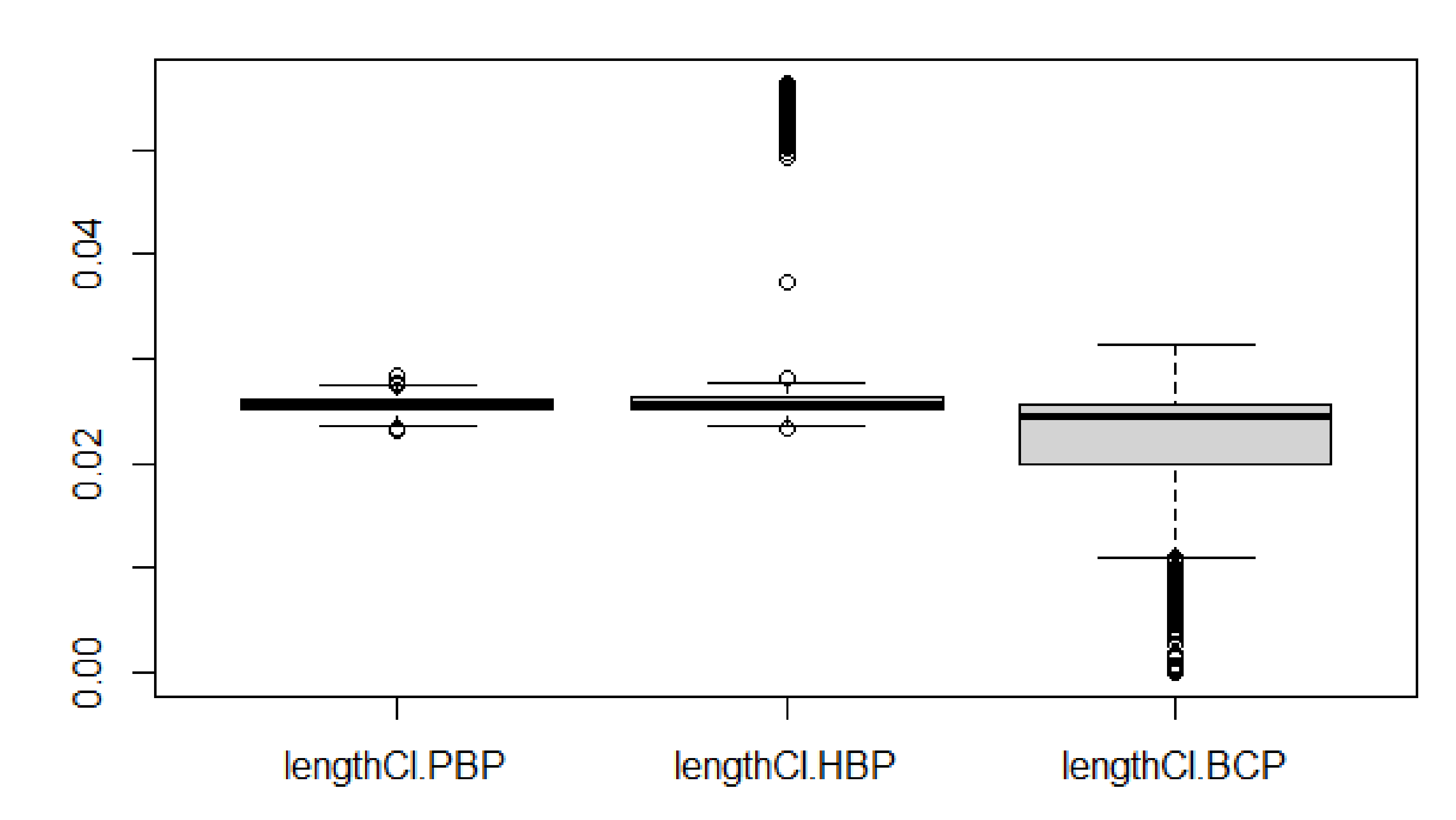
, the
and 0.897 by using PBP, HBP and BCP procedures, respectively.
Figure 1 shows that the lengths of the obtained PBP confidence interval is more consistent than that of the obtained HBP and BCP confidence intervals. The meam length of 1000 confidence intervals based on the PBP, HBP and BCP methods are 0.0256, 0.0286 and 0.0218, respectively.
For the mixture GE distributions model with
,
,
,
,
and
at
, the
and 0.899 by using PBP, HBP and BCP procedures, respectively.
Figure 2 shows that the lengths of the obtained PBP confidence interval are more consistent than those of the obtained HBP and BCP confidence intervals. The meam lengths of 1000 confidence intervals based on the PBP, HBP and BCP methods are 0.0425, 0.0449 and 0.0358, respectively.
For the mixture GR distributions model with
,
,
,
,
and
at
, the
and 0.896 by using PBP, HBP and BCP procedures, respectively.
Figure 3 shows that the lengths of the obtained PBP confidence interval is more consistent than that of the obtained HBP and BCP confidence intervals. The meam lengths of 1000 confidence intervals based on the PBP, HBP and BCP methods are 0.0424, 0.045 and 0.0357, respectively.
Based on the simulation results, the PBP, HBP and BCP methods are competitive, and the PBP method slightly outperforms the other two due to the length of the PBP confidence interval is shorter than that of the other two bootstrap methods.
The simulation study is also conducted to evaluate the PDF and CDF for the three mixture distributions models, which include the mixture model with GR and GE distribution, the mixture model with GR and Weibull distributions, and the mixture model with Weibull and GE distributions. Additional simulation parameter inputs include population parameters and mixture proportion, , (0.50, 0.50). We skip the outputs to save pages. Generally, all the empirical PDFs and CDFs are close to their true function curves.
A simulated example is used to show the applications of the proposed EM-MLE method. The two datasets in
Table 4 present the strength of carbon fibers measured in GPa for single carbon fibers and impregnated 1000-carbon fiber tows; see Murthy et al. [
19] Kundu and Raqab [
20]. These two datasets were originally reported by Badar and Pries [
21] and later studied by Kundu and Raqab [
20]. The first and second datasets contain 63 and 69 strength measurements, respectively, which are tested under tension at gauge lengths of 10 mm and 20 mm. The histograms and empirical density plots are given in
Figure 4.
The Kolmogorov–Smirnov test is used to check the goodness-of-fit of using the Weibull distribution to model these two datasets. The first dataset provides the MLEs and , and the second dataset provides the MLEs and . Replacing the parameters with their MLEs, we obtain the Kolmogorov–Smirnov distances with p-value = 0.965 for the first dataset and with p-value = 0.775 for the second dataset. The testing results indicate that the Weibull distribution can characterize these two datasets well.
These two datasets are not TIHC samples. Assuming a future pool of these two datasets could be coming from a mixture distributions model with Weibull(
,
) and Weibull(
,
) and
. We regenerate a TIHC sample with
and
,
, and
. We are interested in estimating the parameters of the mixture model of two Weibull distributions and the survival function at 0.5(or at
). Utilizing the proposed EM algorithm for the maximum likelihood estimation method and the regenerated sample. The generated TIHC sample is given in
Table 5. The obtained MLEs are
,
,
,
,
and the estimated survival function is
. Using the three proposed bootstrap methods with 5000 iterations to construct the bootstrap empirical distribution of the survival, we obtain the confidence intervals of (0.482, 0.521) for the parametric PBP procedure, (0.474, 0.512) for the HBC procedure and (0.473, 0.513) for the bootstrap BCP procedure.
5. Conclusions and Remarks
In the real world, source items could come from different suppliers to support a company’s production line. The heterogeneity from different resources may cause inconsistencies in the production quality. In these circumstances, it would be more reasonable to utilize a mixture distributions model to characterize the product’s lifetime quality. Moreover, it is very difficult to collect the entire lifetime sample from the life test because of the finite test schedule and restricted budget. Hence, the TIHC scheme with the given failure number r and life test schedule has been proposed for collecting lifetime data from numerous practitioners. In this work, the EM algorithm has been proposed to find the MLEs of the mixture distribution model parameters and the survival function. Three different bootstrap procedures—the PBP, HBC and BCP procedures—are provided to establish the empirical distribution of the MLE of the mixture distribution model parameters and the survival function based on TIHC samples, and to obtain the confidence intervals. The parameter estimation for the mixture distributions model requires a large sample; even the mixture proportions are known with a complete sample. The TIHC scheme renders the sample censored and incomplete. Hence, the proposed EM-MLE requests a very large sample in order to obtain good quality MLEs for the model parameters. This is a drawback of the proposed EM-MLE method, and how to reduce the sample size can be left for future study.
All existing studies on the mixture distributions model have been focused on the mixture of common distributions but with different distribution parameters. In the current work, we extended the EM-MLE method to the mixture distribution model with different distributions as members. The approximate MLE approach proposed by Mendenhall and Hader [
8] is a very interesting procedure for mixture distribution modeling. This will be the focus of a future research project. Meanwhile, the Bayesian estimation approach and some other censoring schemes might provide novel future research potential to add to the mixture distributions model. These two topics will be studied in the future.


