Abstract
This study analyzes the spillover effects of volatility in the Russian stock market. The paper applies the Diebold–Yilmaz connectedness methodology to characterize volatility spillovers between Russian assets. The spectral representation of the forecast variance decomposition proposed by Baruník and Křehlik is used to describe the connectivity in short-term (up to 5 days), medium-term (6–20 days) and long-term (more than 20 days) time frequencies. Additionally, two new augmented models are developed and applied to evaluate conditional spillover effects in different sectors of the Russian economy for the period from January 2012 to June 2021. It is shown that spillover effects increase significantly during political and economic crises and decrease during periods of relative stability. The rising of the overall level of spillovers in the Russian stock market coincides in time with the political crisis of 2014, the intensification of anti-Russian sanctions in 2018 and the fall in oil prices and the start of the pandemic in 2020. With the consideration of the augmented models it can be argued that a significant part of the long-term spillover effects on the Russian stock market may be caused by the influence of external economic and political factors. However, volatility spillovers generated by internal Russian idiosyncratic shocks are short-term. Thus, the proposed approach provides new information on the impact of external factors on volatility spillovers in the Russian stock market.
1. Introduction
The purpose of this paper is to develop new models to analyze volatility spillover across the Russian financial market using an empirical technique for the time and frequency domains.
Over the past 10 years, many studies have investigated volatility spillover, including the interdependence relationships between global and regional markets [1,2], different segments of commodity markets [3,4,5,6,7,8], such as crude oil and the stock markets [9,10,11,12], bonds [13], banks and financial institutions [14], foreign exchange markets and cryptocurrency [15,16,17,18,19,20].
Such studies are aimed at assessing the relationship between the risk of investment in different asset classes, as well as the relationship between firms. The study of volatility is an important aspect of the estimation and modeling of risks, and the connectedness of volatilities can be used in the study of mechanisms and patterns of risk spreading, market, credit and systemic risks management, including fragility, contagion and system risk decomposition.
Recently, a variety of applicable approaches to defining and measuring interconnectedness and interdependence of financial time series have been proposed. For example, the measures based on pairwise correlations or linear Gaussian models have been widely used [21]. Many authors employ pairwise correlations [22,23], GARCH model [24], vector autoregression [25,26], CoVaR [27] and the marginal expected shortfall approach [28]. A large number of works have been devoted to the study of the cumulative effects of the interconnectedness of various market segments based on the analysis of the dynamics of volatility connectedness [2,25,29,30].
In this paper we use the approaches suggested by Diebold and Yilmaz [25] as well as by Baruník and Křehlik [30]. This methods are based on the use of a vector autoregression model for multivariate time series of volatility of a selected subset of assets. The use of the generalized forecast error variance decomposition makes it possible to construct a number of measures of both total and directional volatility spillovers, as well as to carry out decomposition for given time frequencies. Diebold and Yilmaz [29] took the nature of spillovers in a broader context, providing a rigorous framework for measuring spillovers of returns and volatility in financial markets and applying it to determine the effects of volatility propagation. The methodology was applied to measure the effects of connectivity in their follow-up work [31], in which they assessed systemic risk in the US financial sector.
As a characteristic of the connectivity of the system at various levels, from pairwise to system-wide, they proposed to use forecast error variance decomposition for the vector autoregression model. The variance decomposition shows how much of the future uncertainty of asset i is due to shocks in asset j. Variance decomposition is closely related to systemic risk measures such as the marginal expected shortfall [28,32] and CoVaR [27,33] and to various aspects of graph theory.
Representation of a complex system in the form of a graph is a convenient method for its analysis. The constructed graph can be used in various applications including portfolio selection [23], systemic risk analysis [34], stability analysis [35], detection of stock price manipulation [36]. Many studies apply and develop the market graph approach to analyze various structural properties and attributes of financial networks, such as maximum clique, maximum independent sets, degree distribution [37,38,39], clustering [40,41], graph dynamics [42]. The works [35,43] study the financial network’s structural properties and their topological stability, robustness against random vertex failures and fragilities to intentional attacks.
The analysis of network properties is also useful for portfolio investment and risk management, as well as for simplification of the portfolio selection process via targeting a group of stocks or cryptocurrencies belonging to certain regions of the stock market network, and the development of network-based algorithms for analyzing systemic risk [23,31,44,45,46].
Frequency-dependent connectivity measures are usually estimated based on the well-known Generalized Forecast Error Variance Decomposition (GFEVD) [25]. Identifying the interconnectedness in an economic system requires an understanding of its elements connectedness, that appears as responses to economics shocks, for different time-frequency (long, medium and short term). The Diebold and Yilmaz’s approach involves the decomposition of the forecast error over a sufficiently long forecasting period. Baruník and Křehlik [30] proposed a technique for decomposing the forecast variance on selected timeframe. This allows you to highlight the long-term, medium-term, and short-term impacts of a shock, which can conveniently be summed to a total aggregate effect, if needed. For this purpose, the authors defined the spectral representation of generalized forecast error variance decomposition [30].
Many authors touch upon the problem of the influence of macro variables on volatility and volatility jumps [47,48]. For example, the article [49] discusses the dependency of the density of graphs, built on a moving window, on the values of the macro variables.
Diebold’s approach and its extension [25,29,31] were applied to the US financial system, which is the most important part of the global market. In this case it can be assumed that shocks are mainly generated and propagated within the system itself. Presumably, in the case of the Russian stock market, a significant part of the shocks comes from the outside, and they affect companies in different sectors with various strength. If external shocks are not taken into account, then there is a possibility of exaggerating the volatility spillover values within the market. Therefore, we suggest considering augmented VAR models and compare the values of connectivity measures for standard and augmented models. The volatilities of commodity and stock markets were used as exogenous variables.
This approach also allows one to identify the starting moments of turbulence periods in the Russian financial market and to estimate their duration. According to the results of a retrospective analysis, two turbulence periods are well manifested, corresponding to the political crisis of 2014 and the combination of the oil shock and the beginning of the COVID epidemic in early 2020.
The number of studies examining the reaction of financial markets to news related to the development of the COVID-19 pandemic is rapidly increasing [17,50,51,52,53,54].
Our approach allows us to determine what part of the volatility spillovers was caused by the influence of external factors during the crisis. Moreover, we can decompose the total and net spillovers by the selected time frequencies using the proposed approach.
In addition, the cumulative spillover effects of volatility in the commodity and banking sectors on other industries are examined. As one might expect, volatility spillovers from the oil and metallurgical sectors outnumber backward impact from technology or service companies.
In this paper, the proposed tools are applied to describe the relationships between major Russian assets in dynamics before, after and during the financial crises of 2014 and 2020.
The work is organized as follows. Section 2 contains the methodology of spillover measurement. The methods for calculating spillover effects based on generalized forecast error variance decomposition are described. Two new ways to calculate conditional volatility spillovers are introduced. Section 3 describes the data used to measure the connectedness of companies in the RTS Index (RTS—“Russia Trading System”—is a free-float capitalization-weighted index of 50 Russian stocks traded on the Moscow Exchange, calculated in US dollars). In Section 4, a static analysis is carried out which describes the average or unconditional connectivity, while the dynamic conditional connectivity is analyzed using the moving window approach.
2. Methodology
2.1. Spillover Measurement
The methods proposed in this paper are based on the connectedness measurement framework developed by Diebold and Yilmaz [25,29,31]. This approach measures connectedness from three perspectives: total connectedness, total directional connectedness, and pairwise directional connectedness. To construct connectivity measures, the approach uses the decomposition matrices of the forecast variance for a vector autoregression (VAR) model of order p with N variables ():
denotes a intercept vector, are dependent variables, is the matrix of coefficients, is a vector of independently and identically distributed random variables (white noise with (possibly non-diagonal) covariance matrix).
This model assumes that the variables depend on their own lags of the order of p, as well as on the lags of the order p of each of the other variables in the system. Thus, the matrices of coefficients contain comprehensive information about the relationships between variables. It is convenient to work with a polynomial matrix of dimension . Then the model can be rewritten as . Assuming that the roots lie outside the unit circle, the process has the following vector moving average representation :
where the matrices are calculated recursively from the relation :
where is the identity matrix of dimension and for , .
The approach of Koop et al. (1996) and Pesaran and Shin (1998) allows one to find the variance decomposition invariant to the order of variables in the model (GFEVD, generalized forecast error variance decomposition) [55,56]. Note that Pesaran and Shin’s approach for calculating GFEVD can be applyed to different linear and nonlinear multivariate models: VECM, GARCH, TVP-VAR, among many others [16,57,58,59,60,61].
It is possible to denote the expansion of the variance of the forecast error H-step-ahead by for .
Then
where is the variance matrix for the error vector , is the standard deviation of the error for the j-th equation, and is the vector, the i-th of which is equal to one, the rest are zeros.
Following Diebold and Yilmaz, one can measure the connectedness of the system’s variables as follows. Since the sum of the elements in each row of the variance decomposition matrix is not equal to 1: , then to calculate the pairwise spillover indices we should normalize the elements of the decomposition variance matrix:
The overall spillover index is calculated as follows:
The generalized VAR approach allows one to estimate directional measures of volatility spillovers. The directional volatility spillover received by the i asset from all other j assets is calculated using the normalized elements of the generalized variance decomposition matrix:
The directional volatility spillover transmitted by the asset i to all other assets j is calculated in a similar way:
Finally, the net spillovers from the asset i to all other assets of j can be calculated as:
2.2. Time and Frequency Domains of Volatility Spillovers
Baruník and Křehlik used the Fourier transform to generalize the Diebold–Yilmaz approach. They proposed a methodology for decomposition of the spillover effect into different frequency bands [30].
Let us define the function of the frequency response function: , which is derived from the Fourier transform for the coefficients , for .
Frequency connectivity measures based on spectral decomposition of variance are defined as follows:
where is the weight function with respect to the frequency fraction of the variance of the variable j:
which represents the power of the i-th variable at a given frequency.
Decomposition of the variance into components corresponding to given time intervals is determined as follows:
where .
This allows one to find the values of the coefficients for the selected range frequencies d.
2.3. Conditional Spillover Effects
Previous studies have shown the existence of significant cross-country volatility spillovers [62,63,64,65]. In particular paper, ref. [2] has demonstrated that volatility spillovers between the USA and the BRICS countries increase during periods of crises. Moreover, the USA, Brazil, and China are net transmitters, while Russia, India, and South Africa are net receivers of volatility in their respective stock markets. For the net receiver countries, volatility spillovers within their domestic markets are largely due to external influences. Costola and Lorusso identify the booms and busts in the correspondence of political and war episodes that are related to spillover effects in the Russian economy. Their findings show that the Russian Oil and Gas and Metals and Mining sectors are net shock contributors of crude oil and have the highest spillovers to other Russian sectors [66]. Therefore, the Russian stock market should not be viewed as an isolated segment of the global stock market.
It is fair to assume that the movement of prices on world commodity markets and the dynamics of indices of the largest foreign stock markets contain sufficient information about shocks external to the Russian economy. In addition, the impact of foreign markets on the prices of Russian assets far outweighs the reverse impact due to differences in the size of the economy. If these assumptions are correct, then supplementing the econometric model with the appropriate exogenous variables should eliminate the impact of foreign shocks and estimate the conditional spillover effects.
We consider two ways of including foreign shocks for assessing spillover effects.
The first approach of assessing conditional spillover effects is based on a two-step procedure (TS). In the first step, the price volatility of commodities is used as control variables. At the second step, conditional directional spillover effects are calculated using the Equations (3)–(9).
1. First-stage regressions:
where and are the values of the k th initial and exogenous variables for is a vector of coefficients, is an error term.
Let is residuals that we obtain of first stage:
where is OLS coefficient.
2. Second-stage regressions
where .
When using the rolling window approach, the coefficients are estimated once for the full sample. The matrices are evaluated for each of the windows.
The second approach is based on the augmented VAR model (VARX). A vector auto-regressive model with exogenous variables can be expressed as
where are dependent variables, are exogenous variables, and are coefficient matrices, is a vector of independently and identically distributed random variables (white noise with (possibly non-diagonal) covariance matrix).
VARX model representation,
allows us to express the variance of the forecast through the lags of the vector of errors and exogenous variables.
Appendix A contains estimates of conditional volatility spillover for some data generation processes.
If the number of variables is large enough, then the number of estimated parameters grows rapidly depending on the number of lags, and the parameter estimates becomes unstable. In this case, regularization methods can be used for estimation. We use the Least Absolute Shrinkage and Selection Operator (LASSO) for the feature selection and regularization of data models [67].
To reduce the parameter space of the VARX, the VARX-L framework applies structured convex penalties to the least squares VARX problem, resulting in the objective
in which denotes -norm, denotes the norm.
Currently, there is already a sufficient number of works devoted to the problems of using sparse VAR models [68,69,70]. The penalty parameter estimated by sequential cross-validation using algorithms implemented in the BiGVAR package https://cran.r-project.org/web/packages/BigVAR, accessed on 1 July 2021.
3. Data and Preliminary Analysis
We investigate the problem of how volatility spillovers in the Russian stock market depend on different time frequencies. After a preliminary analysis of historical data, 27 large companies included in the RTS Index were selected.
Currently, the RTS index includes the most liquid stocks of the largest Russian issuers. However, some companies included in the RTS Index (for example, CBOM, DSKY, FIVE, LNTA, MOEX, POLY, RNFT, RUAL, SFIN) were not included in our dataset due to a short trading history (about 2–3 years), which is not enough to build an appropriate model. Price data for all companies for the period from 1 January 2012 to 1 June 2021 (2400 trading days) were downloaded from https://finam.ru, accessed on 1 September 2021. 5 min high frequency data were used. In total, the dataset included over 7,000,000 records. Information on the names, tickers of assets and their sector affiliations given in Table 1.

Table 1.
Companies with tickers classified by industry.
Daily volatilities were calculated using 5-min high frequency data.
Let be price of asset i at time t, . Let be its logprice.
Several methods have been proposed for calculating the realized volatility and the realized variance for the whole day for the optimal combination of price volatility in the trading period and overnight. It is well known that the information received during the non-trading period (e.g., overnight) may have a significant impact on volatility [71,72,73,74,75,76]. Hansen and Lunde [71] were the first to propose the method for calculating the whole day variance, as a solution to the problem of optimizing the weights of the square of the profitability of the trading time and night time. Further, Ahoniemi and Lann [74] confirmed the effectiveness of this method using empirical data.
The realized volatility can be calculated in different ways, depending on the data used and the assumptions about price movements during the trading session. Most often, for the computation of volatility, the authors restrict the analysis to daily logarithmic realized volatility, which is computed using 5-min high frequency returns during the trading hours. For the Moscow Exchange in different years, the durations of the trading period were different. Currently, the main trading session runs from 10:00 to 18:50, an additional session from 19:00 to 23:50 Moscow time.
Let be the trading session interval. To calculate the realized volatility for a trading session, the following formula is usually used:
where m is the number of 5-min intervals.
In this case, price movements that occur between the periods of current closing and opening of the next trading session are not taken into account. Let be the overnight return. The value of is usually used as a characteristic of volatility in the period between trading sessions.
Figure 1 shows an example of realized and overnight volatility charts for SBER. Some days overnight price changes significantly exceeded the fluctuations during the trading session. Considering only realized volatility in this case would lead to a significant underestimation of the overall price change per day.
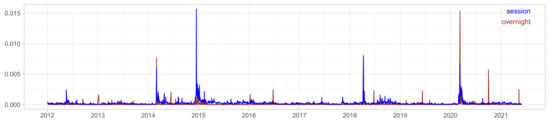
Figure 1.
Realized and overnight volatility for SBER.
For the selected companies, the overnight volatilities are about 1/3 of the intraday volatility, in average. These values roughly correspond to the results of the works [71,74]. Variance for the whole day estimate is based on a combination of realized volatility for the active part of the trades and the square of the overnight yield. Consider a linear combination of and :
where .
The Appendix C shows the values of the weights estimates obtained for the daily volatility. For more than half of the assets, the weights , turned out to be approximately equal to each other. To avoid the overcomplicating the estimation process, we took . As a result, we used an estimate of the realized variance for the whole day without adjustment.
Exogenous variables based on a time series of prices of world commodity markets and US stock indexes (Brent oil futures—ICE BRENT CRUDE OIL PRICES, Gold COMEX, US wheat futures—ZW, LME COPPER, LME NICKEL, SP5000) were constructed. Besides that, 5-min data from https://finam.ru (accessed on 1 July 2021) were used. For time series of commodity markets prices, information is available for the entire 24 h period without interruptions, which allows us to find realized volatility without additional adjustments.
4. Empirical Results
4.1. Spillover Results
Second-order vector autoregression is considered the main model. The method of structured penalized regression (LASSO) is used for its estimation. The forecasting horizon is chosen to be equal to 100 trading days (), the frequency decomposition is carried out for three intervals of H: from 0 to 5 (short-term), from 6 to 20 (medium-term), and from 21 days to 100 trading days (long-term).
A full sample pairwise spillover matrix for VAR model is presented in Table 2. The -th entry corresponds to the -th directional connectivity, that is, the contribution to the variance of the 100-day volatility forecast error for i due to shocks from j.
Table 2.
Full-sample connectedness table.
The column (FROM) displays the average receiving directional connectivity, that is, the average of the off-diagonal elements of each row. The (TO) row provides to the average transferring directional connectivity, that is, the average value of off-diagonal elements of columns. The bottom line (NET = TO − FROM) shows the difference between the transferring and receiving spillover. The bottom-right element (in bold) is the total connectivity (sum over the FROM line or, equivalently, the sum over the TO column).
The lines TO (0; 5], TO (6; 20], TO (20; 100], NET (0; 5], NET (6; 20], NET (21; 100]) represent decomposition of the incoming volatility spillovers by the selected frequencies.
The largest elements of the table are located on the main diagonal (intrinsic connections). The measure of overall connectivity is 83%. Note that there are blocks of high pairwise directional connectivity, as in the case of Oil & Gas companies (ROSN, NVTK, LKOH, GAZP, TATN). In addition to this, the spread of the FROM degree distribution is noticeably smaller than that of the TO degree distribution. Companies of Energy and Financial Services sectors are characterized by positive NET ratios. This suggests that the uncertainty arising in these sectors of the economy is more of an influence on the fluctuations in asset prices of companies from other industries than the opposite effect of other sectors.
Using the TS and VARX approaches allows us to analyze the influence of exogenous variables on each of the original time series. In the case of the TS method, standard procedures based on the values of the adjusted or information criteria can be used to assess the statistical significance of the model and select an informative subset of predictors.
Figure 2 shows the values of the adjusted for the regression models for the full time range. The largest values of the coefficients were obtained for the volatility of shares of large exporters of oil, non-ferrous metals, as well as banks. This is consistent with the hypothesis that the volatility of the stock prices of exporters and financial companies depends on information from foreign markets. For companies focused on the domestic market (Consumer Cyclical, Real Estate, Communications Services), the share of risk that can be explained by external economic factors is noticeably less.
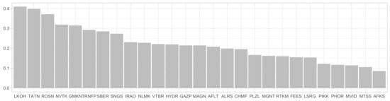
Figure 2.
The value of the for regression models.
The volatility of oil prices was an important factor for the Energy companies, while for the Basic Materials Companies, the metals market volatility turned out to be significant. However, oil price volatility was not an important predictor for financial services companies. The volatility of the US stock markets and the gold market was more important.
The values of the conditional spillover measures, were obtained using the VARX and TS approaches, and us allowed to come to the following conclusions. The total value of NET-effects is not very sensitive to the model’s specification, but the frequency decomposition of volatility depends on whether exogenous variables are included in the model or not. A more detailed analysis of this phenomenon is presented in the next section.
Table 3 presents the decomposition of connectedness.
Table 3.
The decomposition of connectedness.
4.2. Moving-Window Analysis
Analyzing connectivity across the entire sample gives a good estimate of the averaged aspects of each connectivity measure, but does not track changes over time. Therefore, it is also of interest to study interconnectedness in dynamics. One of the most common solutions to this problem is based on the Moving-Window approach. The advantages of this method are the simplicity and consistency with the mechanisms underlying the time-varying parameters. Overlapping windows of 252 calendar days (1 year) width and 1 day increments were taken to track time-varying connectivity in real time.
Diebold–Yilmaz connectivity measures provide aggregated information on how the systemic risk has changed over the period under study. However, it does not show whether shocks affect the system in the short or long term. Therefore, it is of interest to study the frequency sources of connectivity, since it is obvious that the response to shocks from different transmitters is heterogeneous and has different effects on short-term, medium-term and long-term systemic risks.
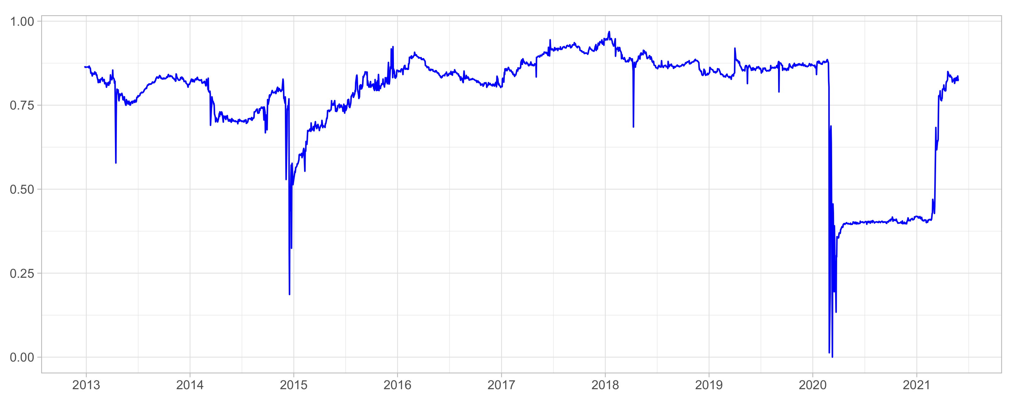
Figure 3 shows the dynamics of the total volatility connectivity index of the system for the VAR model (purple line), and also its decomposition into short-term , medium-term and long-term components. The time on the scale corresponds to the end of the window.
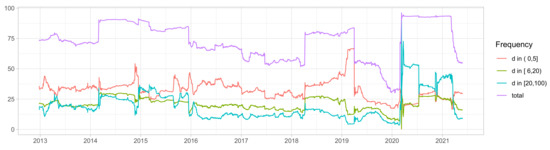
Figure 3.
Dynamic frequency connectedness. DY-BK approach.
The total connectivity in the considered period ranged from 35% to 90%. Large fluctuations in index values can be explained by the different strength and speed of the spread of shocks through the system, for example, weakening of spillover effects during safe periods, or strengthening during periods of political, financial crises, pandemic. During periods of low volatility, the overall connectedness decreased and in crisis periods, on the contrary, it increased.
For example, during the political crisis in Ukraine and the decision to join Crimea to the Russian Federation in 2014, there was an increase in volatility spillovers between Russian assets. The jump in connectivity in the second quarter of 2018 also roughly corresponds in time to the tightening of the sanctions regime against some Russian companies. Peaks in connectivity in 2020 coincide with the beginning of several adverse factors, such as the start of the COVID epidemic and a sharp drop in oil prices. High connectivity persisted for some time after the acute phases of crises. This is typical for both the 2014 political crisis and the 2020 pandemic.
It is important to note that periods of high full connectivity are mainly explained by high-frequency components, with the exception of the period of a pandemic (lockdown, economic closure, a strong drop in oil prices), which is due to the low-frequency component. After periods of crisis, markets begin to stabilize, which reduces uncertainty in low volatility periods and growing markets. This leads to the fact that shocks that create uncertainty in the system in the future will be transmitted much faster, and their impact on the system will be of a short-term nature.
The volatility of volatility has been documented by many authors. To explain this phenomenon, it is suggested that periods, when connectedness is created at high frequencies, are characteristic of financial markets in states of their growth or stability [30]. In this case, markets are able to process information quickly and a shock to one asset affects short-term cyclical behavior. If connectivity appears at lower frequencies, then shocks are transmitted over longer periods. This can be explained by the expectations of investors influencing systemic risk in the long term, which are transferred to other assets in the portfolio. This explanation does not take into account external influences and is correct if the analyzed system is large enough or isolated.
For the past two decades, raw material exporting companies have played a leading role in the Russian economy. The volatility of their shares is significantly influenced by the conjuncture of the world markets for oil, metals, etc. That is, the Russian economy is not closed or isolated, since it is significantly involved in the global exchange of goods through the export of energy resources, raw materials and metals; therefore, volatility shocks in the prices of assets traded in the Russian financial market can be generated by external factors that simultaneously affect more than one asset.
Thus, some volatility spillovers between the Russian assets may be caused by foreign commodity and stock markets fluctuation. The following mechanism of volatility shocks propagation can be assumed. Price shocks in the oil, metals and raw materials markets directly affect the asset prices of Russian exporting companies and indirectly influence the asset prices of all other Russian companies. This leads to a significant overestimation of volatility spillovers for the Energy and Basic Materials sectors. To identify the spillover effects, cleared of the influence of external markets, it is possible either to include in the VAR model exogenous variables reflecting the price volatility of commodity markets, or to try to use indirect methods of estimation. We compared two methods of estimation: VARX and 2-step procedure. Both volatilities and commodity price levels were considered exogenous variables. It is possible that in the short term, price volatility in commodity markets directly affects the price volatility of stocks in exporting companies. Higher or lower prices should lead to a revaluation of the future earnings of exporters.
The following most important explanatory variables were selected: volatility in the prices of oil, gold, aluminum, wheat, volatility of the SP500 index. Price levels turned out to be less important predictors compared to volatility.
The estimation results for TS and VARX methods are presented below. As the final specification of the VARX model, a vector autoregressive model with two lags is chosen.
We use the ratio of total mean squared errors to compare the accuracy of long-term forecasts of different models ( or ):
We denote
We also compare the mean square forecast errors for the volatility of each of the assets for a given horizon. The Table A2 shows the MSE ratio for the DY and VARX models.
The MSE ratios for the DY and VARX models for different time horizons, as well as their rolling estimates for are given in Table A2 and Figure A1 (see Appendix B).
Exogenous factors can explain about 40% of the mean squared errors of long-term forecasts of volatility of oil companies’ stocks, while for companies focused on the domestic market the impact of commodity prices is much weaker. The forecast error using the VARX model is reduced by only 10–20% compared to the VAR model.
For the full sample, we obtain the following estimates: , , that is, exogenous variables explained about 21% of the long-term forecast error.
Figure A1 shows a rolling estimate of the MSE-ratio for the 20-day horizon for the DY and VARX models. The impact of exogenous factors on volatility spillovers in the Russian financial market in 2016–2019 was relatively small. But during the crises of 2014 and 2020, more than half of the fluctuations could be attributed to external factors. Thus, it can be argued that, during stable periods, volatility flows are mainly generated within Russia. During crises, a significant part of volatility flows are due to external factors. As can be noted from the Figure 3, Figure 4 and Figure 5, the values of the total spillover coefficient obtained by the VAR, TS and VARX methods are quite close. However, adding exogenous variables to the model significantly reduces the estimates of conditional medium-term and long-term spillovers during crisis periods. The addition of exogenous variables is most noticeable in the case of VARX.
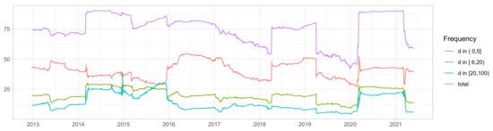
Figure 4.
Dynamic frequency conditional connectedness. Two step approach.
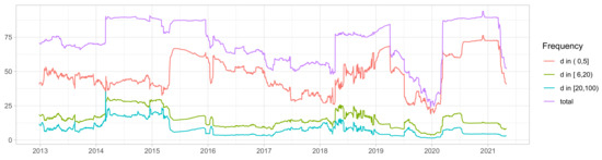
Figure 5.
Dynamic frequency conditional connectedness. VARX approach.
Estimates of conditional medium and long-term spillovers declined both during the economic and political crisis associated with the imposition of sanctions and the fall in oil prices in 2014, and the beginning of the spread of the COVID pandemic in 2020. This testifies in favor of the assumption that the spillover effects of volatility on the Russian stock market can be divided according to the types of shocks that generate them. With the exclusion of external sources of uncertainty, the systemic risk generated directly within the Russian economy spreads rather quickly. More than half of the adaptation takes place within a week, and within a month the influence of almost 85% of overflows is exhausted. In the Figure 4 and Figure 5, the estimate of the long-term component of the total overflow index changes relatively weakly. Generally, the long-term component accounted for less than 15% of the total spillover effect, while in the low volatility periods period of 2016–2018 for less than 5%. Possibly higher estimates of the long-term component of 2014–2015 associated with the fact that the exogenous variables we used not take into account all the features of a given period.
Table 4 shows the average values of the NET coefficients in total and for the frequency (21–100) for all moving windows. The overall NET ratios obtained by all three methods are in good agreement with each other. The positive spillover values for companies in the Energy, Utilities and Financial Services sectors suggest that the risks arising in these sectors spread further to the economy as a whole and outweigh the return flows in terms of their impact. Companies in the Telecommunications and Basic Materials sectors have a negative net ratio. It means that, for these companies, the influence of external sources on risk exceeds in magnitude the outflow of their own risks to the outside.
Table 4.
Overall and long term NET spillovers.
For instance, the coefficient for AFKS is equal to −1.68 and corresponds to the average value of the difference between transmitted and received flows from all other companies (TO = 33.3%, FROM = 78.9%, (33.3 − 78.9)/27 = −1.68). Note that a FROM ratio of around 80% is typical for most companies. But the transmitted spillover is the lowest in our sample. For LKOH, the outgoing effects are much higher than the incoming ones, which are reflected in the positive value of the coefficient (TO = 119.6%, FROM = 85.2%, (119.6 − 85.2)/27 = 1.27). For PIKK, the incoming effects are much higher than the outgoing ones, which is reflected in the negative value of the coefficient (TO = 43.6%, FROM = 72.1%, (43.6 − 72.1)/27 = −1.06). For Sberbank, we get (TO = 118.1%, FROM = 89.2%, (118.1 − 89.2)/27 = 1.07). For all evaluation periods, the net effects for SBER and LKOH remain positive, while AFKS and PIKK are negative. Financial services and Energy sectors have been a source of instability, while Real Estate and Communications companies have had a negative spillover effect.
NET coefficients obtained by the moving window method for AFKS and LKOH, as well as PIKK and SBER are presented in Figure 6 and Figure 7.
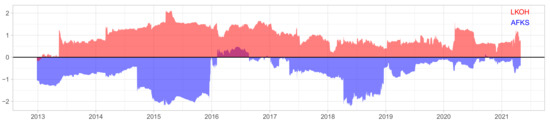
Figure 6.
Net volatility spillover for LKOH and AFKS.

Figure 7.
Net volatility spillover for SBER and PIKK.
Figure 8 and Figure 9 present the results of frequency decomposition for the periods of crises of 2014–2015 and 2020, respectively. In February and March of 2020, the most important external shocks affecting economic processes in the Russian Federation were a sharp drop in oil prices in March 2020, the spread of the COVID pandemic and the imposition of restrictions on population mobility and economic activities. In March 2020, several simultaneous surges in volatility were observed, attributable to the breakdowns of OPEC agreements and a sharp drop in oil prices at the beginning of the month, as well as the official introduction of quarantine measures at the end of the month. The VAR model estimates lead to the conclusion of a sharp and long-term increase in long-term connectivity after the beginning of March 2020. The shocks at the start of the pandemic, as well as the oil crisis, created long-term ties above all. The diminishing of the volatility took several months.
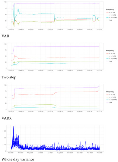
Figure 8.
Dynamic frequency connectedness during period of crisis 2020.
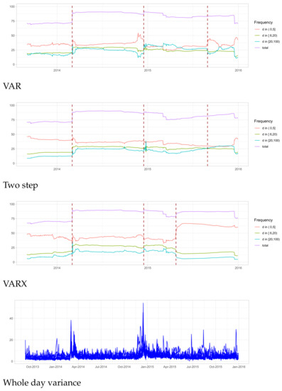
Figure 9.
Dynamic frequency connectedness during 2014–2016.
In contrast, the use of the TS and VARX approaches with the inclusion of exogenous variables (oil, gold, etc.) indicate a fairly quick reaction of the markets. The oil and pandemic shocks were reflected in an increase in the overall interconnectedness by more than 30%, primarily due to the short-term component, and were significantly less pronounced in the medium and long-term relationships. Indeed, for most Russian companies, there was a jump in stock price volatility in March 2020 that was largely abated in a few weeks. The graphs of the realized volatility values for several companies at the beginning of 2020 are given in Figure 8.
Next, we will consider the evolution of the frequency decomposition for the period of the political and economic crisis of 2014 in Russia (Figure 9). The addition of oil and gold price level to exogenous variables did not practically change the interconnection in this time period. One may note that Black Monday (3 March 2014, marked with a dotted line), associated with the political situation in the country, led to an increase in connectivity. At the same time, a more significant jump in medium and long-term connectivity was observed during the period of falling oil prices (from 20 June 2014 to 1 April 2015, marked with dashed lines).
4.3. Directional Volatility Spillovers
The dynamic analysis of the overall connectivity provided an opportunity to elicit the main factors affecting the correlations of the volatility of the pivotal Russian shares in 2012–2021. Thus, it is possible to examine the dynamics of the directional connectivity over time. Figure 10 shows the full directional connectivity (TO and FROM) plots for each company.
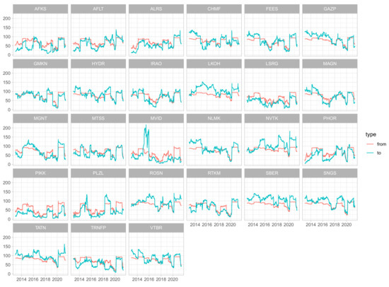
Figure 10.
Overall Directional Connectedness.
The fact that FROM connectivity plots are smoother compared to TO connectivity plots is consistent with previous studies for other [25,77] markets. This is due to how volatility shocks propagate through the system. Idiosyncratic shocks are a significant component of volatility, but some of them have little effect on the volatility of other assets, while others significantly affect the volatility of many stocks in the short or long term. For example, for large companies with strong ties to other companies, the shock can be expected to be passed on to a large number of assets. As a result, individual shocks are more pronounced in the TO coefficient. The FROM indicator reflects the aggregated impact of shocks of all assets, and due to averaging, its fluctuations are weaker.
For most companies, FROM connectivity reached its highest level during the crises of 2014 and 2020. At the same time, a similar level shift in the TO connectivity indicators is not observed. That is, shocks caused by crises first affect individual companies, and then these shocks are transmitted further. During crises, these shocks became more frequent and affected more companies each time than during low volatility periods. None of the companies in our sample is immune to risk spillovers from other organizations and is not exposed to systemic risk.
4.4. Pairwise Directional Spillovers
This section deals with the differences between directed connectivity graphs constructed from the results of evaluating the VAR, TS, VARX model for some periods. The vertices of the graph correspond to the companies, and the edges correspond to the values of the indicators from Equation (9). We simultaneously analyze the indicators of the pairwise-spillover effect as a whole and with a breakdown into short-term, medium-term and long-term components. The first column shows graphs based on short-term relationships; the second column is based on long-term and the third column is based on overall relationships. The graphs corresponding to the frequency from 5 to 20 days are not presented, since they are quite similar to the short-term ones. The lines correspond to different models: VAR, TS, VARX, respectively. Green, orange and gray directional links correspond to the first, fifth and tenth percentile of all net directional links for the periods under consideration. The blue node color corresponds to companies that have a negative NET effect (companies that take shocks), and the red color of the node corresponds to companies with a positive NET effect (companies that distribute shocks). The node size indicates the magnitude of the NET effect in absolute terms.
The structures of graphs built during stable and crisis periods are also compared. Figure 11 shows an example of graphs built from data for the period from 1 March 2015 to1 March 2017. This period of time can be characterized as a period of stable external conditions, a stable level of prices in the markets for raw materials and oil, relatively weak volatility of most of the analyzed time series.
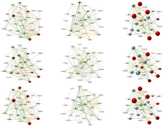
Figure 11.
Frequency decomposition of pairwise volatility spillovers networks (window: from 1 March 2015 to 1 March 2017).
Note that during the low volatility periods, the graphs constructed according to various models are very similar, both for short-term, long-term frequencies, and overall. At the same time, the bulk of communications falls on short-term and medium-term frequencies. The positive NET effect is typical for Energy and Financial Services companies; for companies from other industries, incoming volatility spillovers exceed outgoing ones. Overflows with a frequency of 20 days or more account for less than 10 percent of the total flow. This time period can be considered an example of the behavior of the Russian market in the absence of significant external shocks, when most of the volatility spillovers arise under the influence of events taking place within the Russian economy. Shocks are exhausted in a relatively short period of time (up to 5 or 20 days).
During crises, the frequency of volatility shocks increases. If shocks are caused by external factors, then volatility jumps appear in several or most of the assets at the same time. Figure 12 and Figure 13 show the graphs of directional connections of crisis periods (political crisis of 2014 and oil crisis and COVID in the spring of 2020, respectively).
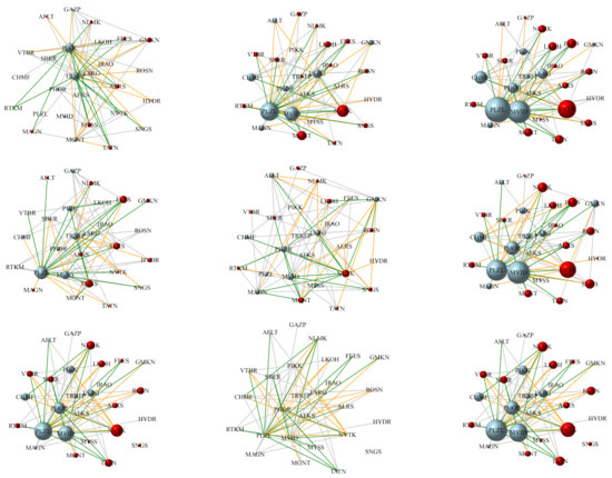
Figure 12.
Net Pairwise Directional Connectedness by pandemic crisis period (from 6 January 2020 to 6 January 2021).
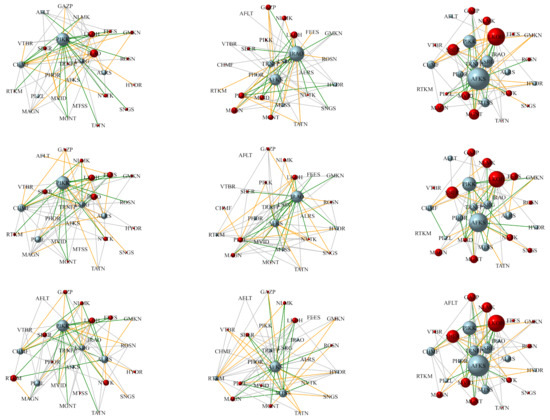
Figure 13.
Net Pairwise Directional Connectedness by politic crisis period (from 1 January 2014 to 1 March 2015).
Note that during crisis periods, the graphs based on overall effects are very close for different model specifications.
The lists of companies that were transmitters and receivers of volatility during two crises of 2014 and 2020 are quite different. Unlike the 2014 crisis, in 2020, in addition to Real Estate and Communications Services, the receivers of volatility were added Consumer Defensive, Consumer Cyclical, Industrials and Basic Materials. In the case of using the VAR model, most of the flows occur on a frequency of a month or more. Those shocks are long term. The addition of exogenous variables (TS and VARX models) to the model leads to a redistribution of a part of the long-term spillover effects in favor of the medium-term and short-term ones.
Volatility spillovers for oil exporting countries have been the subject of analysis by many researchers. For example, Mikhailov [78] analyze the features of the bidirectional volatility spillover effect between the stock and foreign exchange markets for four emerging markets. The results indicate that bidirectional spillover effect turned out to be the most visible in the Russian stock market, because investors in Russian stocks are the most careful and react sharply to bad news and changes in the exchange rate. Pavlova and et.al. [79] study the dynamic spillover of crude oil prices and volatilities on sovereign risk premia of ten oil-exporting countries. The results indicate that Venezuela, Colombia, Russia, and Mexico are the top recipients of crude oil shocks. The effect of political variables, and aggregate demand and supply shocks are relatively less than the oil-specific shocks. The study [80] examines the volatility spillovers between gold, oil futures, and stock markets. Authors find evidence of time-varying volatility spillovers, which are intensified under major events. A portfolio management analysis reveals that a mixed portfolio (commodity and stock markets) provides a higher level of hedging effectiveness for both emerging and developed markets. Kai Shi [81] attempts to comprehensively decode the connectedness among the stock markets of BRICS countries between 1 August 2002 and 31 December 2019 not only in the time domain but also in the frequency domain. The paper shows that China’s and Russia’s stock markets play the influential role for return spillover and volatility spillover across BRICS markets, respectively. Paper [82] examines the direction and extent of the asymmetric volatility connectedness among international equity markets. The authors analyze asymmetric volatility connectedness using realized volatility and identify the magnitude of the volatility spillover and the connectedness in networks. It is shown that macroeconomic shocks increase volatility asymmetry.
As far as we know, no one has previously used the method we have developed in this paper for evaluating conditional spillover effects. In most of the previous studies, time varying spillovers are firstly estimated by the moving window method. Then, the dependence of the spillovers on selected factors [66] is analyzed. This is easy to do for a general spillover. However, if one would like to estimate directional and pairwise effects, then the number of equations becomes too large, which complicates the analysis and the formulation of conclusions. Our approach suggests a uniform way to include in the model the variables that reflect the impact of shocks external to the system under study.
The estimates of conditional spillovers significantly depend on the choice of exogenous variables. The huge number of factors can potentially influence volatility spillovers between Russian assets. Perhaps the use of the FAVAR approach could solve the problem of factors selection. In our study, we choose the exogenous variables based on generally accepted opinions about the most important foreign factors affecting the prices of Russian export goods and cross-border cash flows. However, we did not consider the impact of the government and the Central Bank monetary and fiscal policy. The comparison of the impact of external and internal shocks can be the subject of additional research. To do this, the conditional spillover coefficients should be multiplied by the ratio of the forecast variance of the conditional and unconditional models. This could reveal how the absolute values of spillovers change when exogenous variables are added to the model.
5. Conclusions
This article examines the volatility spillovers between the stocks of the 27 largest Russian assets. The approach proposed in this paper extends:
- the estimation method developed by Francis X. Diebold and Kamil Yilmaz [29] for estimation both total and directional spillovers;
- the Frequency Domains Decomposition technique proposed by Jozef Baruník and Tomas Křehlik [30].
The results of estimating volatility spillovers for the model without exogenous and with exogenous variables were compared. We analyzed 5-minute data on the stock prices of the 27 largest Russian companies from 1 Jaunary 2012 to 1 June 2021. The volatilities of commodity prices and foreign stock markets were used as exogenous variables.
We estimated the parameters of the models, both for the sample as a whole, and using the sliding window method, lasting 1 year with a step of 1 day. Frequency decomposition was performed for the intervals of 0–5 days, 6–20 days, 21 days or more.
In 2012–2021, the transmitters of spillover effects were the companies of Oil and Gas and Financial Services sectors, which, on average, were characterized by positive values of NET-coefficients. Companies from Real Estate, Consumer Cyclical and Communications Services are characterized by negative values of NET-effects. This is consistent with the leading role of the Energy sector as the main provider of export revenues. During periods of stable external economic and political conditions, a large share of the spillovers accounted for the short-term component.
The Russian stock market is closely integrated into the global financial system and, as shown in previous studies, is the net receivers of volatility. Moreover, such spillovers are especially intensified during times of crises in the world commodity and stock markets, as well as periods of increasing political risks. To determine the net effects generated by the domestic risk factors impacts of Russian companies the conditional spillovers were calculated. For this, the basic VAR model was extended by exogenous variables.
In times of crisis, methods that take into account and do not take into account external factors led to significantly different results of frequency decomposition. We present the results of the analysis of the directed relationship graphs for the periods of crises of 2014 and 2020. The crisis of 2014 coincides in time with a period of external political uncertainty, and 2020 with a sharp drop in oil prices and the onset of the COVID pandemic.
Application of the Baruník and Krehlík method without exogenous variables led to the conclusion that the long-term component predominated. However, in the case of adding exogenous variables to the model, conditional overflows were redistributed in favor of short-term ones. This suggests that volatility shocks generated within the Russian economy are absorbed rather quickly (more than 50% per week, 90% per month). However, it takes much longer to overcome external shocks associated with changes in the conjuncture of commodity markets or political crises.
The clusters of companies that are transmitters and receivers of volatility during the crises of 2014 and 2020 do not coincide. In 2020, unlike in 2014, Consumer Defensive, Consumer Cyclical, Industrials and Basic Materials were added to the volatility receivers.
The results of the study provide new information on the impact of external factors on volatility flows in the Russian stock market, the significance of shifts in external and internal transmitters of volatility, switching between low and high volatility modes.
The research results can also be used to assess the potential selection of risk-adjusted portfolios and thus provide new information for investor portfolio decisions.
We believe that comparisons of unconditional and conditional estimates of volatility spillovers can be useful in the assessment and management of systemic risk. Unconditional measures depict the connectivity of asset price volatility without considering the impact of external political or economic factors. Conditional measures allow us, due to the inclusion of exogenous variables in the model, to obtain measures of the connectivity of the system under study, cleared from the influence of the selected factors. In addition, comparing unconditional and conditional networks of financial connectivity allows one to trace the most important links in the sense of systemic risk propagation.
Of course, in future studies, it is advisable to expand the composition of exogenous variables to include a larger number of both external and internal factors. Spillover shocks can result from decisions of the central bank or government, for example, changes in key rate, taxes, tariffs, or measures aimed at supporting specific industries. The inclusion of such variables would allow one to examine the response of the spillovers around financial markets to monetary or fiscal policy shocks.
Author Contributions
Conceptualization, V.B. and A.F.; methodology, V.B.; software, V.B. and A.F.; validation, S.S., V.B. and E.C.; formal analysis, V.B., A.F. and S.S.; writing—original draft preparation, V.B. and A.F.; writing—review and editing, S.S. and E.C.; visualization, A.F. and V.B.; supervision, V.B. All authors have read and agreed to the published version of the manuscript.
Funding
The work was supported by the Russian Science Foundation, Project 19-18-00199.
Institutional Review Board Statement
Not applicable.
Informed Consent Statement
Not applicable.
Data Availability Statement
The data are freely available and was taken from www.finam.ru.
Conflicts of Interest
The authors declare no conflict of interest.
Appendix A. Simulation Study
To show the importance of conditional measures, we examine the processes that generate volatility spillovers by simulation. Suppose the data is generated from the following equations:
where .
We are considering the following cases:
- Bivariate VAR(1) model ();
- Augmented bivariate VAR(1) model ();
- Augmented bivariate VAR(1) model with autocorrelated exogenous variable ();
- Three-variable vector autoregressive model:where ().
The length of the simulated time series is . The estimates are computed averaging over the 100 simulations, and the standard error is the sample standard deviation. The simulations are carried out with the given values of the following parameters: , , .
We start with the bivariate autoregressive case with uncorrelated errors. Further, we assume that the exogenous variable is . Then the data generation process can be represented as with error covariance matrix:
For this model, all assumptions of the Diebold–Yilmaz approach are fulfilled, and the Baruník-Křehlik method can be used for spectral representation for variance decompositions.
We then consider the case where the exogenous variable is generated by AR(1) processe with . Finally, we assume that the variable z is endogenous (, , ).
The purpose of the simulation example is to demonstrate the consequences of restrictions when choosing the composition of time series for assessing volatility spillovers. Variables correspond to the subset of indicators selected for analysis. The variable z reflects the influence of factors external to the system under consideration. We analyze 4 cases: there are no external factors (model (i)); exogenous non-autocorrelated external variables (model (ii)); exogenous variables with time dependency (model (iii)); endogenous external factors (model (iv)).
For cases (iii) and (iv), assumption DY does not hold, so we use the methods described in Section 2.3 for estimating conditional spillovers. As exogenous variables, we used . Thus, the regression equations used in the first step of the TS procedure were as follows:
Also, in the augmented vector autoregression model, the variable z and its first lag were used. The results obtained by simulations are presented in Table A1.
Table A1.
Simulation results.
Table A1.
Simulation results.
| Model | Total | (0, 5) | (6, 20) | (21, 100) |
|---|---|---|---|---|
| (i) | ||||
| DY-BK | 20.322 | 2.435 | 8.475 | 9.413 |
| (1.239) | (0.142) | (0.38) | (0.896) | |
| (ii) | ||||
| DY-BK | 20.295 | 2.413 | 8.45 | 9.431 |
| (1.353) | (0.173) | (0.475) | (0.917) | |
| TS | 20.319 | 2.415 | 8.462 | 9.441 |
| (1.139) | (0.161) | (0.401) | (0.776) | |
| VARX | 20.319 | 2.415 | 8.462 | 9.441 |
| (1.14) | (0.161) | (0.402) | (0.776) | |
| (iii) | ||||
| DY-BK | 27.144 | 2.14 | 9.324 | 15.68 |
| (1.318) | (0.152) | (0.406) | (1.164) | |
| TS | 20.468 | 2.415 | 8.496 | 9.557 |
| (1.255) | (0.171) | (0.423) | (0.816) | |
| VARX | 20.468 | 2.415 | 8.496 | 9.557 |
| (1.256) | (0.171) | (0.424) | (0.816) | |
| (iv) | ||||
| DY-BK | 45.049 | 0.479 | 2.071 | 42.5 |
| (0.758) | (0.062) | (0.481) | (1.277) | |
| TS | 20.419 | 2.418 | 8.495 | 9.506 |
| (0.955) | (0.147) | (0.352) | (0.604) | |
| VARX | 20.418 | 2.418 | 8.494 | 9.505 |
| (0.954) | (0.147) | (0.352) | (0.604) | |
Under the assumption of the Diebold and Yilmaz model unconditional and conditional volatility spillovers are close to theoretical values.
However, if external factors are generated by the autoregression process (), then the spillovers found by the DY-BK method change significantly. The value of the long-term component changes especially noticeably. For the four considered models of data generation processes, the average values of the long-term component were respectively 9.413; 9.431; 15.68; 42.50.
The methods we have proposed in Section 2.3 for assessing conditional spillover effects (TS, VARX) make it possible to obtain estimates that are close to theoretical ones.
Note that the estimates obtained by the TS and VARX methods practically coincide.
However, when analyzing real data, we performed the first step of the TS procedure for the entire sample. The second step is either for the sample as a whole, or for sliding windows with a step-by-step procedure for selecting predictors. This made it possible to guarantee the participation of exogenous variables in the estimation process. In the case of the rolling window and VARX procedure, the same weights were used for both endogenous and exogenous variables of the LASSO method. Therefore, for some windows, not all exogenous variables in each of the equations of the VARX model could be used.
Appendix B. The Mean Squared Error Ratio of the h-Step Forecast
Table A2.
Mean square error ratio of the h-step forecast for full sample.
Table A2.
Mean square error ratio of the h-step forecast for full sample.
| Ticker | (0;5] | (0;20] | (0;100] |
|---|---|---|---|
| AFKS | 0.97 | 0.92 | 0.91 |
| MTSS | 0.95 | 0.9 | 0.89 |
| MVID | 0.92 | 0.88 | 0.88 |
| PHOR | 0.93 | 0.88 | 0.87 |
| PIKK | 0.92 | 0.88 | 0.87 |
| FEES | 0.91 | 0.84 | 0.83 |
| MGNT | 0.88 | 0.83 | 0.82 |
| LSRG | 0.89 | 0.82 | 0.82 |
| PLZL | 0.89 | 0.81 | 0.81 |
| RTKM | 0.88 | 0.81 | 0.81 |
| ALRS | 0.88 | 0.8 | 0.79 |
| AFLT | 0.85 | 0.78 | 0.78 |
| HYDR | 0.87 | 0.78 | 0.77 |
| CHMF | 0.85 | 0.78 | 0.77 |
| MAGN | 0.86 | 0.77 | 0.77 |
| GAZP | 0.81 | 0.77 | 0.76 |
| VTBR | 0.84 | 0.76 | 0.76 |
| NLMK | 0.83 | 0.76 | 0.75 |
| IRAO | 0.87 | 0.73 | 0.71 |
| SNGS | 0.8 | 0.71 | 0.71 |
| SBER | 0.78 | 0.71 | 0.7 |
| TRNFP | 0.8 | 0.7 | 0.69 |
| GMKN | 0.78 | 0.68 | 0.67 |
| NVTK | 0.75 | 0.67 | 0.66 |
| ROSN | 0.7 | 0.61 | 0.61 |
| TATN | 0.68 | 0.59 | 0.59 |
| LKOH | 0.67 | 0.58 | 0.58 |
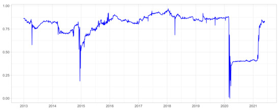
Figure A1.
Dynamic .
Figure A1.
Dynamic .
Appendix C. Optimal Measure of Daily Volatility
We shall employ the estimator that Hansen & Lunde (2005) [71] refer to as the Newey-West modified realized variance:
The optimal weights were calculated as follows
- ,
- ,
- where
- , , , , , ,
- .
To find the parameter , robust estimates were used.
Table A3.
Optimal measure of daily volatility: Empirical estimates of components.
Table A3.
Optimal measure of daily volatility: Empirical estimates of components.
| TICKER | ||||||||||
|---|---|---|---|---|---|---|---|---|---|---|
| 1 | AFKS | 10.442 | 2.142 | 10.371 | 16.588 | 39.898 | 0.214 | 0.802 | 0.965 | 0.808 |
| 2 | AFLT | 5.516 | 0.989 | 5.458 | 4.581 | 11.601 | 0.152 | 0.827 | 0.966 | 0.836 |
| 3 | ALRS | 5.393 | 0.716 | 5.278 | 2.709 | 9.006 | 0.129 | 0.832 | 1.264 | 0.850 |
| 4 | CHMF | 3.860 | 0.716 | 3.823 | 4.032 | 5.773 | 0.075 | 0.934 | 0.358 | 0.943 |
| 5 | FEES | 6.441 | 1.035 | 6.359 | 4.342 | 13.505 | 0.158 | 0.797 | 1.265 | 0.807 |
| 6 | GAZP | 2.745 | 0.613 | 2.725 | 4.232 | 6.318 | 0.038 | 0.899 | 0.452 | 0.906 |
| 7 | GMKN | 3.447 | 0.677 | 3.403 | 2.533 | 6.770 | 0.063 | 0.780 | 1.118 | 0.791 |
| 8 | HYDR | 4.464 | 0.677 | 4.442 | 3.222 | 8.844 | 0.078 | 0.852 | 0.977 | 0.856 |
| 9 | IRAO | 6.353 | 0.920 | 6.234 | 4.922 | 14.955 | 0.143 | 0.833 | 1.153 | 0.849 |
| 10 | LKOH | 3.067 | 0.637 | 3.025 | 6.335 | 8.537 | 0.038 | 0.926 | 0.358 | 0.939 |
| 11 | LSRG | 8.289 | 1.083 | 8.128 | 5.391 | 13.590 | 0.224 | 0.899 | 0.770 | 0.917 |
| 12 | MAGN | 5.102 | 0.811 | 5.045 | 3.437 | 7.711 | 0.119 | 0.886 | 0.717 | 0.896 |
| 13 | MGNT | 4.599 | 0.756 | 4.550 | 4.790 | 8.285 | 0.076 | 0.924 | 0.462 | 0.934 |
| 14 | MTSS | 3.767 | 0.747 | 3.725 | 3.840 | 8.378 | 0.052 | 0.840 | 0.808 | 0.849 |
| 15 | MVID | 8.145 | 1.402 | 8.098 | 10.795 | 19.595 | 0.257 | 0.910 | 0.521 | 0.916 |
| 16 | NLMK | 4.423 | 0.732 | 4.363 | 2.643 | 6.376 | 0.096 | 0.861 | 0.842 | 0.873 |
| 17 | NVTK | 4.626 | 0.764 | 4.584 | 5.419 | 11.114 | 0.067 | 0.896 | 0.632 | 0.904 |
| 18 | PHOR | 8.341 | 0.824 | 8.124 | 3.055 | 20.793 | 0.159 | 0.678 | 3.262 | 0.696 |
| 19 | PIKK | 6.408 | 0.653 | 6.355 | 2.851 | 14.462 | 0.095 | 0.787 | 2.092 | 0.793 |
| 20 | PLZL | 8.268 | 1.054 | 8.174 | 4.523 | 19.326 | 0.124 | 0.768 | 1.824 | 0.776 |
| 21 | ROSN | 3.238 | 0.742 | 3.212 | 6.202 | 8.434 | 0.061 | 0.911 | 0.391 | 0.918 |
| 22 | RTKM | 3.599 | 0.611 | 3.570 | 3.744 | 8.950 | 0.052 | 0.857 | 0.843 | 0.864 |
| 23 | SBER | 3.501 | 0.838 | 3.476 | 4.286 | 8.022 | 0.086 | 0.832 | 0.704 | 0.838 |
| 24 | SNGS | 4.124 | 0.680 | 4.079 | 6.151 | 10.414 | 0.053 | 0.926 | 0.447 | 0.937 |
| 25 | TATN | 4.654 | 0.788 | 4.586 | 4.915 | 8.314 | 0.089 | 0.923 | 0.457 | 0.936 |
| 26 | TRNFP | 4.778 | 0.564 | 4.720 | 3.277 | 9.757 | 0.084 | 0.888 | 0.946 | 0.899 |
| 27 | VTBR | 3.601 | 0.639 | 3.562 | 3.471 | 6.263 | 0.063 | 0.906 | 0.530 | 0.916 |
References
- Ng, A. Volatility spillover effects from Japan and the US to the Pacific–Basin. J. Int. Money Financ. 2000, 19, 207–233. [Google Scholar] [CrossRef]
- McIver, R.P.; Kang, S.H. Financial crises and the dynamics of the spillovers between the U.S. and BRICS stock markets. Res. Int. Bus. Financ. 2020, 54, 101276. [Google Scholar] [CrossRef]
- Wu, F.; Guan, Z.; Myers, R.J. Volatility spillover effects and cross hedging in corn and crude oil futures. J. Futur. Mark. 2011, 31, 1052–1075. [Google Scholar] [CrossRef]
- Roy, R.P.; Sinha Roy, S. Financial contagion and volatility spillover: An exploration into Indian commodity derivative market. Econ. Model. 2017, 67, 368–380. [Google Scholar] [CrossRef]
- Yip, P.S.; Brooks, R.; Do, H.X.; Nguyen, D.K. Dynamic volatility spillover effects between oil and agricultural products. Int. Rev. Financ. Anal. 2020, 69, 101465. [Google Scholar] [CrossRef]
- Yoon, S.M.; Al Mamun, M.; Uddin, G.S.; Kang, S.H. Network connectedness and net spillover between financial and commodity markets. N. Am. J. Econ. Financ. 2019, 48, 801–818. [Google Scholar] [CrossRef]
- Al-Yahyaee, K.H.; Mensi, W.; Sensoy, A.; Kang, S.H. Energy, precious metals, and GCC stock markets: Is there any risk spillover? Pac.-Basin Financ. J. 2019, 56, 45–70. [Google Scholar] [CrossRef]
- Jiang, Y.; Fu, Y.; Ruan, W. Risk spillovers and portfolio management between precious metal and BRICS stock markets. Phys. A Stat. Mech. Its Appl. 2019, 534, 120993. [Google Scholar] [CrossRef]
- Geng, J.B.; Du, Y.J.; Ji, Q.; Zhang, D. Modeling return and volatility spillover networks of global new energy companies. Renew. Sustain. Energy Rev. 2021, 135, 110214. [Google Scholar] [CrossRef]
- An, S.; Gao, X.; An, H.; An, F.; Sun, Q.; Liu, S. Windowed volatility spillover effects among crude oil prices. Energy 2020, 200, 117521. [Google Scholar] [CrossRef]
- Karali, B.; Ramirez, O.A. Macro determinants of volatility and volatility spillover in energy markets. Energy Econ. 2014, 46, 413–421. [Google Scholar] [CrossRef]
- Chen, Y.; Li, W.; Qu, F. Dynamic asymmetric spillovers and volatility interdependence on China’s stock market. Phys. A Stat. Mech. Its Appl. 2019, 523, 825–838. [Google Scholar] [CrossRef]
- Fernandez-Rodriguez, F.; Gomez-Puig, M.; Sosvilla-Rivero, S. Volatility spillovers in EMU sovereign bond markets. Int. Rev. Econ. Financ. 2015, 39, 337–352. [Google Scholar] [CrossRef]
- Alemany, A.; Ballester, L.; González-Urteaga, A. Volatility spillovers in the European bank CDS market. Financ. Res. Lett. 2015, 13, 137–147. [Google Scholar] [CrossRef]
- Liow, K.H. Volatility spillover dynamics and relationship across G7 financial markets. N. Am. J. Econ. Financ. 2015, 33, 328–365. [Google Scholar] [CrossRef]
- Giudici, P.; Leach, T.; Pagnottoni, P. Libra or Librae? Basket based stablecoins to mitigate foreign exchange volatility spillovers. Financ. Res. Lett. 2021, 102054. [Google Scholar] [CrossRef]
- Pagnottoni, P.; Spelta, A.; Pecora, N.; Flori, A.; Pammolli, F. Financial earthquakes: SARS-CoV-2 news shock propagation in stock and sovereign bond markets. Phys. A Stat. Mech. Its Appl. 2021, 582, 126240. [Google Scholar] [CrossRef]
- Giudici, P.; Pagnottoni, P. High Frequency Price Change Spillovers in Bitcoin Markets. Risks 2019, 7, 111. [Google Scholar] [CrossRef] [Green Version]
- Yi, S.; Xu, Z.; Wang, G.J. Volatility connectedness in the cryptocurrency market: Is Bitcoin a dominant cryptocurrency? Int. Rev. Financ. Anal. 2018, 60, 98–114. [Google Scholar] [CrossRef]
- Zieba, D.; Kokoszczynski, R.; Sledziewska, K. Shock transmission in the cryptocurrency market. Is Bitcoin the most influential? Int. Rev. Financ. Anal. 2019, 64, 102–125. [Google Scholar] [CrossRef]
- Engle, R.; Kelly, B. Dynamic Equicorrelation. J. Bus. Econ. Stat. 2011, 30, 212–228. [Google Scholar] [CrossRef]
- Millington, T.; Niranjan, M. Partial correlation financial networks. Appl. Netw. Sci. 2020, 5. [Google Scholar] [CrossRef] [Green Version]
- Peralta, G.; Zareei, A. A network approach to portfolio selection. J. Empir. Financ. 2016, 38, 157–180. [Google Scholar] [CrossRef]
- Kumar, A.S.; Anandarao, S. Volatility spillover in crypto-currency markets: Some evidences from GARCH and wavelet analysis. Phys. A Stat. Mech. Its Appl. 2019, 524, 448–458. [Google Scholar] [CrossRef]
- Diebold, F.X.; Yilmaz, K. Better to give than to receive: Predictive directional measurement of volatility spillovers. Int. J. Forecast. 2012, 28, 57–66. [Google Scholar] [CrossRef] [Green Version]
- BenSaïda, A.; Litimi, H.; Abdallah, O. Volatility spillover shifts in global financial markets. Econ. Model. 2018, 73, 343–353. [Google Scholar] [CrossRef]
- Adrian, T.; Brunnermeier, M.K. CoVaR. Am. Econ. Rev. 2016, 106, 1705–1741. [Google Scholar] [CrossRef]
- Acharya, V.; Pedersen, L.; Philippon, T.; Richardson, M. Measuring Systemic Risk. Rev. Financ. Stud. 2017, 30, 2–47. [Google Scholar] [CrossRef]
- Diebold, F.X.; Yilmaz, K. Measuring Financial Asset Return and Volatility Spillovers, with Application to Global Equity Markets*. Econ. J. 2009, 119, 158–171. [Google Scholar] [CrossRef] [Green Version]
- Barunik, J.; Krehlík, T. Measuring the Frequency Dynamics of Financial Connectedness and Systemic Risk. J. Financ. Econom. 2018, 16, 271–296. [Google Scholar] [CrossRef]
- Diebold, F.X.; Yilmaz, K. On the network topology of variance decompositions: Measuring the connectedness of financial firms. J. Econom. 2014, 182, 119–134. [Google Scholar] [CrossRef] [Green Version]
- Acharya, V.V.; Pedersen, L.H.; Philippon, T.; Richardson, M. Measuring Systemic Risk; Working Papers (Old Series) 1002; Federal Reserve Bank of Cleveland: Cleveland, OH, USA, 2010.
- Adrian, T.; Brunnermeier, M.K. CoVaR; Staff Reports 348; Federal Reserve Bank of New York: New York, NY, USA, 2008.
- Hu, D.; Zhao, J.L.; Hua, Z.; Wong, M.C.S. Network-based Modeling and Analysis of Systemic Risk in Banking Systems. MIS Q. 2012, 36, 1269–1291. [Google Scholar] [CrossRef] [Green Version]
- Huang, W.Q.; Zhuang, X.T.; Yao, S. A network analysis of the Chinese stock market. Phys. A Stat. Mech. Its Appl. 2009, 388, 2956–2964. [Google Scholar] [CrossRef]
- Shi, F.B.; Sun, X.Q.; Shen, H.W.; Cheng, X.Q. Detect colluded stock manipulation via clique in trading network. Phys. A Stat. Mech. Its Appl. 2019, 513, 565–571. [Google Scholar] [CrossRef]
- Boginski, V.; Butenko, S.; Pardalos, P.M. On Structural Properties of the Market Graph. Innov. Financ. Econ. Netw. 2003, 48, 29–35. [Google Scholar]
- Boginski, V.; Butenko, S.; Pardalos, P. Network models of massive datasets. Comput. Sci. Inf. Syst. 2004, 1, 75–89. [Google Scholar] [CrossRef]
- Xiao, F.; Liu, X.F.; Tse, C. Dynamics of Network of Global Stock Markets. Account. Financ. Res. 2012, 1. [Google Scholar] [CrossRef]
- Onnela, J.P.; Saramäki, J.; Kertész, J.; Kaski, K. Intensity and coherence of motifs in weighted complex networks. Phys. Rev. E 2005, 71, 065103. [Google Scholar] [CrossRef] [Green Version]
- Emmert-Streib, F.; Dehmer, M. Identifying critical financial networks of the DJIA: Toward a network-based index. Complexity 2010, 16, 24–33. [Google Scholar] [CrossRef]
- Boginski, V.; Butenko, S.; Pardalos, P. Mining market data: A network approach. Comput. Oper. Res. 2006, 33, 3171–3184. [Google Scholar] [CrossRef]
- Namaki, A.; Shirazi, A.; Raei, R.; Jafari, G. Network analysis of a financial market based on genuine correlation and threshold method. Phys. A Stat. Mech. Its Appl. 2011, 390, 3835–3841. [Google Scholar] [CrossRef]
- Lee, T.K.; Cho, J.H.; Kwon, D.S.; Sohn, S.Y. Global stock market investment strategies based on financial network indicators using machine learning techniques. Expert Syst. Appl. 2019, 117, 228–242. [Google Scholar] [CrossRef]
- Pagnottoni, P. Neural Network Models for Bitcoin Option Pricing. Front. Artif. Intell. 2019, 2, 5. [Google Scholar] [CrossRef] [PubMed] [Green Version]
- Balash, V.; Chekmareva, A.; Faizliev, A.; Grigoriev, A.; Sidorov, S. Analysis of Financial Network Topological Dynamics of the Russian Stock Market from 2012 to 2019. J. Phys. Conf. Ser. 2020, 1564, 012030. [Google Scholar] [CrossRef]
- Lahaye, J.; Laurent, S.; Neely, C.J. Jumps, cojumps and macro announcements. J. Appl. Econom. 2011, 26, 893–921. [Google Scholar] [CrossRef] [Green Version]
- Sidorov, S.; Revutskiy, A.; Faizliev, A.; Korobov, E.; Balash, V. Stock Volatility Modelling with Augmented GARCH Model with Jumps. IAENG Int. J. Appl. Math. 2014, 44, 212–220. [Google Scholar]
- Hu, M.; Zhang, D.; Ji, Q.; Wei, L. Macro factors and the realized volatility of commodities: A dynamic network analysis. Resour. Policy 2020, 68, 101813. [Google Scholar] [CrossRef]
- Spelta, A.; Pecora, N.; Flori, A.; Giudici, P. The impact of the SARS-CoV-2 pandemic on financial markets: A seismologic approach. Ann. Oper. Res. 2021. [Google Scholar] [CrossRef]
- Zhang, D.; Hu, M.; Ji, Q. Financial markets under the global pandemic of COVID-19. Financ. Res. Lett. 2020, 36, 101528. [Google Scholar] [CrossRef]
- Corbet, S.; Hou, Y.G.; Hu, Y.; Oxley, L.; Xu, D. Pandemic-related financial market volatility spillovers: Evidence from the Chinese COVID-19 epicentre. Int. Rev. Econ. Financ. 2021, 71, 55–81. [Google Scholar] [CrossRef]
- Corbet, S.; Larkin, C.; Lucey, B. The contagion effects of the COVID-19 pandemic: Evidence from gold and cryptocurrencies. Financ. Res. Lett. 2020, 35, 101554. [Google Scholar] [CrossRef]
- Albulescu, C.T. COVID-19 and the United States financial markets’ volatility. Financ. Res. Lett. 2021, 38, 101699. [Google Scholar] [CrossRef]
- Koop, G.; Pesaran, M.; Potter, S.M. Impulse response analysis in nonlinear multivariate models. J. Econom. 1996, 74, 119–147. [Google Scholar] [CrossRef]
- Pesaran, H.; Shin, Y. Generalized impulse response analysis in linear multivariate models. Econ. Lett. 1998, 58, 17–29. [Google Scholar] [CrossRef]
- Giudici, P.; Pagnottoni, P. Vector error correction models to measure connectedness of Bitcoin exchange markets. Appl. Stoch. Model. Bus. Ind. 2020, 36, 95–109. [Google Scholar] [CrossRef] [Green Version]
- Antonakakis, N.; Gabauer, D.; Gupta, R.; Plakandaras, V. Dynamic connectedness of uncertainty across developed economies: A time-varying approach. Econ. Lett. 2018, 166, 63–75. [Google Scholar] [CrossRef] [Green Version]
- Gabauer, D.; Gupta, R. On the transmission mechanism of country-specific and international economic uncertainty spillovers: Evidence from a TVP-VAR connectedness decomposition approach. Econ. Lett. 2018, 171, 63–71. [Google Scholar] [CrossRef] [Green Version]
- Gamba-Santamaria, S.; Gomez-Gonzalez, J.E.; Hurtado-Guarin, J.L.; Melo-Velandia, L.F. Stock market volatility spillovers: Evidence for Latin America. Financ. Res. Lett. 2017, 20, 207–216. [Google Scholar] [CrossRef] [Green Version]
- He, F.; Liu, Z.; Chen, S. Industries Return and Volatility Spillover in Chinese Stock Market: An Early Warning Signal of Systemic Risk. IEEE Access 2019, 7, 9046–9056. [Google Scholar] [CrossRef]
- Yilmaz, K. Return and volatility spillovers among the East Asian equity markets. J. Asian Econ. 2010, 21, 304–313. [Google Scholar] [CrossRef] [Green Version]
- Alter, A.; Beyer, A. The dynamics of spillover effects during the European sovereign debt turmoil. J. Bank. Financ. 2014, 42, 134–153. [Google Scholar] [CrossRef] [Green Version]
- Akhtaruzzaman, M.; Boubaker, S.; Sensoy, A. Financial contagion during COVID–19 crisis. Financ. Res. Lett. 2021, 38, 101604. [Google Scholar] [CrossRef] [PubMed]
- Zhou, X.; Zhang, W.; Zhang, J. Volatility spillovers between the Chinese and world equity markets. Pac.-Basin Financ. J. 2012, 20, 247–270. [Google Scholar] [CrossRef]
- Costola, M.; Lorusso, M. Spillovers among Energy Commodities and the Russian Stock Market; MPRA Paper 108990; University Library of Munich: Munich, Germany, 2021. [Google Scholar]
- Nicholson, W.B.; Matteson, D.; Bien, J. BigVAR: Tools for Modeling Sparse High-Dimensional Multivariate Time Series. arXiv 2017, arXiv:1702.07094. [Google Scholar]
- Davis, R.A.; Zang, P.; Zheng, T. Sparse Vector Autoregressive Modeling. J. Comput. Graph. Stat. 2016, 25, 1077–1096. [Google Scholar] [CrossRef] [Green Version]
- Basu, S.; Michailidis, G. Regularized estimation in sparse high-dimensional time series models. Ann. Stat. 2015, 43, 1535–1567. [Google Scholar] [CrossRef] [Green Version]
- Souto, M.; Moreira, A.; Veiga, A.; Street, A.; Garcia, J.D.; Epprecht, C. A high-dimensional VARX model to simulate monthly renewable energy supply. In Proceedings of the 2014 Power Systems Computation Conference, Wrocław, Poland, 18–22 August 2014; pp. 1–7. [Google Scholar] [CrossRef]
- Hansen, P.R.; Lunde, A. A Realized Variance for the Whole Day Based on Intermittent High-Frequency Data. J. Financ. Econom. 2005, 3, 525–554. [Google Scholar] [CrossRef]
- Hansen, P.; Lunde, A. An Optimal and Unbiased Measure of Realized Variance Based on Intermittent High-Frequency Data; Department of Economics, Stanford University: Stanford, CA, USA, 2003. [Google Scholar]
- Taylor, N. A note on the importance of overnight information in risk management models. J. Bank. Financ. 2007, 31, 161–180. [Google Scholar] [CrossRef]
- Ahoniemi, K.; Lanne, M. Overnight stock returns and realized volatility. Int. J. Forecast. 2013, 29, 592–604. [Google Scholar] [CrossRef]
- Oldfield, G., Jr.; Rogalski, R.J. A Theory of Common Stock Returns Over Trading and Non-Trading Periods. J. Financ. 1980, 35, 729–751. [Google Scholar] [CrossRef]
- Tsiakas, I. Overnight information and stochastic volatility: A study of European and US stock exchanges. J. Bank. Financ. 2008, 32, 251–268. [Google Scholar] [CrossRef]
- Aslam, F.; Ferreira, P.; Mughal, K.S.; Bashir, B. Intraday Volatility Spillovers among European Financial Markets during COVID-19. Int. J. Financ. Stud. 2021, 9, 5. [Google Scholar] [CrossRef]
- Mikhaylov, A. Volatility Spillover Effect between Stock and Exchange Rate in Oil Exporting Countries. Int. J. Energy Econ. Policy 2018, 8, 321–326. [Google Scholar]
- Pavlova, I.; de Boyrie, M.E.; Parhizgari, A.M. A dynamic spillover analysis of crude oil effects on the sovereign credit risk of exporting countries. Q. Rev. Econ. Financ. 2018, 68, 10–22. [Google Scholar] [CrossRef]
- Mensi, W.; Shafiullah, M.; Vo, X.V.; Kang, S.H. Volatility spillovers between strategic commodity futures and stock markets and portfolio implications: Evidence from developed and emerging economies. Resour. Policy 2021, 71, 102002. [Google Scholar] [CrossRef]
- Shi, K. Spillovers of Stock Markets among the BRICS: New Evidence in Time and Frequency Domains before the Outbreak of COVID-19 Pandemic. J. Risk Financ. Manag. 2021, 14, 112. [Google Scholar] [CrossRef]
- Mensi, W.; Maitra, D.; Vo, X.V.; Kang, S.H. Asymmetric volatility connectedness among main international stock markets: A high frequency analysis. Borsa Istanb. Rev. 2021, 21, 291–306. [Google Scholar] [CrossRef]
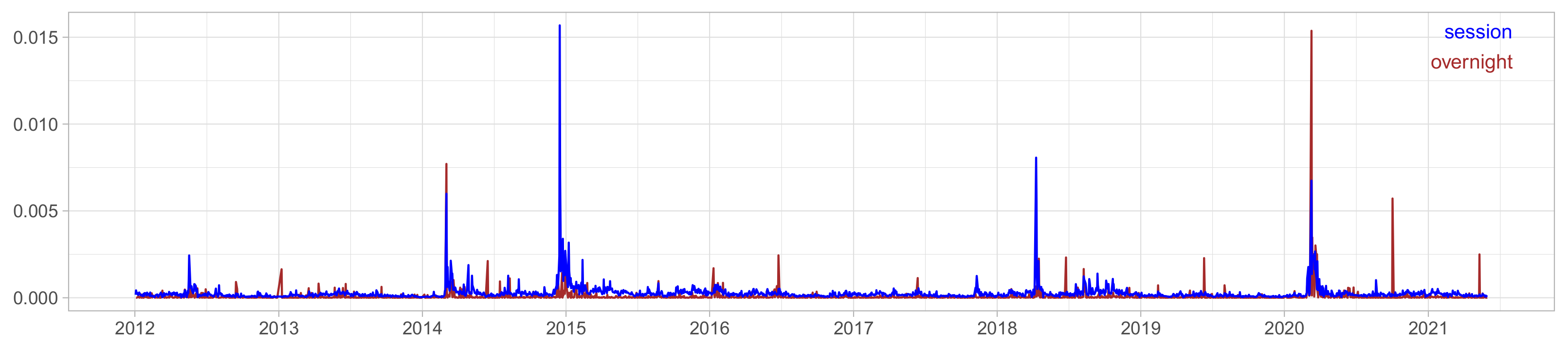
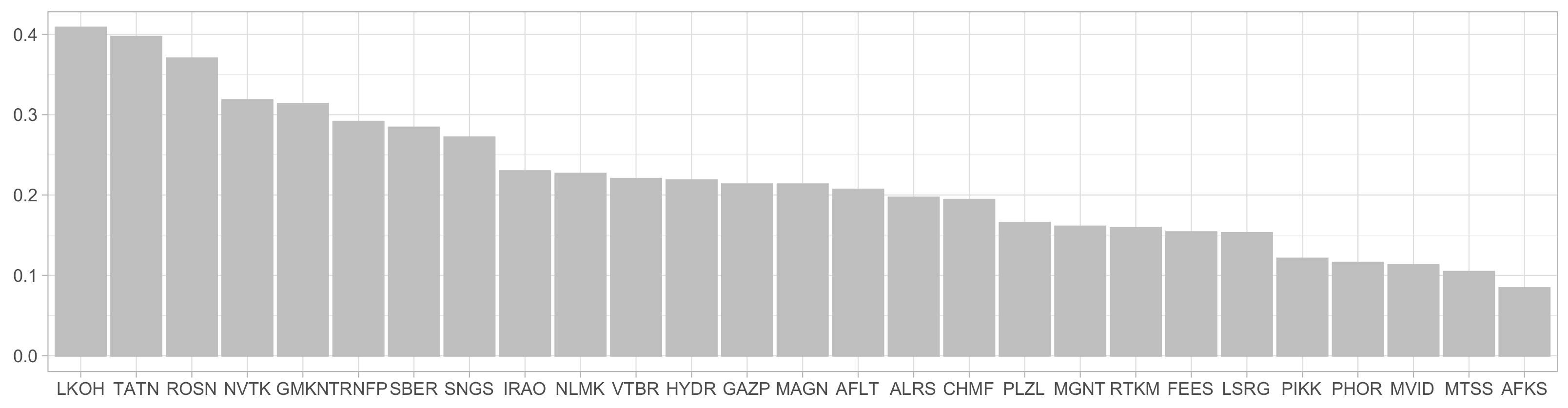
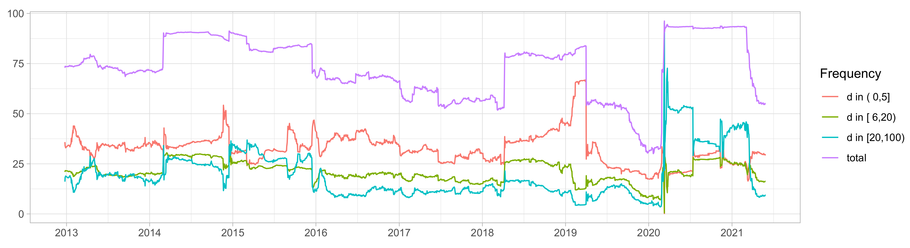
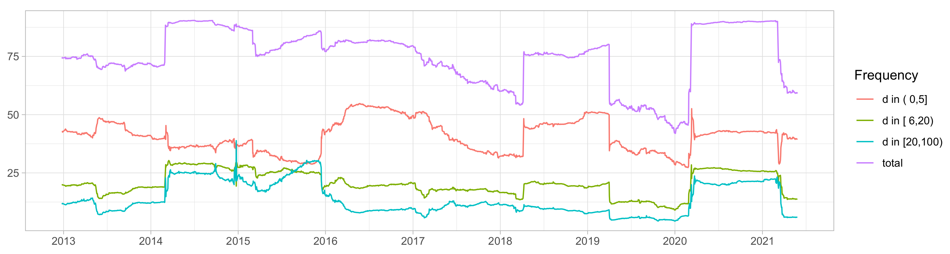
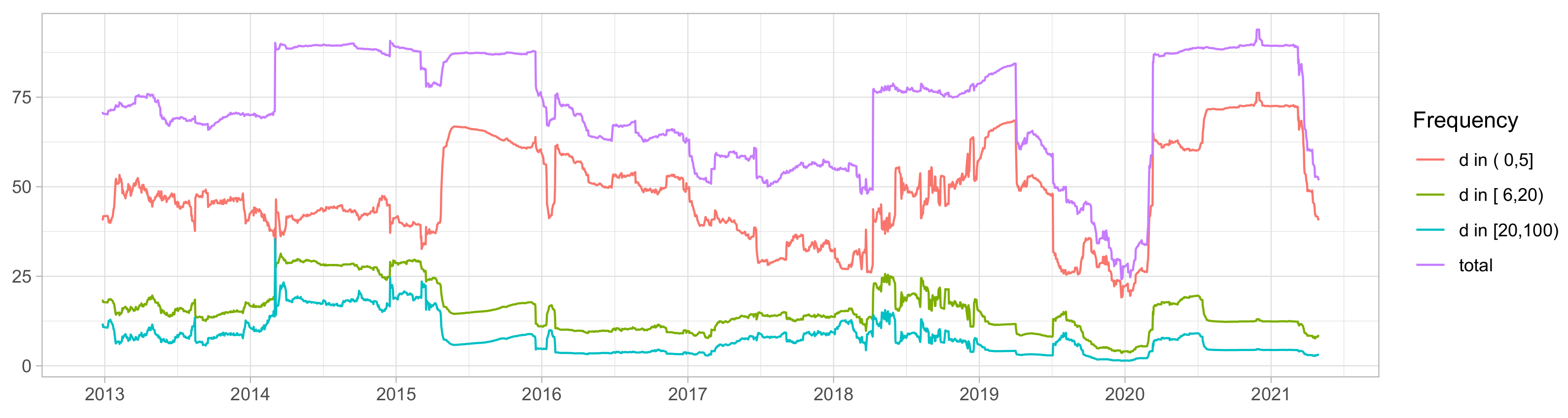

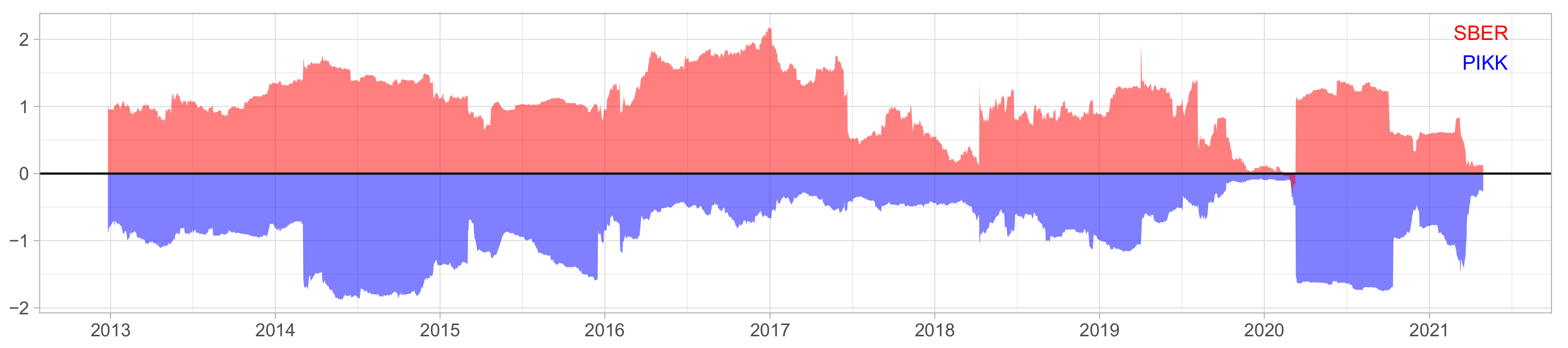
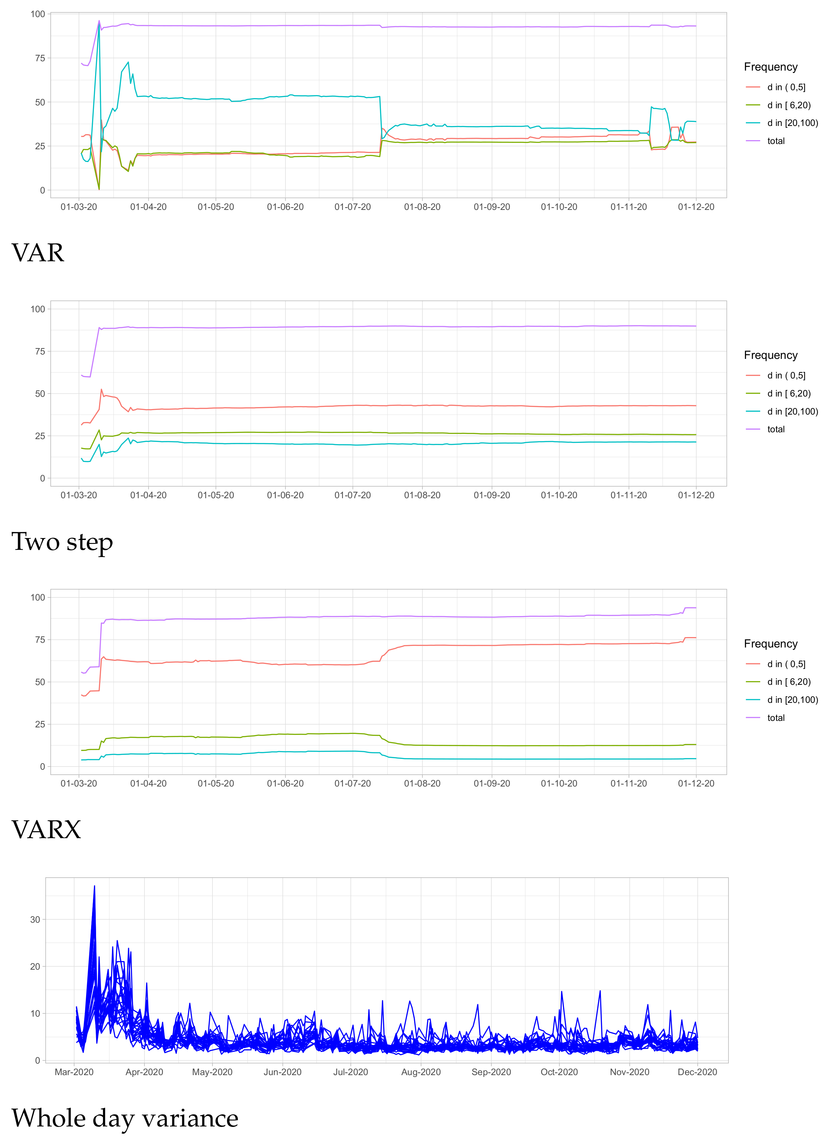
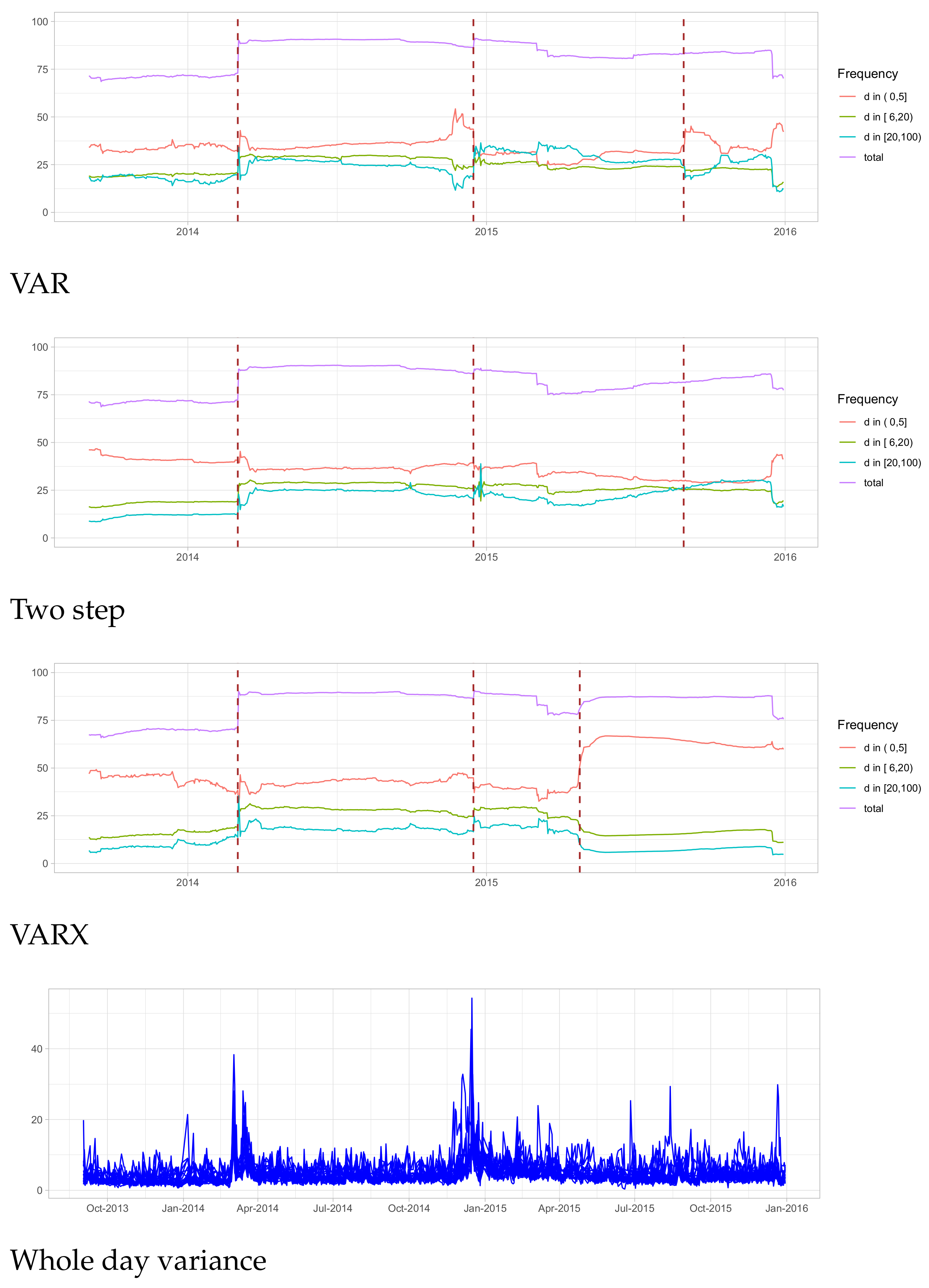
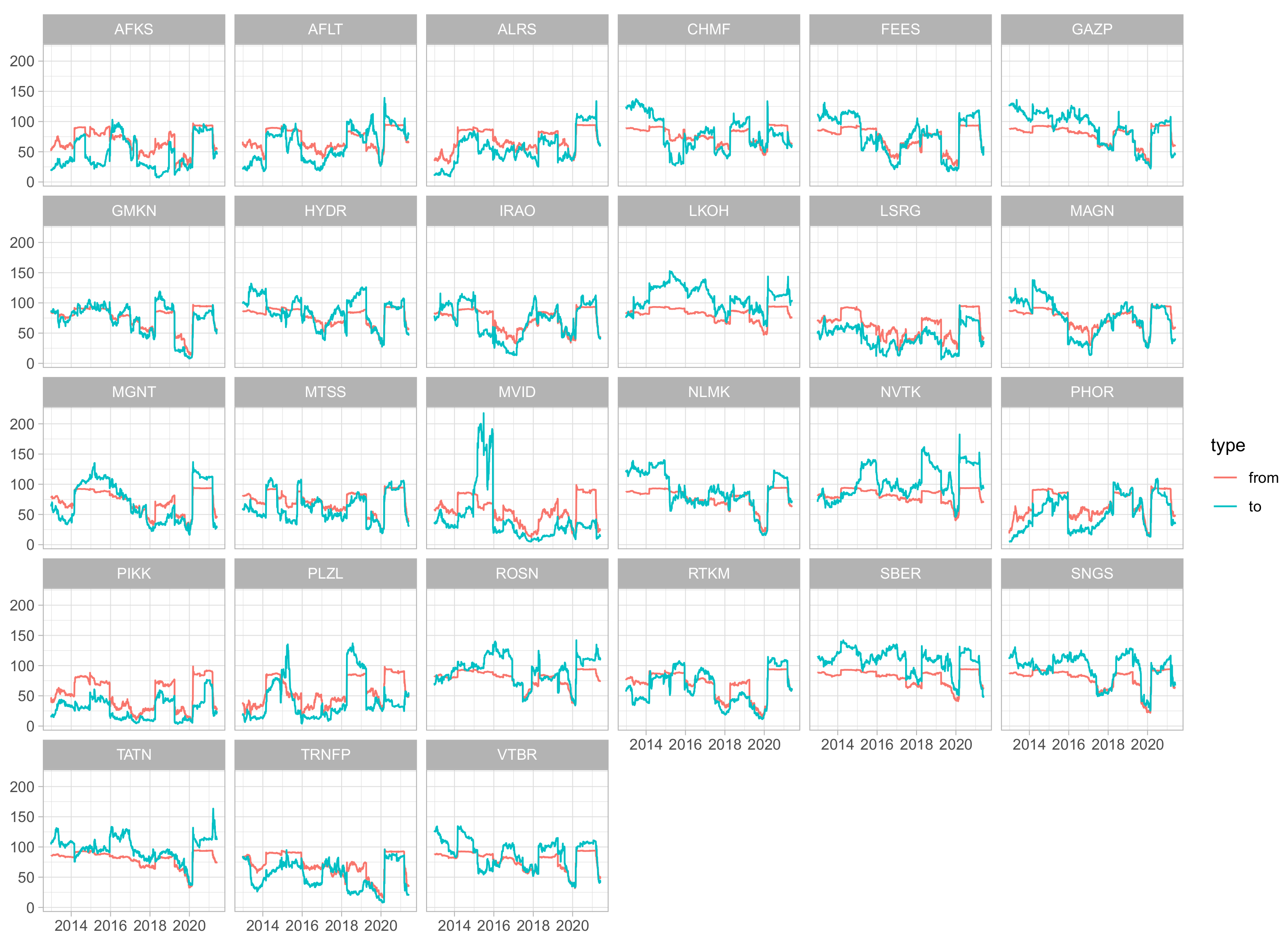
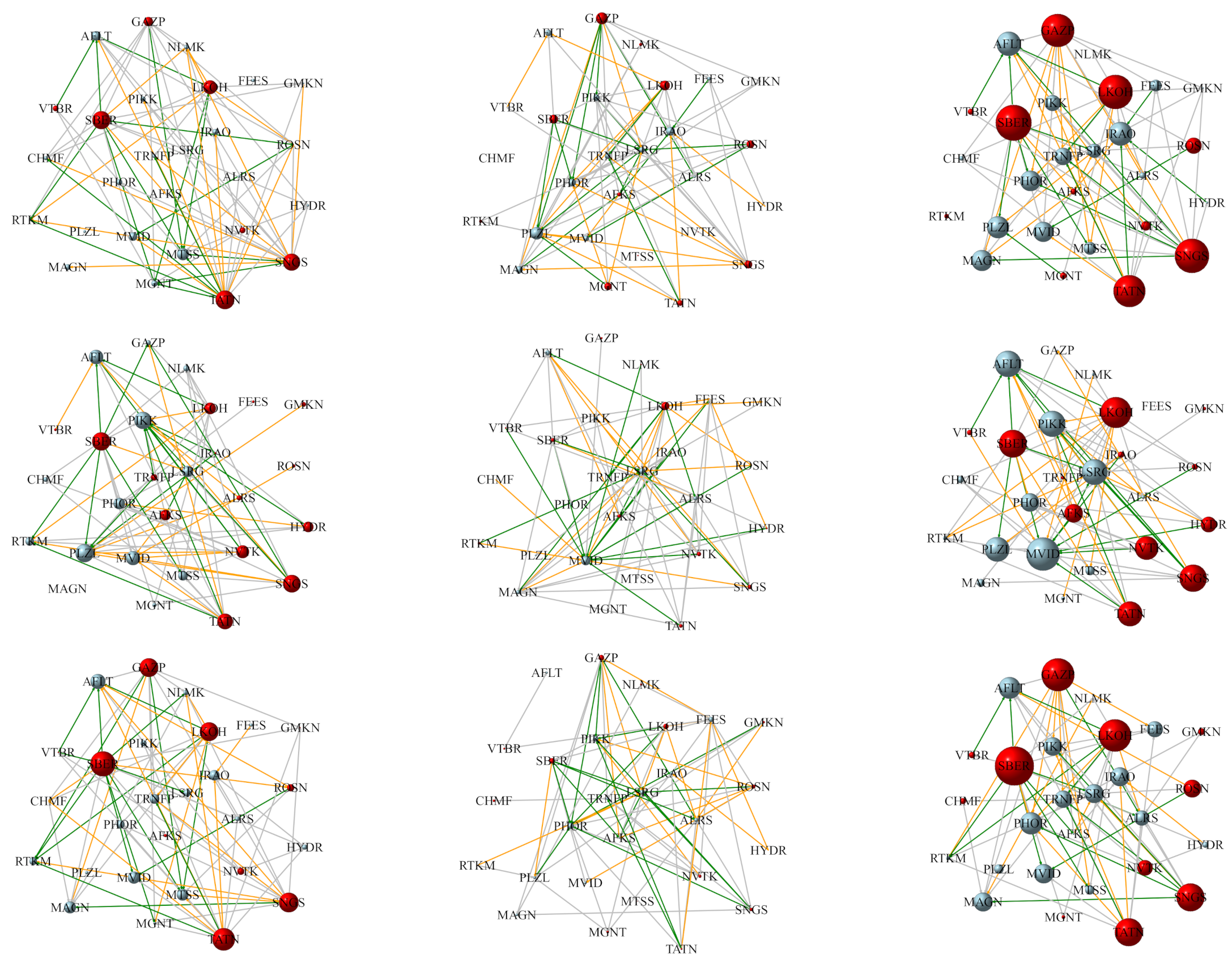
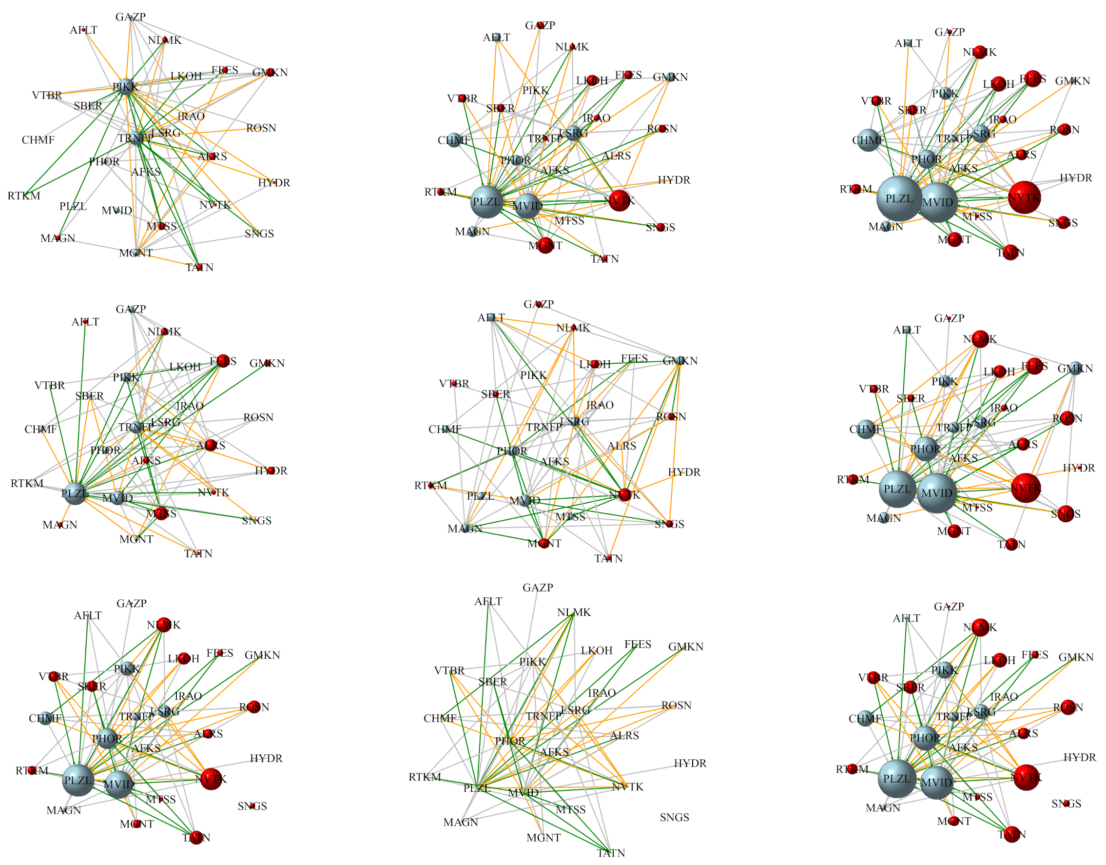
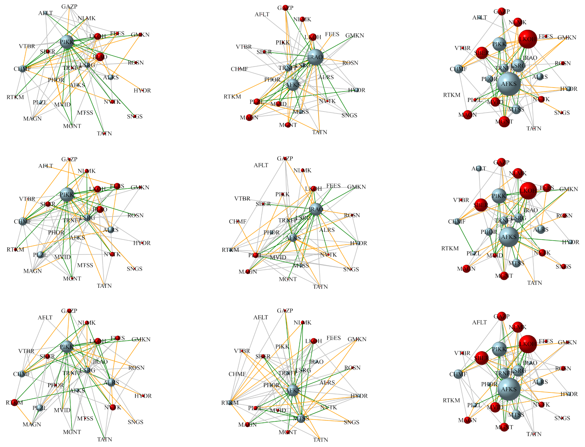
Publisher’s Note: MDPI stays neutral with regard to jurisdictional claims in published maps and institutional affiliations. |
© 2021 by the authors. Licensee MDPI, Basel, Switzerland. This article is an open access article distributed under the terms and conditions of the Creative Commons Attribution (CC BY) license (https://creativecommons.org/licenses/by/4.0/).