Abstract
In the present paper, we test the use of Markov-Switching (MS) models with time-fixed or Generalized Autoregressive Conditional Heteroskedasticity (GARCH) variances. This, to enhance the performance of a U.S. dollar-based portfolio that invest in the S&P 500 (SP500) stock index, the 3-month U.S. Treasury-bill (T-BILL) or the 1-month volatility index (VIX) futures. For the investment algorithm, we propose the use of two and three-regime, Gaussian and t-Student, MS and MS-GARCH models. This is done to forecast the probability of high volatility episodes in the SP500 and to determine the investment level in each asset. To test the algorithm, we simulated 8 portfolios that invested in these three assets, in a weekly basis from 23 December 2005 to 14 August 2020. Our results suggest that the use of MS and MS-GARCH models and VIX futures leads the simulated portfolio to outperform a buy and hold strategy in the SP500. Also, we found that this result holds only in high and extreme volatility periods. As a recommendation for practitioners, we found that our investment algorithm must be used only by institutional investors, given the impact of stock trading fees.
1. Introduction
Market volatility is a fundamental concept in Finance theory. This, by the fact that the main rationale of financial asset pricing estates that the higher the risk, the higher the reward (return or risk premia from a “risk-free” asset). We are not going to discuss this issue by the fact that Classical Finance theory and Behavioral Finance or Neurofinance probed as true this relationship.
In the specific case of asset pricing, the first proper mathematical modeling of investor’s rational selection comes from Markowitz [1,2,3], Roy [4], Tobin [5]. All these works, among other related ones, set the risk level (systemic or market risk level) as the key factor to determine the price of a given security. More specifically and following the seminal proposal of Markowitz, the risk level or volatility uses a as a proxy the standard deviation or the variance (), given an Expected return (). Departing from this, the rational selection of a given investor is made through a utility function . There are several proposed functional forms for this function of preferences. Despite this, the most used in the investment industry is the quadratic utility function of a security return (), proxied with a second order Taylor expansion around the expected return as constant:
As noted in (1), the personal and rational investment level () in a risky asset is determined by a personal risk aversion level (), its expected return and volatility () values. This leads to the next optimal investment level , given the interest rate of a “risk-free” asset ():
Departing from the previous asset pricing methods, the works of Samuelson [6,7] present a first effort, based in the previous work of Luis Bachellier, to model the behavior of the stochastic process of stock prices as risky assets. This is done to develop a model of the expected future price of stocks in stock options.
At that time, the proper mathematical model for pricing agricultural and stock options was a pending task since their historical inception in the ancient Greece. Departing from Samuelson’s work [8], Black & Scholes [9] and Merton [10] developed a model for the valuation of European security options that became the corner stone of the Chicago Board of options Exchange (CBOE); a market that is a subsidiary of the Chicago Mercantile Exchange (CME).
In their proposal, Black, Scholes and Merton arrived to the next put () and call () option valuation formulas, given a spot price () and a strike price ():
In the previous equations, is the Gaussian cumulative function that models the moneyness of the option, given the values and :
The moneyness probability of an option determines the value of the option, given the odds () that the option ends at the money ( in (3) or in (4)) or out of the money ( in (3) or in (4)) at time . This moneyness level depends, among the main factors, from the volatility or risk () level.
As noted from the asset pricing models in (1) to (6), the volatility level or risk exposure determines the proper price of a security or its optimal investment level. However, only in the last two decades, the risk level has been used as a hedging instrument or as a source of portfolio diversification.
Thanks to the work of Breeden and Litzenberger [11], the volatility level () can be estimated from (3) to (6) in a model-free context; by just observing the market price of put and call options with different strike prices (). Departing from this breakthrough, the implied option volatility level can be inferred from the outstanding options market price. This implied volatility level is assumed to be the same as the observed in the underlying asset [12].
Departing from the previous work, Brenner and Galai [13] proposed the development of a volatility index that can be estimated from the observed option market prices; this index that also could be used to hedge option risk. The rationale of their proposal is as follows: As noted from (3) to (6), the only market invariants (random variables that can be modeled with a defined and stable pdf) are:
- The spot price ( ), modelled with a log-normal pdf.
- The volatility ( ).
By assuming as “given” the spot price at the moment of option pricing (), the only random variable left is volatility (). If this volatility level increases, the option underwriter or holder could face important option price changes (losses). Therefore, the trader, hedger or issuer should be able to hedge not only the underlying spot price, but also the volatility level.
Departing from Brenner and Galai’s paper, the CME developed a group of indexes that measure the market volatility level, given the actual S&P 500 index put and call market prices. This index is known as the VIX (the acronym of Volatility IndeX). The first VIX version measured the observed volatility of options of the less diversified S&P 100 stock index options. Later, the CME changed the methodology to measure the market volatility of the S&P 500 index (henceforth SP500).
This index (VIX), as accepted in the investment industry [13,14,15], is a good proxy of the U.S. stock market risk level [12]. A level that is estimated from the future expectations of the S&P 500 index stock option traders. In Figure 1, we present the historical performance of the S&P 500 (blue line) and the VIX index (orange line).
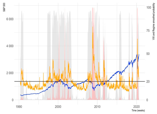
Figure 1.
The historical performance of the S&P 500 and VIX indexes. Color codes: The S&P 500 is depicted with a blue line, the VIX index with an orange one, the high volatility regime probability at t is the grey area and the “extreme” volatility regime is the red one. Source: Own elaboration with data from Refinitiv [16].
This index, as expected, is a good proxy of the U.S. stock market risk level. A risk level that is estimated from the future expectations of the SP500 index option traders. As noted by Standard and Poors in its VIX trading technical document [14], when the VIX index is above 20 (black horizontal line) the general volatility level in the SP500 is considered high.
Following Figure 1, when the VIX index increases its value above 20 and rises, the SP500 tends to fall. This means that the SP500 and the VIX have an inverse performance, being this relation a potential source of portfolio diversification. In the same figure, the reader can note the historical (smoothed) probability () of being in a “high” volatility regime () at (grey area) and the probability () of being in an “extreme volatility” (red area). As noted, when the probability of the high volatility was , the VIX tend to be above 20 and the SP500 tend to have a negative trend. Also, when , the SP500 showed an important fall in its level and the VIX an important jump in its value.
With this rationale, in 1993 the J.P. Morgan bank issued the first volatility (standard deviation) swap to the United Bank of Switzerland (UBS) [15]. A swap in which UBS made a fixed payment on exchange of a payment of GBP 1 million pounds per point of the implied volatility of options of the Financial Times Stock Exchange (FTSE) 100 index. The hedging goal was to cover the FTSE vega notional of UBS’ trading book. Vega is one of the sensitiveness metrics of an option’s value in (3) to (6). Is the first derivative of (3) or (4), given a change in the volatility () level. After this, several sporadic issues of volatility or variance swaps were made. After that, in 1998, the Deustcheterminbörse issued some of the first VIX futures of the Eurostoxx 50 index and, finally and by following Brenner and Galai’s [13] work, the CME start to trade VIX futures in 2003 [15]. A key issue of trading with volatility futures for diversification purposes is timing. That is because one of the main benefits of volatility derivatives is the possibility of adding value in the portfolio only in high volatility periods. Periods such as the 2008–2009 global financial crisis or the current 2020 COVID-19 financial and Economic distress period.
Departing from this, Figure 1 depicts the goal of the present paper. A VIX future could be an attractive security to hedge a U.S. dollar (USD) based stock portfolio. That is, the portfolio manager could buy a VIX future to compensate the SP500 (stock portfolio) extreme downward movements in a distress period. One drawback of this strategy is the fact that high volatility or distress time periods tend to be short-lived. Also, the proportion of time in which these episodes occur is smaller than the proportion of “normal” or low-volatility periods.
Another drawback of a VIX futures position is that the VIX future term structure has a monthly basis and, at redemption, an actual VIX future position must be rolled over. This carries roll-over costs by the fact that the longer-term VIX future position shows higher prices (a situation called “contango”).
To illustrate this, in Figure 2 we depict the historical performance of a 1-month S&P VIX short-term futures index [17]. This index started to trade at 20 December 2005 and proxies the performance of a “buy and hold” investment strategy in the 1-month or 2-month VIX futures. The performance of this index shows the impact that roll-over costs had.
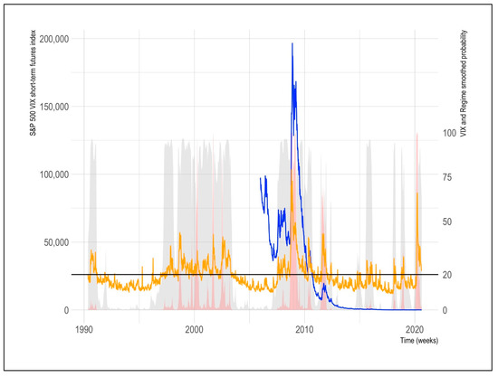
Figure 2.
The historical performance of the S&P 500 VIX short-term futures and VIX indexes. Color codes: The S&P 500 is depicted with a blue line, the VIX index with an orange one, the high volatility regime probability at t is the grey area and the “extreme” volatility regime is the red one. Source: Own elaboration with data from Refinitiv [16].
Despite these limitations, volatility futures are useful for volatility hedging purposes. By following Figure 2, the reader can note that the VIX futures had an important “jump” in periods when the probability of being in a “high” () or “extreme” () volatility regime was above 50% (grey and red areas). Given this, these futures could be used for diversification purposes if there is an appropriate method to enhance their timing. This is a conclusion widely discussed by several authors [15,18,19,20,21,22,23].
The smoothed regime probabilities of Figure 1 and Figure 2 were estimated with the use of a time series method know as Markov-Switching models [12,24,25,26,27] (MS).
By the fact that VIX futures could be an important diversification and risk hedging tool, we propose the use of MS models to determine the timing of VIX futures investing. More specifically, we propose the use of MS models, and their extension with Generalized Autoregressive Conditional Heteroskedaticity (MS-GARCH) variances [28,29,30,31]. This, to forecast the regime-specific smoothed probabilities ( at .
With these forecasts, we back tested a trading algorithm that simulated 8 portfolios diversified with the 1-month VIX futures (VIX), the SP500 stock index and the U.S. 3-month Treasury bills (T-BILL)
The hypothesis that we tested is that “the use of MS or MS-GARCH models for VIX futures diversification purposes, leads to an overperformance of the simulated portfolio against a buy and hold strategy”.
The main practical motivation of our test is the need of a proper timing method for volatility trading, along with the need of a proper quantitative method to determine the optimal VIX futures investment level in a portfolio. Nowadays there is a lack of well-known quantitative methods that could help investors to actively manage their VIX/equity portfolio positions.
The potential use of our test is the development of exchange traded funds (ETF) or other Publicly traded securities that could use our simulated VIX futures management algorithm. Securities like these could provide the benefit of investing more (less) in stocks during calm (distress) time periods and invest less (more) in VIX futures in distress (calm) ones. This, for the individual investor.
Also, the potential application of our investment algorithm could be of use for Institutional investors such as pension funds, insurance companies or Sovereign funds. This type of investor could have a proper timing technique to enhance their stock component in their portfolio and to preserve (or increase) its value during high volatility episodes. A highly discussed result is the fact that high volatility episodes have a significant negative impact in the asset value of this type of investor. This could lead to a wider gap between their assets value and their contingent claims (liabilities). With the use of a proper VIX future management algorithm this high volatility episodes could be value generating ones.
In a similar perspective, the theoretical motivation of our test is to enhance the scant discussion about the benefits of VIX futures trading and the use of these in portfolio management. As noted, the development of volatility derivatives is a recent topic in the Finance industry and could be a very promising practice in the future. This is done to have a better portfolio diversification in distress time periods. Also, these derivatives could be of use to hedge the loss of value of individual and Institutional investors. We hope, with our results, to enhance the discussion about these benefits and to prove the practical use of our investment algorithm.
Once our paper’s hypothesis has been presented, we structured our paper as follows: in the next section we make a brief literature review about VIX futures trading and the use of VIX futures and MS models in investment decisions. This, in order to show our theoretical motivations and to highlight the research gaps that we want to fill herein. In the third section we describe how did we gathered and processed the data, along with the observed results in our simulations. Finally, in the fourth section, we present our concluding remarks and suggestions for further research.
2. Literature Review
Volatility trading is a recent practice with scant literature review. Given this, several questions had to be solved first, in order to make a proper valuation and use of these derivatives. The first issue is the definition of volatility’s stochastic process. As it is known, the range of values of this parameter is . Also, an important feature of variance is that its value has a mean-reverting stochastic process.
In order to solve this, Grünbichler and Longstaff [32] developed the conditions of the stochastic process given in (7). In essence, this model has the same mean reverting properties of the Cox Ingersoll and Ross [33] and Longstaff and Schwarz volatility and interest rate option valuation models [34,35]. Given this, Grünbichler and Longstaff proposed the next stochastic process for the volatility:
A process in which is the variance level at (VIX index at ) and is the long-term mean-reverting variance value. is usually a value set to equal to zero the future payoffs of several VIX options with different strike prices. Also, in (7), is the rate at which revert to , is the volatility of the volatility and is a Wiener process.
These four works [32,33,34,35] developed the mathematical foundations of variance derivatives pricing models. Models that allowed a more liquid market for VIX futures markets. Also, these works were an important contribution to the market of variance swaps. More specifically, for valuation purposes and the determination of a long-term or strike value of the variance ().
Following these works, Dueker [12] compared the observed volatility values of the SP500 by using MS-GARCH models. More specifically the ones of Cai [36], Hamilton and Susmel [28], Hansen [37] and a single-regime GARCH model. This test was made with daily VIX and SP500 data from January 1986 to September 1994. In this work, the author found that the t-Student MS-GARCH model with time-varying kurtosis is the one that best fit the observed VIX values. A conclusion similar to the results observed herein. Also, the author concludes that, given the mean-reverting nature of the variance at , the VIX values show some extreme jumps when the regime in the SP500 market changes from to . He also found that these jumps tend to return to lower VIX values.
A similar conclusion to the previous one is the one given by Bakshi and Kappadia [38]. These two authors model the volatility (VIX) risk premium and gave strong proofs about the limitations of VIX futures as trading tool. This is because, given the roll-over cost, there is a fast mean-reverting feature of volatility and the related risk premium is negative. This result is the main motivation of the use of MS and MS-GARCH models for VIX future trading timing.
Given these works, several research efforts have been made, in order to develop proper VIX prediction models. From a future-spot relationship perspective, Zhang, Shu and Brenner [39], determine if the VIX future value correspond to the spot index value. They also studied the slope of the mean VIX future prices, against the spot ones. The authors found that the mean VIX future price is a good proxy to determine the fair value of VIX option prices. This is true, if a mean reverting model such as the one of Grünbichler and Longstaff [32], is assumed in “normal” (low volatility or ) market situations. A result that also motivates the use of MS models for VIX timing.
Later, Baba and Sakurai [40] tested the use of several U.S. macroeconomic variables as indicators or factors to forecast the VIX. This, in a three-regime context: “tranquil” or low volatility (), “turmoil” or high volatility () and “crisis” or extreme volatility (). With VIX monthly data from January 1990 to June 2010, the authors found appropriate the use of a 3-regime model. As a conclusion that motivates the test of using two and three regimes in the present paper. The authors also found that the shift from the tranquil () to the turmoil () regime can be forecasted with the U.S. rate lower term spreads (5-year U.S. T-Note rate minus the 3-month T-bill).
In a similar fashion, Romo [41] used two-regime MS and MS-GARCH models of the VIX time series to predict this index’s value. The author proved that it is appropriate the use of these models for trading purposes. This result also motivates our test of using these models for trading timing in this paper.
By performing a similar test in the Korean VIX index (VKOSPI), Song, Ryu and Webb [42] tested the use of several exogenous variables to model the performance of this volatility index; in a three-regime MS and MS-GARCH context. In their results, the authors found that the influence of U.S. financial variables is bigger than the Korean ones.
In a similar fashion, Chittineni [43] test the integration level of 6 VIX indexes (The Indian IVIX, the U.S. VIX, the Japanese VXJ, the German VDAX, the European Vstoxx and the Hong Kong VHSI). The author found, with daily data from 2 March 2002 to 30 December 20016, that only the U.S. and Hong Kong VIX indexes have an important correlation with the Indian IVIX during the high volatility () regime.
In a first news sentiment study, Shaikh [44] test the influence that the Economic Policy Uncertainty Index (EPUI) of Baker, Bloom and Davis [45] has in the performance of the VIX index. The EPUI is a news sentiment index estimated for several countries (including the U.S.) and this author find, with a two-regime MS model, that the EPUI has an important and direct influence in the VIX value; as a useful conclusion for the present paper for trading decisions.
Finally, in a VIX modeling and description perspective, the work of Fassas and Sinopoulos [46] makes a review of the 47 VIX indexes (for stocks and commodities in several countries) and observes that the relation between the spot price and the implied volatility behaves differently in commodities, currencies and stocks. As a result, the present paper that contemplates VIX futures as a diversification tool in portfolio management.
Some other works make a review of VIX modeling for option and derivatives valuation [47,48,49] but our main focus is the use of VIX futures for performance enhancement in portfolio management. As a departing point of this use, we found the work of Bondarenko [50] who studied the performance of U.S. hedge funds and found a causal relationship between their performance and their variance risk. Also, he found a potential return generation with the “sell” of variance risk. In a similar fashion, Dash and Moran [51] found evidence that the correlation between market volatility (VIX) and the performance of hedge funds is inverse and asymmetric.
Among the works who tested the benefits of VIX diversification, we found the work of Szado [18] who test the inverse relation of VIX futures in hedge funds during distress time periods. Daigler and Rossi [52] perform a mean-variance portfolio selection test between the SP500 and the VIX and show that the mean-variance profile increases importantly; this, given the observable negative correlation between VIX and SP500 stocks. As a result that motivates our test in a Markov-Switching context.
In a similar motivation, Hafner and Wallmeier [53] test the benefits of adding variance swaps of the DAX and the Eurostoxx 50 indexes. In their results, the authors found the benefits of a “option-like” return in their simulated portfolios.
In a similar mean-variance portfolio selection perspective with the use of the Black-Litterman [54] method and with skewness preference, Alexander, Kapraun and Korovilas [19,23] found no evidence in favor of VIX diversification in a SP500 portfolio. In an ex-ante perspective, Black-Litterman [54] portfolios tend to be optimal. But, in an ex-post or back test one, the simulated portfolio does not outperform a “pure stock portfolio”. This work was later extended by the same authors who made a similar study in the U.S. and European stock markets and found (as the previous work) that roll-over costs have an important impact in portfolio performance. They also found that only volatility diversification is beneficial during distress time periods. This last result is in line with ours, along with their conclusions of the benefits of this strategy in distress market periods.
We propose to use MS models to forecast the high () and extreme () volatility episodes. This, in order to determine if it’s appropriate to invest in VIX futures at .
With different conclusions, Fallon, Park and Ju [22] and Jung [55] found evidence in favor of portfolio diversification with more specific non mean-variance portfolio selection models. Also, these works motivate the present work by the fact that we want to use MS and MS-GARCH models for portfolio design. This without the consideration of correlations between assets and given the expected probabilities of each regime of the SP500 at as independent variables.
The use of MS models for investment decisions comes from the proposal of Brooks and Persand [56]. These authors estimated the Yield/dividend ratio of the 10-year U.K. Gilts and the FTSE 100 stock index.
By using a Gaussian two-regime MS model in this ratio, the authors developed a trading rule in which the investment level in the FTSE 100 () and the Gilt () depend on the smoothed regime-specific probability ():
By simulating a portfolio with monthly data from January 1975 to August 1997 for fitting, the authors made a back-test for the September 1980 to August 1997 period. The authors found that the trading strategy improves the mean-variance efficiency and performance of the simulated portfolio. This, against a “buy and hold” or “passive” one in stocks or Gilts.
MS and MS-GARCH models have been used for several purposes, such as the characterization of stock indexes, currencies or commodities’ time series [57,58,59,60,61,62,63,64,65,66,67,68,69,70]. The use of these models for the aforementioned has had also interesting extensions in Fuzzy logic and control applications [71,72].
Departing from Brooks and Persand’s work, some other extensions about their use in investment decisions have been tested.
Hang and Bekaert [73,74,75] developed a MS mean-variance framework in a multi asset portfolio. In their test with interest rates or the main equity benchmarks of the U.S., the U.K. and Germany, the authors found the benefits of a portfolio optimally selected with MS covariances; against the performance of the individual indexes.
Kritzman, Page and Turkington [76] simulated a U.S. dollar (USD) based multi-asset portfolio. A portfolio in which they tested the use of MS models to predict the likelihood of a high volatility episode in stocks, currencies, inflation and Economic growth. Given these smoothed probabilities, the authors suggested some “tilts” or marginal changes in each asset position. By using the Baum and Welsh [77] algorithm to estimate the MS models, the authors found that their simulated portfolio had a better performance than a static multi-asset portfolio.
In a similar fashion Hauptman et al. [78] and Engel, Wahl and Zagst [79] used three-regime MS models and several financial and Economic variables to develop a warning system in U.S., European and Japanese stocks. With this Economic and financial variables, the authors estimated time-varying smoothed regime probabilities and also time-varying transition probabilities (as in Filardo [80]). Given the use of exogenous variables for smoothed probability estimation, the authors proved the performance benefits in a stock-bonds portfolio. The conclusions of these authors are similar to the ones of the previous works, in the sense that MS models are useful for trading decisions (timing) in stock markets.
Another extensions to the tests of MS models in portfolio management are the one of De la Torre-Torres, Galeana-Figueroa and Álvarez-García [81]. These authors tested the use of MS-GARCH models in trading decisions in three of the main Latin American stock markets (Brazil, Chile and Mexico). By using two-regime, Gaussian, t-Student and Generalized Error Distribution likelihood functions, the authors tested the use of MS and MS-GARCH models in the next trading decision rule:
- (1)
- to invest in the simulated stock index if or.
- (2)
- to invest in the local risk-free asset otherwise.
Their results prove that the use of Gaussian MS-GARCH models leads to better performance (against a buy and hold strategy in stocks) in Brazil. This, with weekly data from 1998 to February 2019 and a simulation period from January 200 to February 2019. Also, they found that the use of t-Student MS-GARCH models leads to a similar conclusion in the Chilean market and the Gaussian MS one (non GARCH or time-fixed variance) in Mexico. This paper extends the review of the use of MS models to other stock markets, similarly to [82].
For the specific case of trading decisions in energy futures, we found the work of De la Torre-Torres, Galeana-Figueroa and Álvarez-García [83] who tested the use of MS and MS-GARCH models in the Oil and Natural gas markets. By using the 1-month contract weekly historic data of each commodity future, the authors simulated a portfolio that used the aforementioned investment strategy from June 1998 to February 2019 and found that only the use of a Gaussian MS model leads to an overperformance in the oil market. This, also against a buy and hold strategy in this commodity.
In a parallel perspective, Alizadeh, Nomikos and Puliassis [84] used MS-GARCH models to determine the proper Hedge ratio in Oil position, finding useful these models for the purposes tested.
Finally in the Agricultural futures markets, we can mention the works of Valera and Lee [67], De la Torre-Torres, Aguilasocho-Montoya and Del Río-Rama [85] and De la Torre-Torres et al. [86]. These works test the benefits of MS and MS-GARCH models in commodity spot prices and futures. The two last works tested the use of MS-GARCH models in the previous trading strategy in corn, soybean, cocoa and sugar futures. In their simulations, the authors found evidence that favors the use of MS and MS-GARCH models in these commodities. This, by the fact that use of MS-GARCH models in investment decisions also leads to a better portfolio performance.
As noted from the previous literature review and as stated in the previous section, MS and MS-GARCH models have been used only to forecast volatility or volatility index values in a given stock index options market. For the specific case of their use in volatility futures markets, nothing has been written. Departing from this, we want to fill this gap by testing a trading algorithm that invests in U.S. stocks (SP500 index), volatility (1-month VIX futures) and a risk-free asset (the U.S. 3-month Treasury-bill-TBILL-). This given the smoothed probability of a high () or extreme () volatility regime at .
Also, as noted in this literature review, VIX futures are a potential source of diversification. The main limitations of this approach are the roll-over cost and the fast mean-reverting property of variance. These are limitations that suggest the need of a proper timing method in these futures.
Our position in this paper is that the best way to diversify a portfolio with volatility is by making active management through an investment algorithm that uses MS or MS-GARCH for regime forecasting. The use of this algorithm leads to a better performance than a buy and hold SP500 only position.
Once we have presented the practical and theoretical motivations of our test, we will proceed to describe how did we gathered the input data and how did we perform our investment algorithm’s simulations.
3. Methodology: Data Gathering, Investment Decision Algorithm and Simulation Parameters
In order to simulate our investment strategy with MS or MS-GARCH models, we assumed that the SP500 could be modeled with a two or three-regime stochastic process. This, with a Gaussian or t-Student pdf as follows:
In our simulations, we estimated, at , the MS models in (9) and (10). We did this with either time-fixed, ARCH [87] or GARCH [88] variances as follows respectively:
In the previous expressions, is the continuous time weekly return (percentage variation) of the SP500 index level and are the residuals or differences of each return against its mean. As noted in (11) and given the estimation process of the MS-ARCH and MS-GARCH models, we will estimate the MS models from the residuals. This means that we estimated a stochastic process with only a scale (standard deviation) regime-switching parameter. This is done to achieve a more stable and feasible solution in the estimation method [28,29,30,31].
The MS (time-fixed variance), MS-ARCH and MS-GARCH models were estimated by using the Metropolis-Hastings [89,90] algorithm. This is a Bayesian estimation method that uses Monte Carlo simulations of Markov Chain.
From a weekly period from 23 December 2005 to 14 August 2020 (a total of 765 observations), we estimated two and three MS, MS-ARCH and MS-GARCH models in the SP500 index, with each pdf function in (9) and (10) and a variance model from (11) to (13).
For model estimation purposes, we used the weekly historical return data of the SP500 index from 6 January 6 1928 to the simulated week (). Given the estimation of the 8 MS, MS-ARCH or MS-GARCH models, we used the Deviance Information Criterion (DIC) [91] to determine which model is the most appropriate or best fitting.
Once that the best model was determined with the DIC, we made the regime specific smoothed probability forecasts at with the next expression:
As noted, we used the transition probability matrix and a vector of the last realizations of each regime-specific smoothed probability at time . We estimated the forecast given in (14) in a two and three-regime context, given the DIC value.
With these forecasted smoothed probabilities we determined the investment level () in each asset as in Brooks and Persand [56]. We did this for two or three regimes respectively:
We used this weighting method in order to extend the tests of Brière, Burges and Signori [92] and Alexander, Korovilas and Kapraun [19] in a Markov-Switching context.
As previously mentioned, our investment algorithm with MS or MS-GARCH models set aside the correlation between the SP500 and the VIX (contrary to Alexander, Korovilas and Kapraun [19]). We are assuming that the value of the VIX index is a result of the implied volatility option traders’ expectations for the SP500. Given this, we are assuming that the regime change in the VIX index is related to the one of the SP500 [12]. Therefore, we estimated the MS and MS-GARCH models only for the SP500 and determined the proper investment level in each asset.
In order to determine in which asset to invest in each regime, we simulated the 8 portfolios that we detailed in Table 1. As noted, the first two portfolios assumed a three-regime context in (14) and (15). Portfolios 3 to 4 assumed a two-regime framework and portfolios 5 to 8 selected either a two or three-regime model, given the observed DIC at t. In these last 4 portfolios, we combine two or three-regime portfolio investment levels () in each asset.

Table 1.
The portfolio assets in each investment scenario.
With these steps, we executed the simulation process through the steps of Algorithm 1. This for portfolios 1 to 4.
| Algorithm 1 The Markov-Switching VIX investment algorithm’s pseudocode for the simulated portfolios. |
For week 1 to 765:
|
| End |
The previous algorithm was simulated in R by using the MSGARCH library [93] for the estimation of the MS and MS-GARCH models.
For the specific case of portfolios 5 to 8 in which the best fitting model could be either a two or a three-regime one, step 3 is different. Instead of estimating 6 MS models, we estimated 12 of these (6 for the two-regime case and 6 for the three-regime one).
Also, the 8 portfolios of Table 1 were simulated for three type of investors:
- A theoretical investor that pays no trading costs in the SP500 trades.
- An individual investor that pays a 0.1% plus 10% of Value Added Tax (VAT) for the SP500 traded amount.
- An Institutional investor that pays 0.83% trading fee plus VAT of the monthly traded amount in the SP500.
With these three types of investor, we simulated the impact that financial costs had in the portfolio.
For the specific case of the simulated VIX component we included the impact of roll-over costs. In all the portfolios we assumed that the simulated investor invests in the SP500 through a zero-tracking error exchange traded fund (ETF), in the TBILL through a mutual fund with management fees of zero and the VIX 1-month futures directly in the CME market with no other trading costs.
The simulated portfolios are U.S. dollar (USD) based one. The SP500, VIX and TBILL data were retrieved from the databases of Refinitiv [16]. For the specific case of the SP500 index, we retrieved the historical weekly data of the S&P 500 stock index (the Refinitiv Identification Code or RIC is SPX). For the 1-month VIX futures, we used the historical data of the continuation 1-month VIX futures in the Chicago Mercantile Exchange (RIC VXc1). Finally, for the U.S. Treasury-bill fund we used the base 100 value of a theoretical portfolio that invested in the weekly equivalent rate of the 3-month U.S. risk-free rate published in Refinitiv (RIC US3MT = RR).
The historical performance and accumulated return of these three assets is summarized in Table 2. As noted, The SP500 index had an accumulated return of 165.86% and the TBILL 18.32%. The specific case of the accumulated return of the VIX futures is circumstantial. This doesn’t mean that these futures, per se, are a value generating security. That is, at the moment of performing these simulations the VIX index was in a 23.29 level (returning from a historical maximum value of 61.54 on 20 March 2020). This, against a starting value of 12.12 on 23 December 2005. This circumstantial return is due to the high and extreme volatility regimes observed in the first half of 2020.
Table 2.
Statistical and performance summary of the three portfolio assets (figures in percentage).
Also as expected, the SP500 weekly mean return of 0.13% is higher than the one of the TBILL. In a similar fashion, it is of interest the standard deviation of the VIX (the volatility of the volatility). It is significantly higher than the one observed in the SP500. This gives a marginal proof to the conclusion that the volatility futures are good for diversification if a proper timing method is used [19,23]. Parallel to this, it is of interest the minimum return and 5% percentile of VIX futures. These values are lower than the ones of the SP500, an issue that points to the fast mean-reverting properties of the VIX [15,19,26,36] and, once again, the need of active management of VIX futures in a portfolio.
Once that we detailed the investment algorithm steps, and simulation parameters, we will proceed to the review of our main results and findings.
4. Simulations Results and Discussion
In order to make a proper review of our simulations results, we organized these given the three types of simulated of investors described in the previous sections.
In Table 3, we present a summary of the mean DIC observed in each of the 12 simulated MS models. Given these observed values, it is noted that the two-regime Gaussian GARCH, the two-regime t-Student GARCH and the three-regime t-Student MS models were the most used ones during the simulated weeks.
Table 3.
Mean DIC observed value for the simulated portfolios.
Given this, we found strong proofs about the execution of step 3 of Algorithm 1. That is, to estimate the 12 MS models in parallel to determine, at , the most appropriate for the smoothed probabilities forecast.
Given this finding we used these simulated smoothed probabilities forecasts of the 765 weeks and summarized, in Table 4 and Figure 3, the performance of the theoretical investor that pays no stock trading fees.
Table 4.
Performance of the 8 simulated portfolios for a theoretical investor that pays no stock trading fees and only future trading roll-over costs.
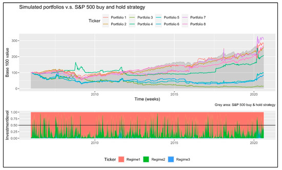
Figure 3.
The historical performance of the 8 simulated portfolios of a theoretical investor that pays VIX future roll-over costs and has no stock trading fees. Source: Own elaboration with data from Refinitiv [16].
As noted in Table 4, only the portfolios 1, 7 and 8 present an overperformance against the SP500 buy and hold strategy. By remembering Table 1, portfolio 1 invested more in the SP500 in low volatility periods () and in the VIX futures during the high ones (). Also, portfolio 7 had a combined strategy: if the appropriate number of regimes at is 2 (given the observed DIC values in step 3 of Algorithm 1), it followed the strategy of portfolio 1. But, if the appropriate number of regimes is 3, the simulated portfolios invested in the SP500 in low volatility periods (), in the TBILL in the high one () and in the VIX futures during extreme volatility episodes ().
The historical performance of portfolios 1 and 8 is depicted in the upper panel of Figure 3. This, as a red and pink line respectively. Also, the SP500 performance (buy and hold strategy) is shown with a grey area. In the lower panel of the same figure, we present the historical smoothed probabilities in a three-regime context. This lower panel allows us to present a reference of the expected regime at as investment level.
An interesting result of Figure 3 is the fact that, in the high () and extreme () volatility regimes, several portfolios (including 1 and 7) showed a jump in their value. As it is noted in the entire simulation, most of the portfolios underperformed the “buy and hold” SP500 strategy during calm times ().
For the specific case of Portfolios 1 (red line) and 4 (green line), these simulated portfolios showed an overperformance against the buy and hold strategy. This for the 9 September 2009 to 15 April 2011 period (in fact Portfolio 4 outperformed the buy and hold strategy in a wider period). As mentioned in Table 1, these two portfolios invested in VIX futures during or .
The potential reason of why, in the period 15 April 201 to 12 May 2017, the simulated portfolio underperformed the SP500, is the fact that this period is an Economic expansion one. Also, the volatility levels remained low (a VIX around or below 20). Given this, the simulated portfolios lagged in value, given the small investment levels that had in TBILLS or the VIX. Investment levels determined with (15) or (16) in step 5 of Algorithm 1.
In the period from 15 April 2001 to 12 May 2017, once again Portfolio 1 outperformed the buy and hold portfolio. This is explained by the fact that the U.S. had an electoral period in which the commercial and Economic policy uncertainty increased. This, given the trade and political position of the 2016–2020 U.S. elected president. This electoral period increased the volatility (VIX) levels and allowed Portfolios 1 and 8 to have a jump in their value. This situation allowed these two portfolios to outperform, once again, the buy and hold strategy.
From 9 February 2018 to 15 February 2019 period, the same U.S.-China trade tension increased once again the volatility in the stock markets. This allowed an increase of the values in the simulated portfolios. Also, the investment in VIX futures preserved the value of Portfolios 1 and 7 in this period. In the next low volatility weeks (22 February 2019 to 14 February 2020) the VIX value reverted to its mean value. Given this situation, the simulated portfolios reduced its position in these futures, but the current holdings lagged their value against the buy and hold strategy.
Finally, from 21 February 2020 to the end of our simulations, the COVID-19 pandemic episode sends the VIX value to record historical highs. This episode, as in the previously depicted ones, resulted in an increase in the probabilities of the high and extreme volatility. This also led to an increase in the VIX futures position and a jump in the value of Portfolios 1, 7 and 8. Given this, these portfolios outperformed, again, the buy and hold strategy.
From our simulations results, we want to highlight that the use of MS, MS-ARCH and MS-GARCH in a dynamic selection process (i.e., by means of the best fitting model through the DIC value) leads a good timing for VIX futures trading.
In our simulated portfolios (especially portfolios 1 and 7), the forecast of high volatility periods in the SP500 led to a proper forecast in the increase of volatility. Given this, the simulated algorithm could determine a higher investment level in VIX futures.
This result extends part of the recommendations made by Szado [18] and Brière, Burgues and Signori [92] by giving proofs that a dynamically managed portfolio with MS or MS-GARCH models could have a good diversification with stocks.
Unfortunately and in line with Alexander, Kapraun and Korovilas [19,23], this strategy is useful only in high or extreme volatility episodes. In the longer low volatility ones, our simulated portfolios tend to lag in value against the buy and hold strategy.
This result is in line with the concluding remarks of with Alexander, Kapraun and Korovilas [19,23]. This, by the fact that even if we present proofs that the use of MS or MS-GARCH models enhance VIX future trading in a stock portfolio, the timing improvements made need more review in order to solve the issue of a lagging performance of VIX diversification in low volatility periods.
In order to strengthen our review and to test if our trading algorithm is feasible in real life, we simulated the performance that an individual investor would have had, had she paid a 0.1% stock trading fee plus VAT. Our results are summarized in Table 5 and the historical performance of the simulated portfolios depicted in Figure 4.
Table 5.
Performance of the 8 simulated portfolios for a theoretical investor that pays no stock trading fees and future trading roll-over costs.
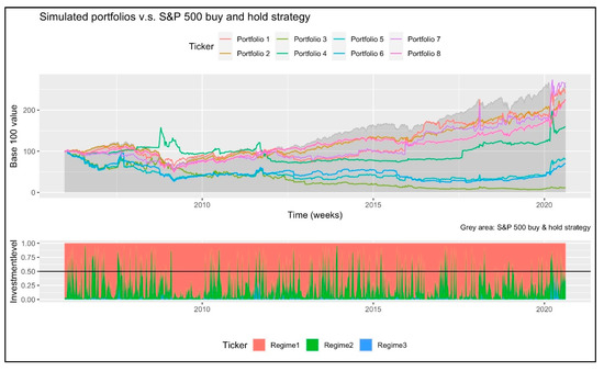
Figure 4.
The historical performance of the 8 simulated portfolios of an individual investor that pays VIX future roll-over costs and 0.1% stock trading fees plus VAT. Source: Own elaboration with data from Refinitiv [16].
For the specific case of an individual investor, to actively manage a stock portfolio with our strategy is not feasible. The stock trading costs erode the performance benefits. This, as expected and similar to Alexander, Kapraun and Korovilas [19,23]. Only in the specific case of the 2008–2009 financial crisis, the simulated portfolio outperformed the SP500. A result in line with the previously discussed literature about VIX diversification.
Finally, and in order to make a final test about our strategy’s feasibility, we present the performance results of a theoretical Institutional investor that pays a 1% yearly stock trading fee each month plus VAT. This, along with the potential roll-over costs in the VIX futures position.
In Table 6 we present the performance summary of this portfolio and, in Figure 5, the historical performance. As noted for this specific case, the stock trading and roll-over costs did not impact the performance of the simulated portfolio. In this simulated investor, Portfolio 1 paid a 168.68% accumulated return vs. the 176.09% achieved by the theoretical investor that paid no stock trading fees. In a similar analysis, Portfolio 7 earned a 196.32% in this scenario vs. de 206.64% of the theoretical investor. Finally, portfolio 8 paid to the simulated investor a 159.86% vs. a 170.16%.
Table 6.
Performance of the 8 simulated portfolios for a theoretical Institutional investor that pays a yearly 1% stock trading fee, in a monthly basis, and future trading roll-over costs.
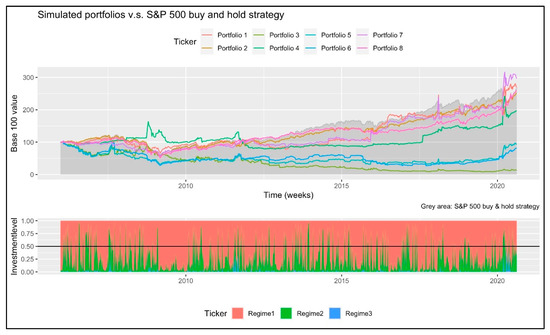
Figure 5.
The historical performance of the 8 simulated portfolios of an Institutional investor that pays VIX future roll-over costs and a monthly 0.83% stock trading fee plus VAT. Source: Own elaboration with data from Refinitiv [16].
These results are partly explained by the fact that the VIX position is actively managed (reducing the roll-over cost impact) and the burden of the stock trading costs is lower and paid with a lower frequency. Given this, the expected impact of stock trading costs is marginal and the results of the simulated portfolios for an institutional investor led to similar conclusions than the ones of the theoretical (stock fee-free) one.
As a corollary of our results and main findings, we can summarize that the use of MS or MS-GARCH models in an actively VIX futures-stocks portfolio led to a better VIX trading timing. Also, the benefits of using these models in a quantitative analysis tool, such as Algorithm 1, led to a proper portfolio diversification in distress time periods.
Despite these results, one limitation of this algorithm is the fact that a diversified portfolio in VIX futures led to a lagged performance against an SP500 buy and hold strategy; during low volatility periods.
Also, another drawback of the use Algorithm 1 is that it can only be used by institutional investors. If an individual investor carries out this strategy, the stock trading cost and taxes paid could lag her performance against a SP500 buy and hold strategy. Given this result, a potential suggestion for practitioners could be the development and management of an ETF that executes Algorithm 1. This security could potentially solve some of the risk premium drawbacks that the actual VIX ETFs and ETNs show. Also, it could provide a diversification option for individual investors.
5. Conclusions
The VIX index and its corresponding volatility futures are among the most recent, necessary and promising innovations in the investment industry [16,19,22]. This is so by the fact that these futures could provide a natural hedge in a stock portfolio in distressed time periods in financial markets.
Despite their potential use to enhance portfolio performance, to hedge the Vega notional of stock index options’ position or to profit with market volatility, these have some drawbacks. One is the fact that volatility (variance more specifically) is a fast mean-reverting variable [32,35]. That is, its stochastic process observes a long-term mean value. Even if the volatility level jumps, given the stock markets uncertainty [44], its value reverts fast [12,38].
Another limitation of diversifying a stock portfolio with VIX futures is the fact that the latter show a negative risk premium [15,19,22,26,36,39]. Also, in terms of time series analysis with Markov-Switching models, the high or extreme high volatility time periods tend to be short-lived.
Departing from the conclusions of Brière, Burgues and Signori [20], Alexander, Kapraun and Korovilas [19,23], Fallon, Park and Yu [22] and Jung [55], it is of practical need a proper timing method for volatility diversification. That means that the volatility portfolio diversification must be an active one, in which the volatility and stock positions must be rebalanced given the current market conditions.
A potential quantitative method that we tested for this purpose is Hamilton’s [24,25] filter; a time series method known also as Markov-Switching (MS) methods. We tested, for timing purposes, the use of this model and its extension with Generalized Autoregressive Conditional Heteroskedasticity (GARCH) variance [27,28] (or MS-GARCH).
MS and MS-GARCH models are Bayesian time series models in which the stochastic process of a given time series (such as the one of the S&P 500 or SP500 stock index) could be modeled in a number of regimes. For the purposes of the present paper, these were used to forecast (at ) a low volatility (), a high volatility () and an extreme volatility () regime at .
With the forecasted regime probabilities (), Brooks and Persand [56] suggest to determine the investment level () in a given asset. That is: . As an example: if a portfolio manager plans to invest in stocks in low volatility time periods () and in a risk free () asset in the distressed ones (), the investment level in each will be determined by the corresponding forecasted regime probability. This means: and .
With the use of two and three-regime MS and MS-GARCH models with Gaussian or t-Student likelihoods, along with time-fixed, ARCH or GARCH variances, we simulated 8 portfolios invested in the SP500, the VIX futures or the 3-month U.S. Treasury bills (T-BILL). We did this, with weekly simulations from 23 December 2005 to 14 August 2020 (a total of 765 weeks).
These 8 portfolios were simulated for 3 type of investors:
- A theoretical investor that pays roll-over costs in the VIX futures position and no stock trading fees.
- An individual investor that pays the roll-over costs and a 0.1% stock trading fee, plus a 10% of Value Added Tax (VAT).
- An Institutional investor that paid, in a monthly basis, a 1% yearly trading fee, plus VAT, in the monthly SP500 traded amount. This, along with the corresponding roll-over VIX futures costs.
For the case of the theoretical stock fee-free investor, we found that the simulated portfolios that diversified with VIX futures outperformed the SP500 buy and hold strategy; in high and extreme volatility periods. Also, at the end of our simulations, this portfolio showed a significant outperformance, given the pandemic extreme volatility episode of year 2020.
Our simulation results give proofs that MS and MS-GARCH models are suitable for VIX diversification timing, but these hold only in time periods in high or extreme volatility periods.
When we tested our VIX diversification algorithm with an individual investor that pays stock trading fees, we found it of no use. We conclude this by the fact that the stock trading fees erode the outperformance of the simulated portfolios. Given this, our simulated algorithm is not recommended for an individual investor that pays a stock trading fee of 0.1% (plus 10% of VAT) or more.
Finally, we tested our algorithm with an Institutional investor that pays a 0.83% monthly stock trading fee. In this case, we found similar results to the theoretical stock fee-free scenario. Given the access to more flexible trading fees, the impact of these were low.
With our results we conclude that the use of two or three MS and MS-GARCH models could be useful to enhance portfolio diversification with VIX futures. Also, and to allow a proper access of this strategy to individual investors, we suggest the development and management of Exchange Traded Funds (ETF) that could use our simulated algorithm as part of its investment policy.
As guideline for further research, we suggest testing this VIX investment strategy in different periodicities (daily or intraday), different likelihood functions or even asymmetric GARCH variances.
The estimation of MS or MS-GARCH models with time-varying transition probabilities (as in Filardo [80]) or the extension of the tests made by Alexander, Korovilas and Kapraun [19] in a Markov-Switching context could be also of potential interest.
In a parallel scope to the previous suggestion, the development of MS-GARCH models with heterogeneous periodicities (MS-MIDAS-GARCH) could be of interest. That is, to extend the estimation of volatilities with exogenous variables as in [94,95,96] to a MS context. This extension could be of use to estimate and to forecast more accurate smoothed probabilities for VIX trading decisions.
Finally, the use of MS-GARCH models in a fuzzy logic context could be also of interest as a potential extension. This by following [71,72], in order to reduce the impact of uncertainty effect from financial markets.
Author Contributions
Conceptualization, Data gathering, Simulations and Numerical Tests. O.V.D.l.T.-T.; Methodology, Formal Analysis, Investigation, Writing-Original Draft Preparation, O.V.D.l.T.-T., F.V.-M. and M.I.M.-T.-E. Writing-Review & Editing, F.V.-M. and M.I.M.-T.-E. All authors have read and agreed to the published version of the manuscript.
Funding
This research was funded by the Coordinación de la Investigación Científica at Universidad Michoacana de San Nicolás de Hidalgo and by the Instituto Politécnico Nacional.
Institutional Review Board Statement
Not applicable.
Informed Consent Statement
Not applicable.
Data Availability Statement
The simulation and test results data presented in this study are available on request from the corresponding author. The input data used herein is not publicly available, given the financial data base user agreement restrictions. The input data can be found in Public financial web sites.
Conflicts of Interest
The authors declare no conflict of interest in the tests and results presented herein. The funders had no role in the design of the study; in the collection, analyses, or interpretation of data; in the writing of the manuscript, or in the decision to publish the results.
References
- Markowitz, H. Portfolio selection. J. Finance 1952, 7, 77–91. [Google Scholar] [CrossRef]
- Markowitz, H. The optimization of quadratic functions subject to linear constraints. Nav. Res. Logist. Q. 1956, 3, 1–113. [Google Scholar] [CrossRef]
- Markowitz, H. Portfolio Selection. Efficient Diversification of Investments; Yale University Press: New Haven, CT, USA, 1959. [Google Scholar]
- Roy, A.D. Safety First and the Holding of Assets. Econometrica 1952, 20, 431. [Google Scholar] [CrossRef]
- Tobin, J. Liquidity preference as behavior toward risk. Rev. Econ. Stud. 1958, XXV, 65–86. [Google Scholar] [CrossRef]
- Samuelson, P. Proof that properly anticipated prices fluctuate randomly. Ind. Manag. Rev. 1965, 6, 41–49. [Google Scholar]
- Samuelson, P.A. Proof That Properly Discounted Present Values of Assets Vibrate Randomly. Bell J. Econ. Manag. Sci. 1973, 4, 369–374. [Google Scholar] [CrossRef]
- Black, F. Capital Market Equilibrium with Restricted Borrowingt. J. Bus. 1972, 45, 444–455. [Google Scholar] [CrossRef]
- Black, F.; Scholes, M. The Pricing of Options and Corporate Liabilities. J. Polit. Econ. 1973, 81, 637–654. [Google Scholar] [CrossRef]
- Merton, R.C. Theory of rational option pricing. Bell J Econ Manag. Sci 1973, 4, 141–183. [Google Scholar] [CrossRef]
- Breeden, D.T.; Litzenberger, R.H. Prices of state-contigent claims implicit in option prices. J. Bus. 1978, 51, 621–651. [Google Scholar] [CrossRef]
- Dueker, M.J. Markov Switching in GARCH Processes and Mean-Reverting Stock-Market Volatility. J. Bus. Econ. Stat. 1997, 15, 26–34. [Google Scholar] [CrossRef]
- Brenner, M.; Galai, D. New Financial Instruments for Hedge Changes in Volatility. Financ. Anal. J. 1989, 45, 61–65. [Google Scholar] [CrossRef]
- S&P Dow Jones Indices A Practitioners Guide to Reading VIX. Available online: https://cdn.cboe.com/resources/vix/SandP%20A%20Practitioners%20Guide%20to%20Reading%20VIX.pdf (accessed on 27 July 2020).
- Carr, P.; Lee, R. Volatility derivatives. Annu. Rev. Financ. Econ. 2009, 1, 319–339. [Google Scholar] [CrossRef]
- Refinitiv Refinitiv Eikon. Available online: https://eikon.thomsonreuters.com/index.html (accessed on 17 August 2020).
- S&P Dow Jones Indices LLC S&P 500 VIX Short-Term Index MCAP. Available online: https://www.spglobal.com/spdji/en/indices/strategy/sp-500-vix-short-term-index-mcap/# (accessed on 23 August 2020).
- Szado, E. VIX Futures and options: a case study of portfolio diversification during the 2008 financial crisis. J. Altern. Investments 2009, 12, 68–85. [Google Scholar] [CrossRef]
- Alexander, C.; Korovilas, D.; Kapraun, J. Diversification with volatility products. J. Int. Money Financ. 2016, 65, 213–235. [Google Scholar] [CrossRef]
- Brière, M.; Fermanian, J.-D.; Malongo, H.; Signori, O. Volatility Strategies for Global and Country Specific European Investors. Available online: https://papers.ssrn.com/sol3/papers.cfm?abstract_id=1945703 (accessed on 31 August 2020).
- Guobuzaite, R.; Martinelli, L. The Benefits of Volatility Derivatives in Equity Portfolio Management. Available online: https://risk.edhec.edu/publications/benefits-volatility-derivatives-equity-portfolio-management (accessed on 3 February 2019).
- Fallon, W.; Park, J.; Yu, D. Asset allocation implications of the global volatility premium. Financ. Anal. J. 2015, 71, 38–56. [Google Scholar] [CrossRef]
- Alexander, C.; Kapraun, J.; Korovilas, D. Trading and investing in volatility products. Financ. Mark. Inst. Instrum. 2015, 24, 313–347. [Google Scholar] [CrossRef]
- Hamilton, J.D. A new approach to the economic analysis of nonstationary time series and the business cycle. Econometrica 1989, 57, 357–384. [Google Scholar] [CrossRef]
- Hamilton, J.D. Analysis of time series subject to changes in regime. J. Econom. 1990, 45, 39–70. [Google Scholar] [CrossRef]
- Hamilton, J.D. Time Series Analysis; Princeton University Press: Princeton, NJ, USA, 1994. [Google Scholar]
- Haas, M.; Mittnik, S.; Paolella, M.S. Mixed normal conditional heteroskedasticity. J. Financ. Econom. 2004, 2, 211–250. [Google Scholar] [CrossRef]
- Hamilton, J.D.; Susmel, R. Autoregressive conditional heteroskedasticity and changes in regime. J. Econom. 1994, 64, 307–333. [Google Scholar] [CrossRef]
- Haas, M.; Mittnik, S.; Paolella, M.S. A new approach to Markov-Switching GARCH models. J. Financ. Econom. 2004, 2, 493–530. [Google Scholar] [CrossRef]
- Haas, M.; Krause, J.; Paolella, M.S.; Steude, S.C. Time-varying mixture GARCH models and asymmetric volatility. N. Am. J. Econ. Financ. 2013, 26, 602–623. [Google Scholar] [CrossRef]
- Ardia, D.; Bluteau, K.; Boudt, K.; Catania, L. Forecasting risk with Markov-switching GARCH models:A large-scale performance study. Int. J. Forecast. 2018, 34, 733–747. [Google Scholar] [CrossRef]
- Grünbichler, A.; Longstaff, F.A. Valuing futures and options on volatility. J. Bank. Financ. 1996, 20, 985–1001. [Google Scholar] [CrossRef]
- Cox, J.C.; Ingersoll, J.E.; Ross, S.A. A theory of the term structure of interest rates. Econometrica 1985, 53, 385–408. [Google Scholar] [CrossRef]
- Longstaff, F.A. The valuation of options on yields. J. Financ. Econ. 1990, 26, 97–121. [Google Scholar] [CrossRef]
- Longstaff, F.A.; Schwartz, E.S. Interest rate volatility and the term structure: a two-factor general equilibrium model. J. Finance 1992, 47, 1259. [Google Scholar] [CrossRef]
- Cai, J. A Markov model of Switching-Regime ARCH. J. Bus. Econ. Stat. 1994, 12, 309–316. [Google Scholar]
- Hansen, B.E. The Likelihood ratio test under non-standard conditions: testing the Markov Switching model of GNP. J. Appl. Econom. 1992, 7, S61–S82. [Google Scholar] [CrossRef]
- Bakshi, G.; Kapadia, N. Delta-Hedged gains and the negative market volatility risk premium. Rev. Financ. Stud. Summer 2003, 16, 527–566. [Google Scholar] [CrossRef]
- Zhang, J.E.; Shu, J.; Brenner, M. The new market for volatility trading. J. Futur. Mark. 2005, 30, 809–833. [Google Scholar] [CrossRef]
- Baba, N.; Sakurai, Y. Predicting regime switches in the VIX index with macroeconomic variables. Appl. Econ. Lett. 2011, 18, 1415–1419. [Google Scholar] [CrossRef]
- Romo, M. Volatility regimes for the VIX index. Rev. Econ. Apl. 2012, XX, 111–134. [Google Scholar]
- Song, W.; Ryu, D.; Webb, R.I. Overseas market shocks and VKOSPI dynamics: a Markov-switching approach. Financ. Res. Lett. 2016, 16, 275–282. [Google Scholar] [CrossRef]
- Chittineni, J. Regime switching behavior of indian VIX and its time dependent correlation with select developed economies. Bus. Econ. Horiz. 2017, 13, 666–675. [Google Scholar] [CrossRef]
- Shaikh, I. On the relationship between economic policy uncertainty and the implied volatility index. Sustainability 2019, 11, 1628. [Google Scholar] [CrossRef]
- Baker, S.R.; Bloom, N.; Davis, S.J. Measuring Economic Policy Uncertainty. Q. J. Econ. 2016, 131, 1593–1636. [Google Scholar] [CrossRef]
- Fassas, A.P.; Siriopoulos, C. Implied volatility indices—A review. Q. Rev. Econ. Financ. 2020. [Google Scholar] [CrossRef]
- Elliott, R.J.; Kuen Siu, T.; Chan, L. Pricing volatility swaps under Heston’s stochastic volatility model with regime switching. Appl. Math. Financ. 2007, 14, 41–62. [Google Scholar] [CrossRef]
- Aingworth, D.D.; Das, S.R.; Motwani, R. Quantitative Finance A simple approach for pricing equity options with Markov switching state variables A simple approach for pricing equity options with Markov switching state variables. Quant. Financ. 2006, 6, 95–105. [Google Scholar] [CrossRef]
- Papanicolaou, A.; Sircar, R. A regime-switching Heston model for VIX and S&P 500 implied volatilities. Quant. Financ. 2014, 14, 1811–1827. [Google Scholar] [CrossRef]
- Bondarenko, O. Market Price of Variance Risk and Performance of Hedge Funds. Available online: https://papers.ssrn.com/sol3/papers.cfm?abstract_id=542182 (accessed on 6 September 2020).
- Dash, S.; Moran, M.T. VIX as a companion for hedge fund portfolios. J. Altern. Invest. 2005, 8, 75–80. [Google Scholar] [CrossRef]
- Daigler, R.T.; Rossi, L. A Portfolio of stocks and volatility. J. Invest. 2006, 15, 99–106. [Google Scholar] [CrossRef]
- Hafner, R.; Wallmeier, M. Volatility as an asset class: European evidence. Eur. J. Financ. 2007, 13, 621–644. [Google Scholar] [CrossRef]
- Black, F.; Litterman, R. Global portfolio optimization. Financ. Anal. J. 1992, 48, 28–43. [Google Scholar] [CrossRef]
- Jung, Y.C. A portfolio insurance strategy for volatility index (VIX) futures. Q. Rev. Econ. Financ. 2016, 60, 189–200. [Google Scholar] [CrossRef]
- Brooks, C.; Persand, G. The trading profitability of forecasts of the gilt–equity yield ratio. Int. J. Forecast. 2001, 17, 11–29. [Google Scholar] [CrossRef]
- Klein, A.C. Time-variations in herding behavior: Evidence from a Markov switching SUR model. J. Int. Financ. Mark. Inst. Money 2013, 26, 291–304. [Google Scholar] [CrossRef]
- Areal, N.; Cortez, M.C.; Silva, F. The conditional performance of US mutual funds over different market regimes: Do different types of ethical screens matter? Financ. Mark. Portf. Manag. 2013, 27, 397–429. [Google Scholar] [CrossRef]
- Ardia, D.; Kolly, J.; Trottier, D.-A. The impact of parameter and model uncertainty on market risk predictions from GARCH-type models. J. Forecast. 2017, 36, 808–823. [Google Scholar] [CrossRef]
- Ardia, D.; Hoogerheide, L.F. GARCH models for daily stock returns: Impact of estimation frequency on Value-at-Risk and Expected Shortfall forecasts. Econ. Lett. 2014, 123, 187–190. [Google Scholar] [CrossRef]
- Ye, W.; Zhu, Y.; Wu, Y.; Miao, B. Markov regime-switching quantile regression models and financial contagion detection. Insur. Math. Econ. 2016, 67, 21–26. [Google Scholar] [CrossRef]
- Balcilar, M.; Demirer, R.; Gupta, R. Do sustainable stocks offer diversification benefits for conventional portfolios? An empirical analysis of risk spillovers and dynamic correlations. Sustainability 2017, 9, 1799. [Google Scholar] [CrossRef]
- Boamah, N.A.; Watts, E.J.; Loudon, G. Investigating temporal variation in the global and regional integration of African stock markets. J. Multinatl. Financ. Manag. 2016, 36, 103–118. [Google Scholar] [CrossRef]
- Bundoo, S.K. Stock market development and integration in SADC (Southern African Development Community). J. Adv. Res. 2017, 7, 64–72. [Google Scholar] [CrossRef]
- Ma, J.; Deng, X.; Ho, K.-C.; Tsai, S.-B. Regime-Switching Determinants for Spreads of Emerging Markets Sovereign Credit Default Swaps. Sustainability 2018, 10, 2730. [Google Scholar] [CrossRef]
- Zeitlberger, A.C.M.; Brauneis, A. Modeling carbon spot and futures price returns with GARCH and Markov switching GARCH models Evidence from the first commitment period (2008–2012). CEJOR 2016, 24, 149–176. [Google Scholar] [CrossRef]
- Valera, H.G.A.; Lee, J. Do rice prices follow a random walk? Evidence from Markov switching unit root tests for Asian markets. Agric. Econ. 2016, 47, 683–695. [Google Scholar] [CrossRef]
- Hou, C.; Nguyen, B.H. Understanding the US natural gas market: A Markov switching VAR approach. Energy Econ. 2018, 75, 42–53. [Google Scholar] [CrossRef]
- Balcilar, M.; van Eyden, R.; Uwilingiye, J.; Gupta, R. The Impact of Oil Price on South African GDP Growth: A Bayesian Markov Switching-VAR Analysis. African Dev. Rev. 2017, 29, 319–336. [Google Scholar] [CrossRef]
- Herrera, R.; Rodriguez, A.; Pino, G. Modeling and forecasting extreme commodity prices: A Markov-Switching based extreme value model. Energy Econ. 2017, 63, 129–143. [Google Scholar] [CrossRef]
- Kristjanpoller, W.R.; Michell, K.V. A stock market risk forecasting model through integration of switching regime, ANFIS and GARCH techniques. Appl. Soft Comput. J. 2018, 67, 106–116. [Google Scholar] [CrossRef]
- Falcone, P.M.; De Rosa, S.P. Use of fuzzy cognitive maps to develop policy strategies for the optimization of municipal waste management: A case study of the land of fires (Italy). Land Use Policy 2020, 96, 104680. [Google Scholar] [CrossRef]
- Ang, A.; Bekaert, G. Regime Switches in Interest Rates. J. Bus. Econ. Stat. 2002, 20, 163–182. [Google Scholar] [CrossRef]
- Ang, A.; Bekaert, G. How regimes affect asset allocation. Financ. Anal. J. 2004, 60, 86–99. [Google Scholar] [CrossRef]
- Ang, A.; Bekaert, G. International Asset Allocation With Regime Shifts. Rev. Financ. Stud. 2002, 15, 1137–1187. [Google Scholar] [CrossRef]
- Kritzman, M.; Page, S.; Turkington, D. Regime Shifts: Implications for Dynamic Strategies. Financ. Anal. J. 2012, 68, 22–39. [Google Scholar] [CrossRef]
- Baum, L.E.; Petrie, T.; Soules, G.; Weiss, N. A maximizaiton thecnique occurring in the Statistical analysis of probabilistic functions of Markov chains. Ann. Appl. Stat. 1970, 41, 164–171. [Google Scholar]
- Hauptmann, J.; Hoppenkamps, A.; Min, A.; Ramsauer, F.; Zagst, R. Forecasting market turbulence using regime-switching models. Financ. Mark. Portf. Manag. 2014, 28, 139–164. [Google Scholar] [CrossRef]
- Engel, J.; Wahl, M.; Zagst, R. Forecasting turbulence in the Asian and European stock market using regime-switching models. Quant. Financ. Econ. 2018, 2, 388–406. [Google Scholar] [CrossRef]
- Filardo, A.J. Business-Cycle Phases and Their Transitional Dynamics Business-Cyc e Phases and Their Transitions Dynamics. J. Bus. Econ. Statislrcs 1994, 12, 299–308. [Google Scholar] [CrossRef]
- De la Torre-Torres, O.V.; Galeana-Figueroa, E.; Álvarez-García, J. Markov-Switching Stochastic Processes in an Active Trading Algorithm in the Main Latin-American Stock Markets. Mathematics 2020, 8, 942. [Google Scholar] [CrossRef]
- De la Torre, O.; Galeana-figueroa, E.; Álvarez-García, J. Using Markov-Switching models in Italian, British, U.S. and Mexican equity portfolios: A performance test. Electron. J. Appl. Stat. Anal. 2018, 11, 489–505. [Google Scholar] [CrossRef]
- De la Torre-Torres, O.V.; Galeana-Figueroa, E.; Álvarez-García, J. A Test of Using Markov-Switching GARCH Models in Oil and Natural Gas Trading. Energies 2019, 13, 129. [Google Scholar] [CrossRef]
- Alizadeh, A.H.; Nomikos, N.K.; Pouliasis, P.K. A Markov regime switching approach for hedging energy commodities. J. Bank. Financ. 2008, 32, 1970–1983. [Google Scholar] [CrossRef]
- De la Torre-Torres, O.V.; Aguilasocho-Montoya, D.; del Río-Rama, M. de la C. A two-regime Markov-switching GARCH active trading algorithm for coffee, cocoa, and sugar futures. Mathematics 2020, 8, 1001. [Google Scholar] [CrossRef]
- De la Torre-Torres, O.V.; Aguilasocho-Montoya, D.; Álvarez-García, J.; Simonetti, B. Using Markov-switching models with Markov chain Monte Carlo inference methods in agricultural commodities trading. Soft Comput. 2020, 24, 13823–13836. [Google Scholar] [CrossRef]
- Engle, R. Autoregressive Conditional Heteroscedasticity with estimates of the variance of United Kingdom inflation. Econometrica 1982, 50, 987–1007. [Google Scholar] [CrossRef]
- Bollerslev, T. A Conditionally Heteroskedastic time series model for speculative prices and rates of return. Rev. Econ. Stat. 1987, 69, 542–547. [Google Scholar] [CrossRef]
- Metropolis, N.; Rosenbluth, A.W.; Rosenbluth, M.N.; Teller, A.H.; Teller, E. Equation of State Calculations by Fast Computing Machines. J. Chem. Phys. 1953, 21, 1087–1092. [Google Scholar] [CrossRef]
- Billio, M.; Casarin, R.; Osuntuyi, A. Efficient Gibbs sampling for Markov switching GARCH models. Comput. Stat. Data Anal. 2014. [Google Scholar] [CrossRef]
- Ando, T. Bayesian predictive information criterion for the evaluation of hierarchical Bayesian and empirical Bayes models. Biometrika 2007, 94, 443–458. [Google Scholar] [CrossRef]
- Brière, M.; Burgues, A.; Signori, O. Volatility exposure for strategic asset allocation. J. Portf. Manag. 2010, 36, 105–116. [Google Scholar] [CrossRef]
- Ardia, D.; Bluteau, K.; Boudt, K.; Trottier, D. Markov–Switching GARCH Models in R: The MSGARCH Package. J. Stat. Softw. 2019, 91, 38. [Google Scholar] [CrossRef]
- Amendola, A.; Candila, V.; Scognamillo, A. On the influence of US monetary policy on crude oil price volatility more, the out-of-sample forecasting procedure shows that including these additional macroeconomic variables generally improves the forecasting performance. Empir. Econ. 2017, 52, 155–178. [Google Scholar] [CrossRef]
- Amendola, A.; Candila, V.; Gallo, G.M. On the asymmetric impact of macro-variables on volatility. Econ. Model. 2019, 76, 135–152. [Google Scholar] [CrossRef]
- Conrad, C.; Loch, K. Anticipating long-term stock market volatility. J. Appl. Econom. 2015, 30, 1090–1114. [Google Scholar] [CrossRef]


Publisher’s Note: MDPI stays neutral with regard to jurisdictional claims in published maps and institutional affiliations. |
© 2021 by the authors. Licensee MDPI, Basel, Switzerland. This article is an open access article distributed under the terms and conditions of the Creative Commons Attribution (CC BY) license (http://creativecommons.org/licenses/by/4.0/).