Nonlinear Position Control with Augmented Observer in Brushless DC Motor

Abstract

In this paper, position control using both a nonlinear position controller and a current controller with an augmented observer is proposed for a Brushless DC motor. The nonlinear position controller is designed to improve the position tracking performance based on the tracking error dynamics. The current controller is developed to track the desired currents generated from the desired torque, which is calculated based on the nonlinear position controller. The augmented observer is designed to obtain the knowledge of both state variables and disturbance. Closed-loop stability is proven through the Lyapunov theorem. Simulations were performed to evaluate the effectiveness of the proposed method.

1. Introduction

Over the past few years, brushless DC motors (BLDCMs) have been widely employed in various industrial fields such as computer peripheral devices, and electric vehicles [1,2]. BLDCMs offer many advantages, such as high-power densities, high-power factors, high efficiencies, increased reliability, high torques, small sizes, less noise, less maintenance, and simple operation principles. Over the past few decades, simple six-step commutation has been adopted as the common commutation method for BLDCMs because of easy implementation. However, there exists a limitation in improving the tracking performance because the phase current is controlled once every 60 degrees of the electrical angle.

Recently, it has become possible to design a precision position and velocity controller to control a servo system with an encoder from the perspective of vector control with high-performance digital signal processors and fast switching devices [3,4,5,6]. In [3], a torque control algorithm based on the variable structure strategy was proposed. In [4], a proportional-integral (PI) controller was designed for the position control of a rail guided mover. In [5], a proportional-integral-derivative (PID) controller using the particle swarm optimization algorithm was developed. In [6], direct torque control was designed to compensate for the non-sinusoidal back-electromotive force (EMF).

In aforementioned studies, a standard technique, known as direct-quadrature (DQ) transformation, was used for the easy design and analysis of vector control; however, there are various significant problems involving multiple steady-state velocity equilibria, velocity saturation, and pitchfork bifurcations owing to the effect of delays in the closed-loop, such as commutation delay, sensor offset, and tooth-pitch of the motor [7]. To address this, various control methods without DQ transformation have been proposed in [8,9,10,11,12]. A position sensorless method using coordinate transformation was presented in [8]. Position control using a PID controller with a global stability proof for an n-degrees-of-freedom rigid robots was proposed in [9]. A PID controller and its manual tuning method were developed for the position control of a computer numeric controlled machine in [10]. Off-line finite element-method-assisted position and speed observer were proposed in [11]. A gain-adaptive backstepping method was introduced for position control in [12].

Nevertheless, it is practically difficult to measure all the state variables using sensors because of various problems such as cost and space limitations. As the load torque disturbance directly affects the position tracking performance, load torque needs to be estimated; therefore, it is necessary to design an augmented observer that estimates all the state variables, including the load torque disturbance. In [13], an adaptive observer was designed to estimate the load torque; however, the position controller was only developed to track desired position in the linearized system. In [14], position, velocity, and load torque were estimated using both back-emf injection and velocity variation; however, because the estimated load torque is calculated by neglecting friction, an estimation error is inevitable. There are various approaches for the friction compensation using the friction modeling or the friction identification [15,16,17,18,19,20,21]; however, it is difficult to compensate for the friction because there are various frictions such as viscous friction, static friction, and Coulomb friction.

Motivated by the aforementioned concerns, this paper proposes a nonlinear position control method with an augmented observer to enhance the position tracking performance. First, we introduce the mathematical modeling of the BLDCM, including the back-EMF. The error dynamics are then derived for the controller design. The proposed method consists of a nonlinear position controller, a commutation scheme, a current controller, and an augmented observer. Based on the error dynamics, a nonlinear position controller is developed to generate the desired torque via a back-stepping procedure. The commutation is derived to obtain the desired currents for the desired torque. To track the desired torque, the current controller is designed based on the Lyapunov stability. Subsequently, an augmented observer is developed to estimate the angular velocity and external disturbance. The stability of the closed-loop system is proven using Lyapunov stability, and the utility of the proposed method is demonstrated through simulations.

The remainder of this paper is organized as follows. Section 2 introduces the mathematical modeling of the BLDCM. The design procedure for the proposed controllers is described in Section 3. Section 4 explains the estimation of disturbance using an augmented observer to compensate for the load torque. The simulation results to confirm the effectiveness of the proposed controller are presented in Section 5, and Section 6 presents the conclusions.

2. BLDCM Mathematical Model

In this section, we formulate a mathematical equation of a BLDCM using the relationship among velocity, torque and phase currents. Generally, we can assume that the BLDCM has an ideal three phase winding and self-inductance is only considered without mutual inductance.

2.1. Mechanical and Electrical Dynamics

When operating the BLDCM, the mechanical states are defined as follows:

$$\begin{array}{c}\hfill \begin{array}{cc}\hfill {\dot{\theta }}_m& ={\omega }_m\hfill \end{array}\end{array}$$

(1)

where ${\theta }_m$ and ${\omega }_m$ are the angular position and angular velocity, respectively. As a mechanical input of the BLDCM, torque, $\tau$, can be calculated by including viscous damping and and inertia as follows:

$$\begin{array}{c}\hfill \begin{array}{cc}\hfill \tau & =J_m{\dot{\omega }}_m+F_m{\omega }_m\hfill \end{array}\end{array}$$

(2)

where $J_m$ and $F_m$ denote the moment of inertia and the viscous damping coefficient, respectively. From (2), we can derive the mechanical dynamics, including the load torque, ${\tau }_L$ of the BLDCM as follows:

$$\begin{array}{c}\hfill \begin{array}{cc}\hfill {\dot{\theta }}_m& ={\omega }_m\hfill \\ \hfill {\dot{\omega }}_m& =\frac{1}{J_m}(\tau -F_m{\omega }_m-{\tau }_L)\hfill \end{array}\end{array}$$

(3)

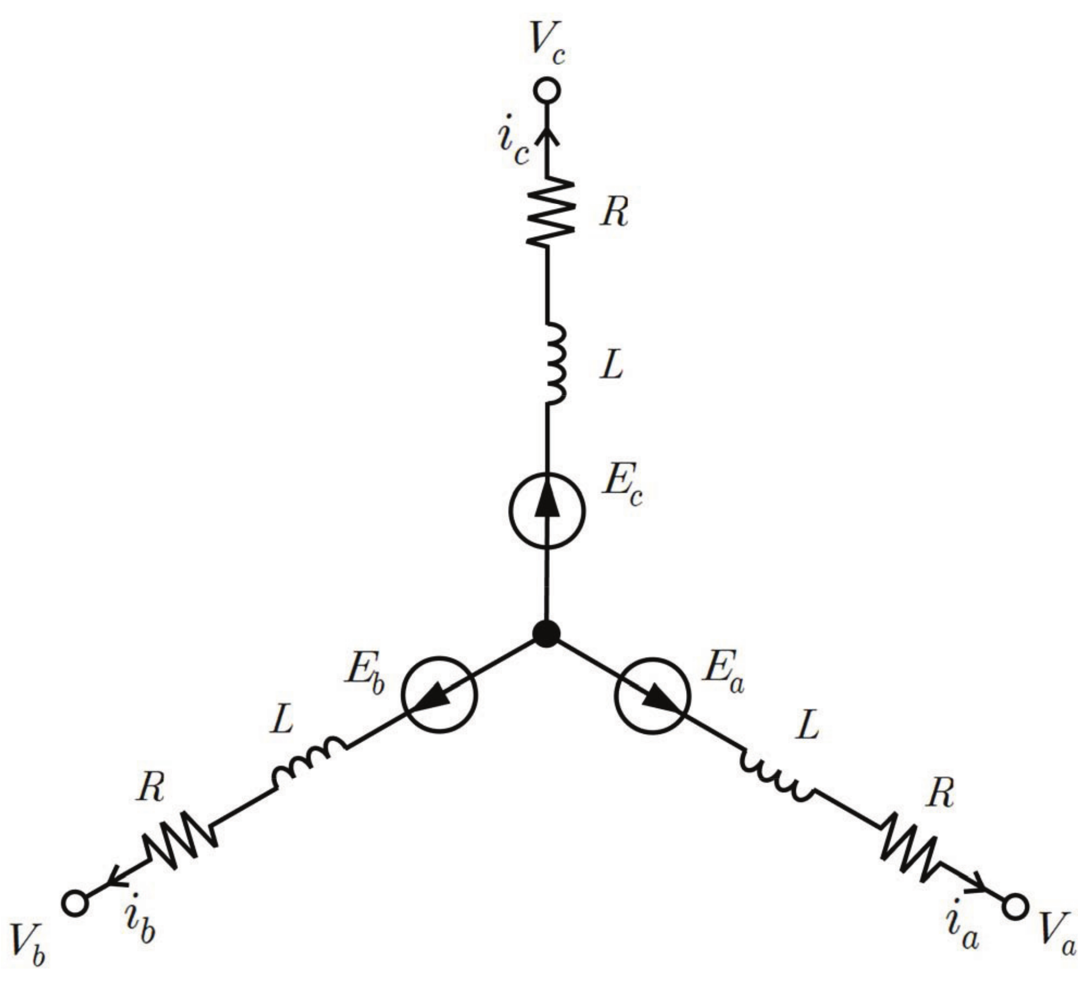
For the electrical part, the three phase equivalent circuit of the BLDCM is shown in Figure 1.

From Figure 1, the voltage equations of the BLDCM can be written as

$$\begin{array}{c}\hfill \begin{array}{cc}\hfill V_a& =R{i}_a+L{\dot{i}}_a+E_a\hfill \\ \hfill V_b& =R{i}_b+L{\dot{i}}_b+E_b\hfill \\ \hfill V_c& =R{i}_c+L{\dot{i}}_c+E_c\hfill \end{array}\end{array}$$

(4)

where $V_a$, $V_b$, and $V_c$ are the input voltages of each phase, respectively. R and L are the phase resistance and phase inductance, respectively. $E_a$, $E_b$, and $E_c$ are the back-EMFs of each phase, respectively. Using (3) and (4), the BLDCM dynamics can be represented as

$$\begin{array}{c}\hfill \begin{array}{cc}\hfill {\dot{\theta }}_m& ={\omega }_m\hfill \\ \hfill {\dot{\omega }}_m& =\frac{1}{J_m}(\tau -F_m{\omega }_m-{\tau }_L)\hfill \\ \hfill {\dot{i}}_a& =\frac{1}{L}[V_a-R{i}_a-E_a]\hfill \\ \hfill {\dot{i}}_b& =\frac{1}{L}[V_b-R{i}_b-E_b]\hfill \\ \hfill {\dot{i}}_c& =\frac{1}{L}[V_c-R{i}_c-E_c]\hfill \end{array}\end{array}$$

(5)

The mathematical modeling of the back-EMF is discussed in the next subsection.

2.2. Back-EMF Modeling

To control the position of the BLDCM, it is necessary to generate torque, which is an input to the mechanical dynamics. The torque can be rewritten with the back-EMF and phase currents as follows:

$$\begin{array}{c}\hfill \begin{array}{c}\hfill \tau =\frac{E_a{i}_a+E_b{i}_b+E_c{i}_c}{{\omega }_m}.\end{array}\end{array}$$

(6)

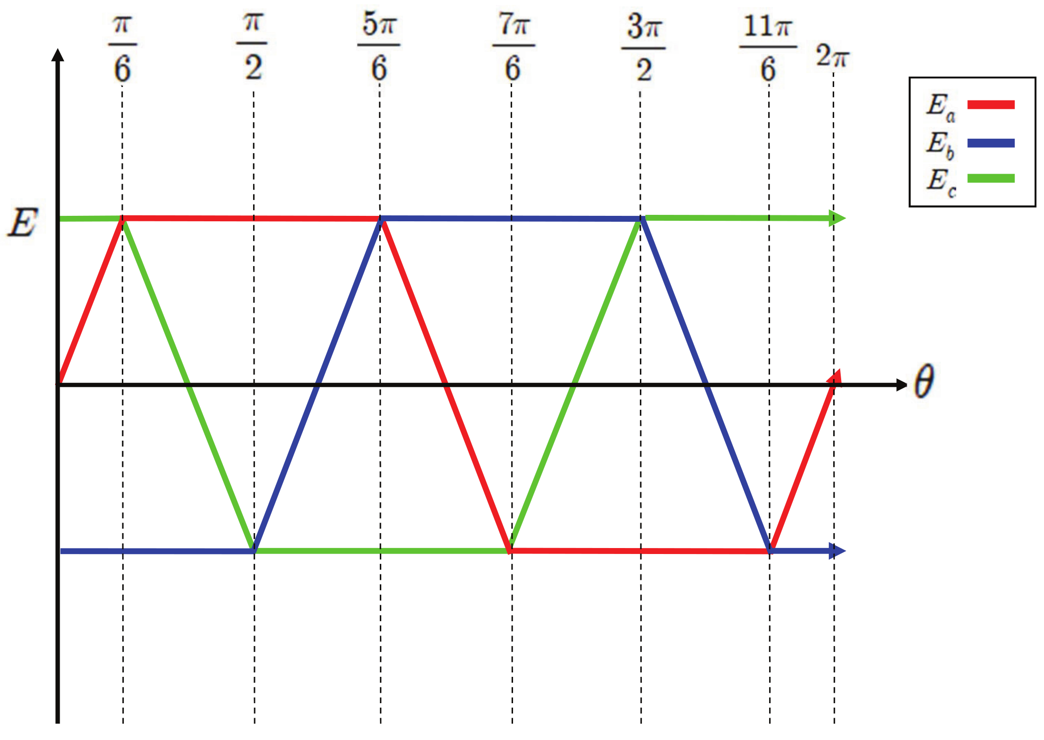
The modeling of the back-EMF is required to generate torque. In a BLDCM, the back-EMF is generally expressed as a trapezoidal nonlinear functions, as shown in Figure 2. The back-EMF functions can be written as

$$\begin{array}{c}\hfill \begin{array}{cc}\hfill E_a& =k_e{\omega }_m{f}_1({\theta }_m)\hfill \\ \hfill E_b& =k_e{\omega }_m{f}_2({\theta }_m)\hfill \\ \hfill E_c& =k_e{\omega }_m{f}_3({\theta }_m)\hfill \end{array}\end{array}$$

(7)

where $k_e$ is back-EMF constant,

$$\begin{array}{c}\hfill \begin{array}{c}\hfill f_1({\theta }_m)=\left\{\begin{array}{cc}\frac{6}{\pi }{\theta }_m& (0\le {\theta }_m<\frac{\pi }{6})\\ 1& (\frac{\pi }{6}\le {\theta }_m<\frac{5\pi }{6})\\ -\frac{6}{\pi }{\theta }_m+6& (\frac{5\pi }{6}\le {\theta }_m<\frac{7\pi }{6})\\ -1& (\frac{7\pi }{6}\le {\theta }_m<\frac{11\pi }{6})\\ \frac{6}{\pi }{\theta }_m+12& (\frac{11\pi }{6}\le {\theta }_m<2\pi )\end{array}\right.\end{array}\end{array}$$

(8)

Similarly, $f_2({\theta }_m)$ and $f_3({\theta }_m)$ can be designed as follows:

$$\begin{array}{c}\hfill \begin{array}{cc}\hfill f_2({\theta }_m)& =f_1({\theta }_m-\frac{2\pi }{3})\hfill \\ \hfill f_3({\theta }_m)& =f_1({\theta }_m+\frac{2\pi }{3}).\hfill \end{array}\end{array}$$

(9)

2.3. Error Dynamics

In this subsection, error dynamics are induced by defining the tracking errors to design the position and current tracking controller based on the model parameters. Let us define the tracking errors of the mechanical and electrical states as below:

$$\begin{array}{c}\hfill \begin{array}{cc}\hfill e_{\theta }& ={\theta }_m^d-{\theta }_m\hfill \\ \hfill e_{\omega }& ={\omega }_m^d-{\omega }_m\hfill \\ \hfill e_a& =i_a^d-i_a\hfill \\ \hfill e_b& =i_b^d-i_b\hfill \\ \hfill e_c& =i_c^d-i_c\hfill \end{array}\end{array}$$

(10)

where ${\theta }_m^d$ and ${\omega }_m^d$ are the desired angular position and desired angular velocity, respectively. $i_a^d$, $i_b^d$, and $i_c^d$ are the desired phase currents of each phase, respectively. Tracking error dynamics can be derived from (10) with respect to time is given by

$$\begin{array}{c}\hfill \begin{array}{cc}\hfill {\dot{e}}_{\theta }& =e_{\omega }\hfill \\ \hfill {\dot{e}}_{\omega }& ={\dot{\omega }}_m^d-{\dot{\omega }}_m\hfill \\ \hfill & =-\frac{1}{J_m}[\tau -J_m{\dot{\omega }}_m^d-F_m{\omega }_m-{\tau }_L]\hfill \\ \hfill {\dot{e}}_a& ={\dot{i}}_a^d-{\dot{i}}_a\hfill \\ \hfill & =\frac{1}{L}[L{\dot{i}}_a^d+R{i}_a+k_e{\omega }_m{f}_1({\theta }_m)-V_a]\hfill \\ \hfill {\dot{e}}_b& ={\dot{i}}_b^d-{\dot{i}}_b\hfill \\ \hfill & =\frac{1}{L}[L{\dot{i}}_b^d+R{i}_b+k_e{\omega }_m{f}_2({\theta }_m)-V_b]\hfill \\ \hfill {\dot{e}}_c& ={\dot{i}}_c^d-{\dot{i}}_c\hfill \\ \hfill & =\frac{1}{L}[L{\dot{i}}_c^d+R{i}_c+k_e{\omega }_m{f}_3({\theta }_m)-V_c]\hfill \end{array}\end{array}$$

(11)

3. Controller Design

This section describes the design of the controller, which consists of two elements: the nonlinear position controller and the current controller.

3.1. Nonlinear Position Controller via Backstepping Approach

In order to improve the tracking performance of the BLDCM for the mechanical part, we designed the torque and mechanical input based on the tracking error dynamics derived in Section 2. First, by substituting (7) into (6) $\tau$ can be rewritten as follows:

$$\begin{array}{c}\hfill \begin{array}{c}\hfill \tau =k_e{f}_1({\theta }_m)i_a+k_e{f}_2({\theta }_m)i_b+k_e{f}_3({\theta }_m)i_c\end{array}\end{array}$$

(12)

therefore, the desired torque can also be defined as

$$\begin{array}{c}\hfill \begin{array}{c}\hfill {\tau }^d=k_e{f}_1({\theta }_m)i_a^d+k_e{f}_2({\theta }_m)i_b^d+k_e{f}_3({\theta }_m)i_c^d\end{array}\end{array}$$

(13)

Using (11) and (12), the mechanical error dynamics can be represented as

$$\begin{array}{c}\hfill \begin{array}{cc}\hfill {\dot{e}}_{\theta }=& e_{\omega }\hfill \\ \hfill {\dot{e}}_{\omega }=& -\frac{1}{J_m}[-J_m{\dot{\omega }}^d-F_m{\omega }_m-{\tau }_L\hfill \\ \hfill & +k_e{f}_1({\theta }_m)(i_a^d-e_a)+k_e{f}_2({\theta }_m)(i_b^d-e_b)+k_e{f}_3({\theta }_m)(i_c^d-e_c)]\hfill \\ \hfill =& -\frac{1}{J_m}[{\tau }^d-J_m{\dot{\omega }}^d-F_m{\omega }_m-{\tau }_L\hfill \\ \hfill & -k_e{f}_1({\theta }_m)e_a-k_e{f}_2({\theta }_m)e_b-k_e{f}_3({\theta }_m)e_c].\hfill \end{array}\end{array}$$

(14)

Theorem 1.

Consider the mechanical error dynamics in (14). If nonlinear position controller is designed as

$$\begin{array}{c}\hfill \begin{array}{c}\hfill {\tau }^d=J_m{\dot{\omega }}^d+F_m{\omega }_m^d+k_1{e}_{\theta }+k_2{e}_{\omega }+{\tau }_{emf}+{\widehat{\tau }}_L\end{array}\end{array}$$

(15)

where${\tau }_{emf}=k_e{f}_1({\theta }_m)e_a+k_e{f}_2({\theta }_m)e_b+k_e{f}_3({\theta }_m)e_c$, $k_1$and$k_2$are the controller gains such that$A_m=\left[\begin{array}{cc}0& 1\\ -\frac{k_1}{J_m}& -\frac{k_2+F_m}{J_m}\end{array}\right]$is Hurwitz,${\widehat{\tau }}_L$is the estimated load torque and is described in next section. Then,$e_{\theta }$and$e_{\omega }$are uniformly ultimately bounded.

Proof. 

With the nonlinear position controller (15), the mechanical error dynamics (14) become

$$\begin{array}{c}\hfill \underset{{\dot{e}}_m}{\underbrace{\left[\begin{array}{c}{\dot{e}}_{\theta }\\ {\dot{e}}_{\omega }\end{array}\right]}}=\underset{A_m}{\underbrace{\left[\begin{array}{cc}0& 1\\ -\frac{k_1}{J_m}& -\frac{k_2+F_m}{J_m}\end{array}\right]}}\underset{e_m}{\underbrace{\left[\begin{array}{c}{e}_{\theta }\\ e_{\omega }\end{array}\right]}}+\underset{B_m}{\underbrace{\left[\begin{array}{c}0\\ \frac{1}{J_m}\end{array}\right]}}{\tilde{\tau }}_L\end{array}$$

(16)

where ${\tilde{\tau }}_L={\tau }_L-{\widehat{\tau }}_L$. For stability analysis, the Lyapunov candidate function, $V_m$, is defined as

$$\begin{array}{c}\hfill \begin{array}{c}\hfill V_m=e_m^T{P}_m{e}_m.\end{array}\end{array}$$

(17)

Because $A_m$ is Hurwitz, the positive matrix $P_m$ exits such that $A_m^T{P}_m+P_m{A}_m=-I$. Then, the derivative of $V_m$ with respect to time is

$$\begin{array}{c}\hfill \begin{array}{cc}\hfill {\dot{V}}_m& =e_m^T(A_m^T{P}_m+P_m{A}_m)e_m+2e_m^T{P}_m{B}_m{\tilde{\tau }}_L\hfill \\ \hfill & \le -\parallel e_m{\parallel }_2+2\parallel e_m\parallel \parallel P_m\parallel B_m{\tilde{\tau }}_L.\hfill \end{array}\end{array}$$

(18)

For $\parallel e_m\parallel \ge 2\parallel P_m\parallel B_m{\tilde{\tau }}_L$,

$$\begin{array}{c}\hfill {\dot{V}}_m\le -{\parallel e_m\parallel }_2.\end{array}$$

(19)

Therefore, it is concluded that $e_m$ is uniformly ultimately bounded [22]. □

3.2. Current Controller

The nonlinear position controller in (15) has been proposed with the assumption that the desired torque ${\tau }^d$ is the input in the mechanical dynamics, and the electrical dynamics is neglected. Since the actual input is not the phase currents but the phase voltages in BLDCM, the torque $\tau$ actually generated by the current is not the desired torque ${\tau }^d$; therefore, the current controller is required to track the desired phase currents $i_a^d$, $i_b^d$, and $i_c^d$. It is evident from (13), that the desired phase currents are determined to generate the desired torque ${\tau }^d$ using the commutation scheme as follows:

$$\begin{array}{c}\hfill \begin{array}{cc}\hfill i_a^d& =\frac{1}{k_e{f}_1({\theta }_m)}\frac{{\tau }^d}{3}\hfill \\ \hfill i_b^d& =\frac{1}{k_e{f}_2({\theta }_m)}\frac{{\tau }^d}{3}\hfill \\ \hfill i_c^d& =\frac{1}{k_e{f}_3({\theta }_m)}\frac{{\tau }^d}{3}.\hfill \end{array}\end{array}$$

(20)

Remark 1.

Torque ripples have been presented around zero crossings of the trapezoidal nonlinear functions (= $f_1({\theta }_m)$, $f_2({\theta }_m)$, and $f_3({\theta }_m)$) in Figure 2 because the singularity problem occurs when the denominator in (20) becomes 0; therefore, the values of the trapezoidal nonlinear functions can be replaced with a small real number ϵ, when the trapezoidal nonlinear functions are zero.

Theorem 2.

Consider the electrical error dynamics in (14). If the current controller is developed to track the error dynamics in (14) as

$$\begin{array}{c}\hfill \begin{array}{cc}\hfill V_a& =L{\dot{i}}_a^d+R{i}_a^d+k_e{\omega }_m{f}_1({\theta }_m)+k_3{e}_a\hfill \\ \hfill V_b& =L{\dot{i}}_b^d+R{i}_b^d+k_e{\omega }_m{f}_2({\theta }_m)+k_4{e}_b\hfill \\ \hfill V_c& =L{\dot{i}}_c^d+R{i}_c^d+k_e{\omega }_m{f}_3({\theta }_m)+k_5{e}_c\hfill \end{array}\end{array}$$

(21)

where$k_3$, $k_4$, and $k_5$are the control gains of the current controller and positive constant, respectively, then the origin of the electrical error dynamics in (14) is exponentially stable.

Proof. 

The Lyapunov candidate function, $V_e$ is defined as

$$\begin{array}{c}\hfill \begin{array}{c}\hfill V_e=\frac{1}{2}{e}_a^2+\frac{1}{2}{e}_b^2+\frac{1}{2}{e}_c^2\end{array}\end{array}$$

(22)

Differentiating $V_e$ with respect to time yields

$$\begin{array}{c}\hfill \begin{array}{cc}\hfill {\dot{V}}_e=& e_a{\dot{e}}_a+e_b{\dot{e}}_b+e_c{\dot{e}}_c\hfill \\ \hfill =& \frac{1}{L}[L{\dot{i}}_a^d+R{i}_a+k_e{\omega }_m{f}_1({\theta }_m)-V_a]e_a+\frac{1}{L}[L{\dot{i}}_b^d+R{i}_b+k_e{\omega }_m{f}_2({\theta }_m)-V_b]e_b\hfill \\ \hfill & +\frac{1}{L}[L{\dot{i}}_c^d+R{i}_c+k_e{\omega }_m{f}_3({\theta }_m)-V_c]e_c\hfill \end{array}\end{array}$$

(23)

Substituting the control law from (21) in (22) results in

$$\begin{array}{c}\hfill \begin{array}{cc}\hfill {\dot{V}}_e=& -\frac{R+k_3}{L}{e}_a^2-\frac{R+k_4}{L}{e}_b^2-\frac{R+k_5}{L}{e}_c^2\hfill \end{array}\end{array}$$

(24)

From Equation (24), the conditions obtained are

$$\begin{array}{c}\hfill \begin{array}{c}\hfill k_3>-R,k_4>-R,k_5>-R.\end{array}\end{array}$$

(25)

Because R is a positive constant parameter and the control gains should have positive constant, the origin of the electrical error dynamics in (14) is exponentially stable. □

Using (15), (20), and (21), the proposed method can be summarized as follows:

$$\begin{array}{c}\hfill \begin{array}{cc}\hfill {\tau }^d& =J_m{\dot{\omega }}^d+F_m{\omega }_m^d+k_1{e}_{\theta }+k_2{e}_{\omega }+{\tau }_{emf}\hfill \\ \hfill i_a^d& =\frac{1}{k_e{f}_1({\theta }_m)}\frac{{\tau }^d}{3}\hfill \\ \hfill i_b^d& =\frac{1}{k_e{f}_2({\theta }_m)}\frac{{\tau }^d}{3}\hfill \\ \hfill i_c^d& =\frac{1}{k_e{f}_3({\theta }_m)}\frac{{\tau }^d}{3}\hfill \\ \hfill V_a& =L{\dot{i}}_a^d+R{i}_a^d+k_e{\omega }_m{f}_1({\theta }_m)+k_3{e}_a\hfill \\ \hfill V_b& =L{\dot{i}}_b^d+R{i}_b^d+k_e{\omega }_m{f}_2({\theta }_m)+k_4{e}_b\hfill \\ \hfill V_c& =L{\dot{i}}_c^d+R{i}_c^d+k_e{\omega }_m{f}_3({\theta }_m)+k_5{e}_c.\hfill \end{array}\end{array}$$

(26)

4. Augmented Observer Design and Closed-Loop Stability

In the previous section, the controller was designed using the known state variables. To develop a nonlinear position controller, it is necessary to determine the load torque (disturbance). This section describes the design of an augmented observer to compensate for the load torque as a disturbance. Subsequently, the closed-loop stability is discussed.

4.1. Augmented Observer Design

In practice, the load torque varies considerably slowly; therefore, it can be reasonably assumed that ${\dot{\tau }}_L=0$. Referring to the BLDCM modeling in (3) and allowing the augmented state vector $x_a={\left[\begin{array}{ccc}{\tau }_L& {\theta }_m& {\omega }_m\end{array}\right]}^T$, the augmented system of the mechanical system in (3) can be represented as follows:

$$\begin{array}{c}\hfill \begin{array}{cc}\hfill {\dot{\tau }}_L& =0\hfill \\ \hfill {\dot{\theta }}_m& ={\omega }_m\hfill \\ \hfill {\dot{\omega }}_m& =\frac{1}{J_m}(\tau -F_m{\omega }_m-{\tau }_L)\hfill \end{array}\end{array}$$

(27)

Based on (27), we proposed the augmented observer to estimate the mechanical states and disturbance (load torque) as follows:

$$\begin{array}{c}\hfill \begin{array}{cc}\hfill {\dot{\widehat{\tau }}}_L& =l_1({\theta }_m-{\widehat{\theta }}_m)\hfill \\ \hfill {\dot{\widehat{\theta }}}_m& ={\widehat{\omega }}_m+l_2({\theta }_m-{\widehat{\theta }}_m)\hfill \\ \hfill {\dot{\widehat{\omega }}}_m& =\frac{1}{J_m}(\tau -F_m{\widehat{\omega }}_m-{\widehat{\tau }}_L)+l_3({\theta }_m-{\widehat{\theta }}_m)\hfill \end{array}\end{array}$$

(28)

where ${\tau }_L$, $\widehat{\theta }$, and $\widehat{\omega }$ are estimated disturbance, estimated angular position, and estimated angular velocity, respectively. Thus, the estimation errors are defined as

$$\begin{array}{c}\hfill \begin{array}{cc}\hfill {\tilde{\tau }}_L& ={\tau }_L-{\widehat{\tau }}_L\hfill \\ \hfill {\tilde{\theta }}_m& ={\theta }_m-{\widehat{\theta }}_m\hfill \\ \hfill {\tilde{\omega }}_m& ={\omega }_m-{\widehat{\omega }}_m\hfill \end{array}\end{array}$$

(29)

By differentiating the augmented states ${\tau }_L$, $\widehat{\theta }$, and $\widehat{\omega }$ with respect to time, the estimation error dynamics can be derived as

$$\begin{array}{c}\hfill \begin{array}{c}\hfill {\dot{\tilde{x}}}_a=A_o{\tilde{x}}_a\end{array}\end{array}$$

(30)

where ${\tilde{x}}_a=\left[\begin{array}{ccc}{\tilde{\tau }}_L& {\tilde{\theta }}_m& {\tilde{\omega }}_m\end{array}\right]$, $A_o=\left[\begin{array}{ccc}0& -l_1& 0\\ 0& -l_2& 1\\ -\frac{1}{J_m}& -l_3& -\frac{F_m}{J_m}\end{array}\right]$.

Theorem 3.

Given the augmented observer in (28), if $l_1$ is negative, $l_2$ and $l_3$ are positive, the condition $P_3>0$ is satisfied. Then, the estimation errors exponentially converge to zero.

Proof. 

For a given matrix $A_o$, we have the closed-loop characteristic equation as

$$\begin{array}{c}\hfill \begin{array}{c}\hfill {\lambda }^3+\left(\frac{F_m+J_m{l}_2}{J_m}\right){\lambda }^2+\left(\frac{F_m{l}_2+l_3}{J_m}\right)\lambda -\frac{l_1}{J_m}=0\end{array}\end{array}$$

(31)

where $\lambda$ is the characteristic roots of $A_o$. We can use the Routh–Hurwitz criterion to determine the characteristic roots of (31); therefore, the Routh–Hurwitz table is as follows:

(32)

A closed-loop system is stable if there are no sign changes in the first column of the Routh–Hurwitz table; therefore, the estimation errors exponentially converge to zero if $l_1$ is negative and $l_2$, $l_3$, and $P_3$ are positive. □

4.2. Closed-Loop Stability

As described in the previous sections, the nonlinear position controller, current controller, and augmented observer were independently designed. Thus, the stability of a closed-loop system should be considered. The closed-loop system is defined as follows:

$$\begin{array}{c}\hfill \begin{array}{cc}\hfill \dot{e}& =A_{e}e+B_e{\tilde{x}}_a\hfill \\ \hfill {\dot{\tilde{x}}}_a& =A_o{\tilde{x}}_a\hfill \end{array}\end{array}$$

(33)

where

$$\begin{array}{c}\hfill A_e=\left[\begin{array}{ccccc}0& 1& 0& 0& 0\\ -\frac{k_1}{J_m}& -\frac{k_2+F_m}{J_m}& 0& 0& 0\\ 0& 0& -\frac{k_3+R}{L}& 0& 0\\ 0& 0& 0& -\frac{k_4+R}{L}& 0\\ 0& 0& 0& 0& -\frac{k_5+R}{L}\end{array}\right],B_e=\left[\begin{array}{ccc}0& 0& 0\\ \frac{1}{J_m}& 0& 0\\ 0& 0& 0\\ 0& 0& 0\\ 0& 0& 0\end{array}\right].\end{array}$$

(34)

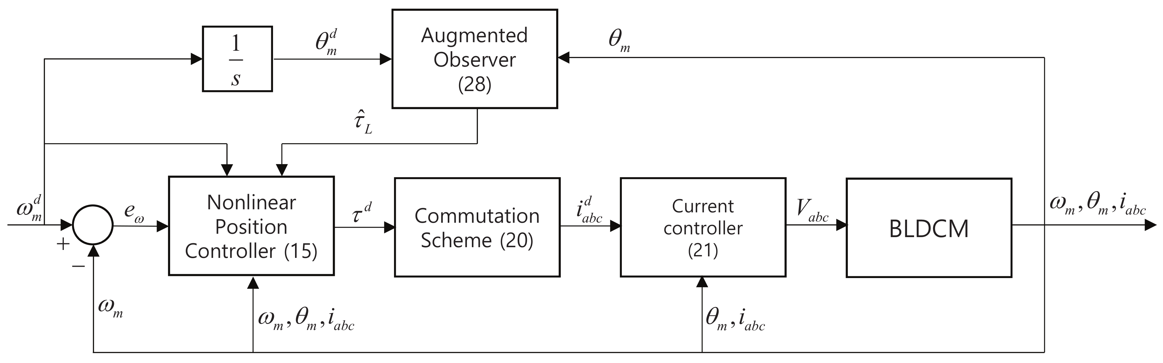
In the closed-loop system in (33), $A_e$ and $A_o$ are Hurwitz and $B_e$ is bounded. Thus, $e_{\theta }$, $e_{\omega }$, $e_a$, $e_b$, and $e_c$ are input-to-state stable because it was proven that ${\tilde{x}}_a$ exponentially converge to zero in the previous subsection [22]. Control block diagram of the proposed method is shown in Figure 3.

5. Simulation Results

Simulations were performed to evaluate the performance of the proposed controller. The BLDCM parameters and control gains of the nonlinear position controller and current controller, in addition to the augmented observer gains used in the simulation, are listed in

Table 1. BLDCM Plant parameters and control gains.

BLDCM Plant Parameters and Control Gains
BLDCM Plant parameters	$F_m$	$0.10625\times {10}^{-3}$ [Nm/rad/s]
	$J_m$	$8.5\times {10}^{-6}$ [Kg·m2]
	L	55 [Ω]
	R	0.215 [mH]
	$k_e$	2 [V/rad/s]
Nonlinear position controller gains	$k_1$	0.25
	$k_2$	2
Current controller gains	$k_3$	80
	$k_4$	80
	$k_5$	80
Conventional PI controller gains (outer-loop)	$k_P$	0.5
	$k_I$	8
Conventional PI controller gains (inner-loop)	$k_P$	1
	$k_I$	$1\times {10}^6$
Augmented observer gains	$l_1$	$-1\times {10}^3$
	$l_2$	$2\times {10}^3$
	$l_3$	$5\times {10}^6$

. We performed simulations using the following two cases:

• Case 1: conventional PI controller.
• Case 2: proposed controller.

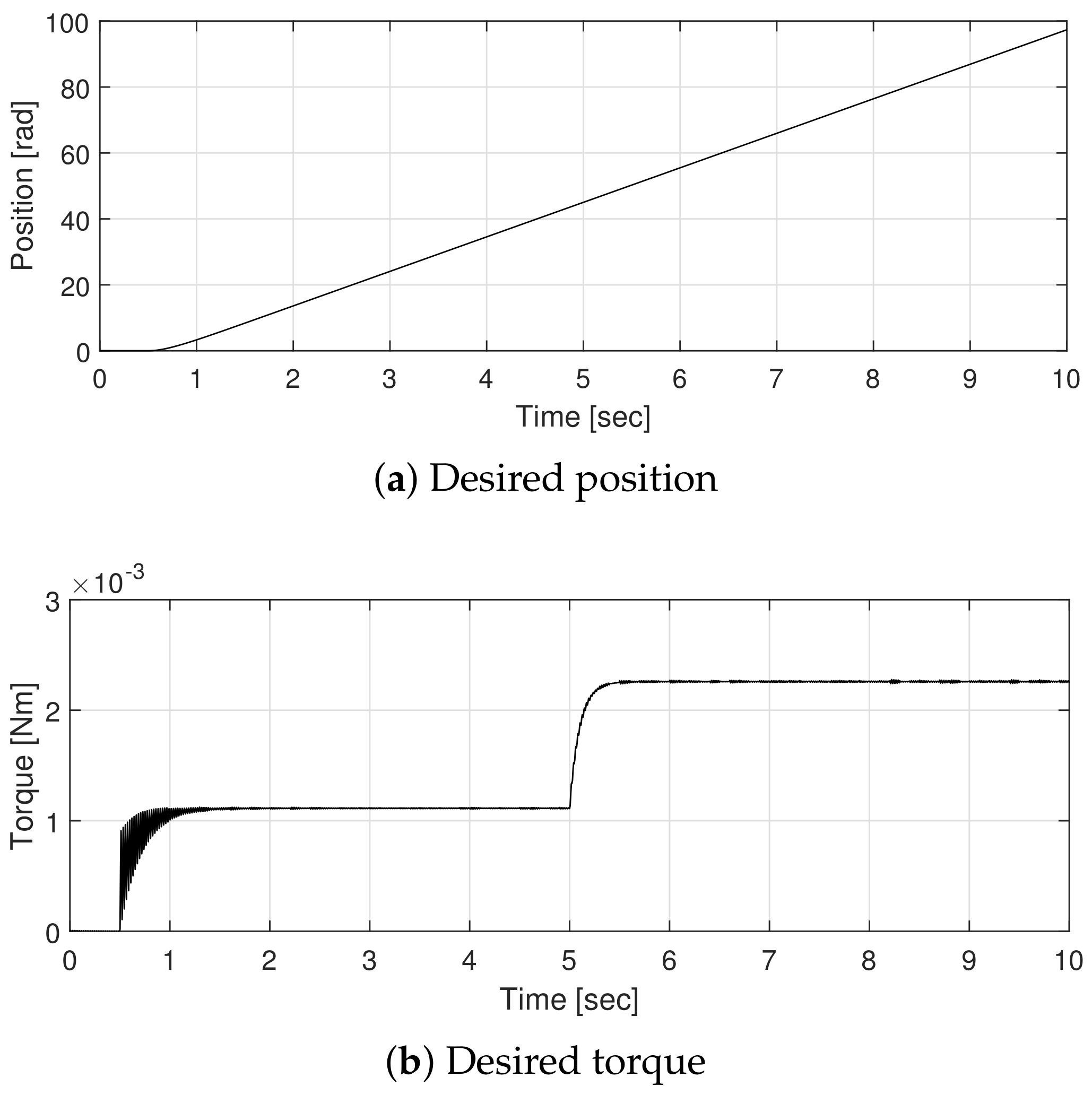
To confirm the estimation performance, the step load torque was injected at 5 s. The desired angular velocity and the desired torque are shown in Figure 4. In the steady-state region, the desired angular velocity was set to 100 rpm. The desired torque was generated to compensate for the load torque by implementing (15) from the nonlinear position controller.

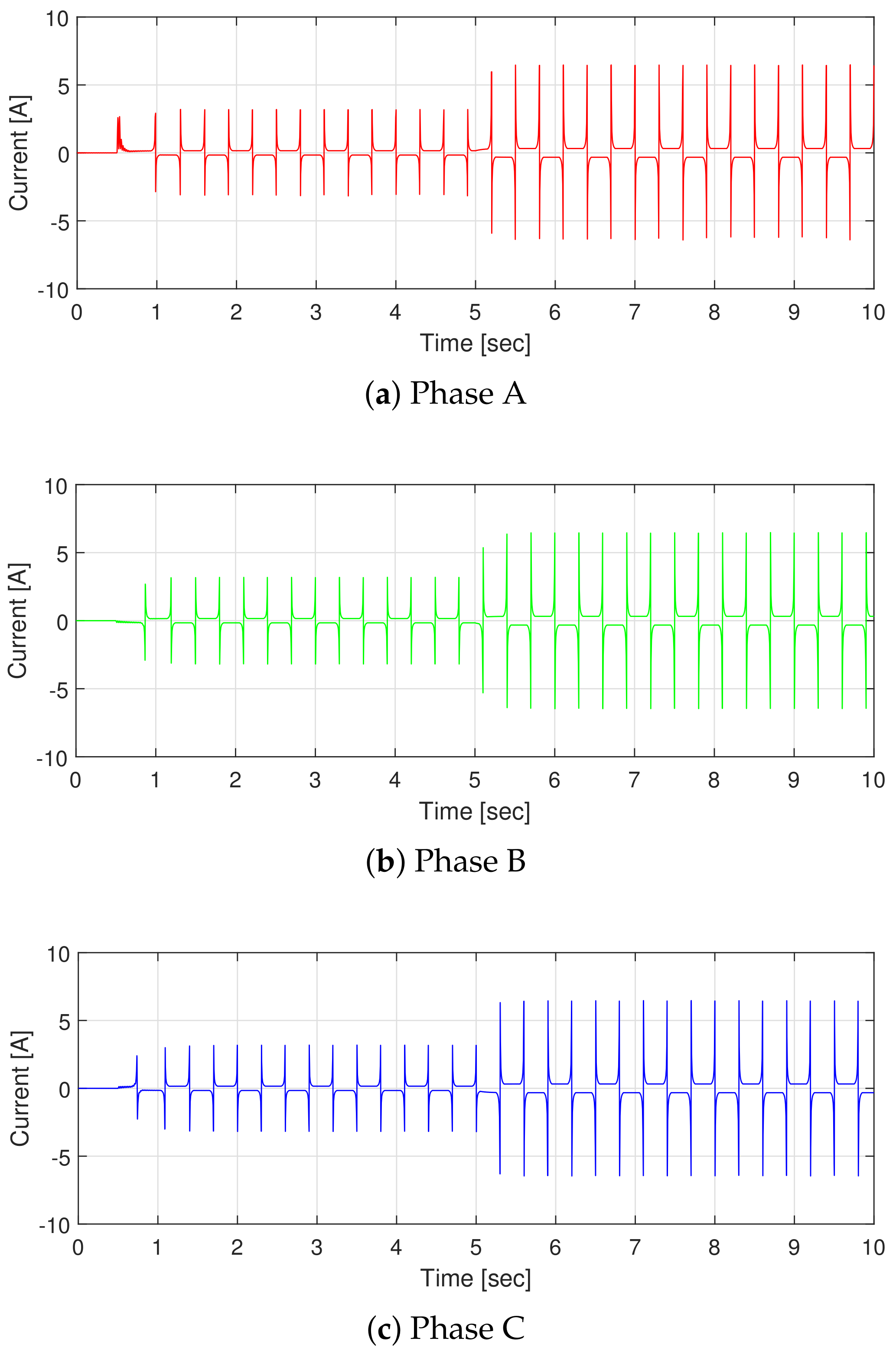
Figure 5 shows the desired phase currents, which were calculated using (20). The ripples observed in the desired phase currents were the largest when back-EMFs became zero. The ripple frequency was approximately 3.33 Hz, which is the 2nd harmonics of the fundamental desired velocity (100 rpm ≈ 1.66 Hz). In particular, it can be observed that the amplitude of the desired phase currents increased after 5 s because the desired torque increased owing to the injected load torque.

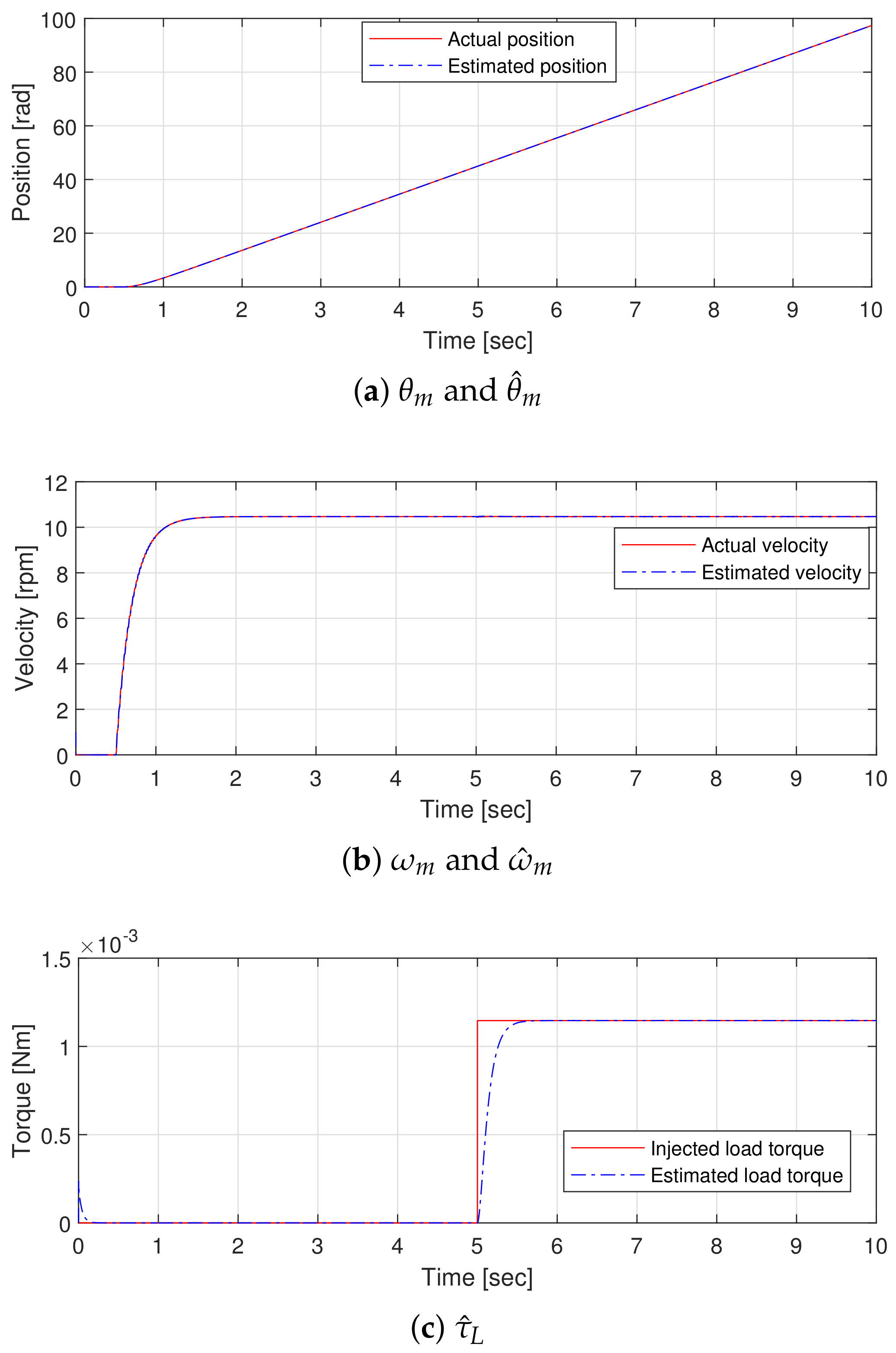
Figure 6 shows estimation performance of the proposed augmented observer. The estimated angular position and estimated angular velocity sufficiently tracked the actual position and actual velocity, respectively, using the proposed augmented observer. Thus, the load torque was well estimated and the estimated load torque was added to control input to generate the desired torque for the load torque rejection.

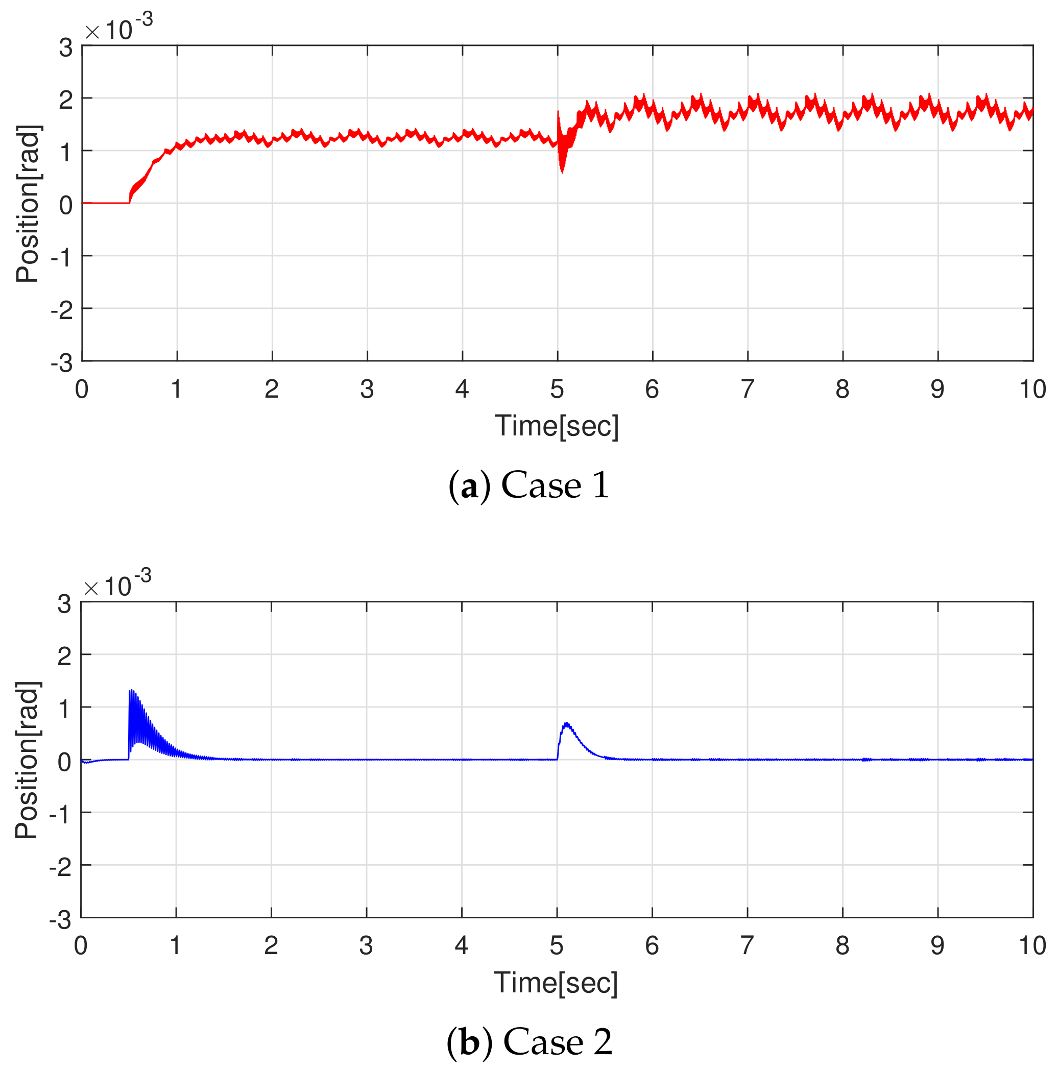
Figure 7 shows position tracking performances under the two cases. In Case 1, the steady-state tracking error was inevitable because conventional PI controller does not guarantee the exponential convergence of the position tracking error. By contrast, the tracking error of the proposed method converged to zero in the steady-state region. After the load torque was injected, it is evident that the position tracking error converged to 0 within 1 s in the proposed method, whereas the position tracking error became higher than before in the conventional PI control method. In Case 2, the robust position tracking performance could be guaranteed because the load torque estimated using the proposed augmented observer was considered as the control input.

6. Conclusions

In this study, a position control method was developed to reduce the tracking errors caused by torque ripples. The proposed method comprises a nonlinear position controller, a current controller, and an augmented observer. The nonlinear position controller was designed to generate the desired torque based on the error dynamics. The desired torque generated by the nonlinear position controller was transformed into the desired phase currents. A current controller that tracks the desired phase current was also developed to track the desired torque. Subsequently, the load torque was compensated using the estimated load torque obtained from the augmented observer. In the simulations, we observed that all the state variables and the load torque were well estimated. In addition, the velocity ripple was reduced, as compared to that for the conventional PI controller. In the proposed method, the position tracking error converged to zero nearly while the position tracking error was not effectively reduced by the conventional PI controller. When the load torque was injected, the proposed method had a better dynamic response compared with the conventional PI controller.

References

- Maharajan, M.P.; Xavier, S.A.E. Design of speed control and reduction of torque ripple factor in BLdc motor using spider based controller. IEEE Trans. Power Electron. 2019, 34, 7826–7837. [Google Scholar] [CrossRef]
- Fang, J.; Zhou, X.; Liu, G. Instantaneous torque control of small inductance brushless DC motor. IEEE Trans. Power Electron. 2012, 27, 4952–4964. [Google Scholar] [CrossRef]
- Low, T.-S.; Lee, T.-H.; Tseng, K.-J.; Lock, K.-S. Servo performance of a BLDC drive with instantaneous torque control. IEEE Trans. Ind. Appl. 1992, 28, 455–462. [Google Scholar] [CrossRef]
- Bae, J.; Lee, D.-H. Position control of a rail guided mover using a low-cost BLDC motor. IEEE Trans. Ind. Appl. 2018, 54, 2392–2399. [Google Scholar] [CrossRef]
- Dat, N.T.; Kien, C.V.; Anh, H.P.H. Optimal FOC-PID parameters of BLDC motor system control using parallel PM-PSO optimization technique. Int. J. Comput. Intell. Syst. 2021, 1, 1141–1154. [Google Scholar]
- Ozturk, S.B.; Toliyat, H.A. Direct torque and indirect flux control of brushless DC motor. IEEE/ASME Trans. Mechatron. 2011, 16, 351–360. [Google Scholar] [CrossRef]
- Krishnamurthy, P.; Khorrami, F. An analysis of the effects of closed-loop commutation delay on stepper motor control and application to parameter estimation. IEEE Trans. Control Syst. Technol. 2008, 16, 70–77. [Google Scholar] [CrossRef]
- Wu, Y.; Deng, Z.; Wang, X.; Ling, X.; Cao, X. Position sensorless control based on coordinate transformation for brushless DC motor drives. IEEE Trans. Power Electron. 2010, 25, 2365–2371. [Google Scholar] [CrossRef]
- Hernández-Guzmán, V.M.; Orrante-Sakanassi, J. PID control of robot manipulators actuated by BLDC motors. Int. J. Control 2021, 94, 267–276. [Google Scholar] [CrossRef]
- Immaneni, H. Mathematical modelling and position control of brushless Dc (Bldc) motor. Int. J. Eng. Res. Appl. 2013, 3, 1050–1057. [Google Scholar]
- Stirban, A.; Boldea, I.; Andreescu, G.-D. Motion-sensorless control of BLDC-PM motor with offline FEM-information-assisted position and speed observer. IEEE Trans. Ind. Appl. 2012, 48, 1950–1958. [Google Scholar] [CrossRef]
- Ba, D.X.; Yeom, H.; Kim, J.; Bae, J. Gain-adaptive robust backstepping position control of a BLDC motor system. IEEE/ASME Trans. Mechatron. 2018, 23, 2470–2481. [Google Scholar]
- Ko, J.S.; Youn, S.K.; Bose, B.K. A study on adaptive load torque observer for robust precision position control of BLDC motor. In Proceedings of the IECON’99, Conference Proceedings, 25th Annual Conference of the IEEE Industrial Electronics Society (Cat. No. 99CH37029), San Jose, CA, USA, 29 November–3 December 1999; pp. 1091–1096. [Google Scholar]
- Darba, A.; D’haese, P.; De Belie, F.; Melkebeek, J.A. Improving the dynamic stiffness in a self-sensing BLDC machine drive using estimated load torque feedforward. IEEE Trans. Ind. Appl. 2015, 51, 3101–3114. [Google Scholar] [CrossRef]
- De Wit, C.C.; Olsson, H.; Astrom, K.J.; Lischinsky, P. A new model for control of systems with friction. IEEE Trans. Autom. Control 1995, 40, 419–425. [Google Scholar] [CrossRef] [Green Version]
- Ding, S.; Chen, W.-H.; Mei, K.; Murray-Smith, D.J. Disturbance observer design for nonlinear systems represented by input output models. IEEE Trans. Ind. Electron. 2020, 67, 1222–1232. [Google Scholar] [CrossRef] [Green Version]
- Delibas, B.; Koc, B. A method to realize low velocity movability and eliminate friction induced noise in piezoelectric ultrasonic motors. IEEE/ASME Trans. Mechatron. 2020, 25, 2677–2687. [Google Scholar] [CrossRef]
- Lin, C.; Yau, H.; Tian, Y. Identification and compensation of nonlinear friction characteristics and precision control for a linear motor stage. IEEE/ASME Trans. Mechatron. 2013, 18, 1385–1396. [Google Scholar] [CrossRef]
- Slotine, J.; Weiping, L.W. Applied Nonlinear Control; Prentice-Hall: London, UK, 1991; pp. 331, 365. [Google Scholar]
- Conte, G.; Moog, C.; Perdon, A. Algebraic Methods for Nonlinear Control Systems; Springer: London, UK, 2007. [Google Scholar]
- Young, K.D.; Utkin, V.I.; Ozguner, U. A control engineers guide to sliding mode control. IEEE Trans. Control Syst. Technol. 1999, 7, 328–342. [Google Scholar] [CrossRef] [Green Version]
- Khalil, H. Nonlinear Systems, 3rd ed.; Prentice-Hall: Englewood Cliffs, NJ, USA, 2002. [Google Scholar]
Publisher’s Note: MDPI stays neutral with regard to jurisdictional claims in published maps and institutional affiliations. |
© 2021 by the authors. Licensee MDPI, Basel, Switzerland. This article is an open access article distributed under the terms and conditions of the Creative Commons Attribution (CC BY) license (https://creativecommons.org/licenses/by/4.0/).