Abstract
One of the most favorable renewable energy sources, solar photovoltaic (PV) can meet the electricity demand considerably. Sunlight is converted into electricity by the solar PV systems using cells containing semiconductor materials. A PV system is designed to meet the energy needs of King Abdulaziz University Hospital. A new method has been introduced to find optimal working capacity, and determine the self-consumption and sufficiency rates of the PV system. Response surface methodology (RSM) is used for determining the optimal working conditions of PV panels. Similarly, an adaptive neural network based fuzzy inference system (ANFIS) was employed to analyze the performance of solar PV panels. The outcomes of methods were compared to the actual outcomes available for testing the performance of models. Hence, for a 40 MW target PV system capacity, the RSM determined that approximately 33.96 MW electricity can be produced, when the radiation rate is 896.3 W/m2, the module surface temperature is 41.4 °C, the outdoor temperature is 36.2 °C, the wind direction and speed are 305.6 and 6.7 m/s, respectively. The ANFIS model (with nine rules) gave the highest performance with lowest residual for the same design parameters. Hence, it was determined that the hourly electrical energy requirement of the hospital can be met by the PV system during the year.
Keywords:
solar PV module; performance prediction; simulation; self-consumption model; RSM; ANFIS; hospital 1. Introduction
The energy planning systems have transformed from specific objectives with constraints to more complex approaches due to the insertion of multiple criteria, investors and needs of nations that are usually in conflict. Renewable and non-renewable energy sources are the basis of different energy systems. The world energy need is presently met mainly from fossil fuels (81%), renewable energy (14%), and nuclear sources (5%) [1]. Fossil fuels are disposable, and unsafe for the environment due to their impacts on climate and pollution rising. Similarly, nuclear sources and power reactors are deemed dangerous by some scientists as a result of their high capital costs, the power systems’ control, opposing public opinion, nuclear waste management, and economies of the scale envisaged. However, they have many advantages such as lower emissions, higher security of supply and enabling of possible other technologies. The major direction of the world is to develop independent small nuclear units for energy generation that bring greater simplicity of design, short construction times, and reduced siting costs. On the other hand, small nuclear units are much more easily manageable investments whose costs often rival the capitalization of large plants. Renewable energy sources alleviate their downsides, and eventually cost less than fossil fuels that own useless production technologies. For instance, due to urgent environmental pollution and climate change issues, using a mix of fossil fuels and renewable energy sources, Italy carried out an ‘energy transition’ towards a more sustainable energy production and consumption system by adopting nuclear power to reduce the consumption of fossil fuels [2]. Solar photovoltaic (PV) as a favorable renewable energy source can meet the electricity demand of Saudi Arabia providing a 50 GW additional capacity. However, the aggregate global renewable energy capacity has reached 227 GW in recent times [3]. The average sunlight energy falling on Kingdom’s land is about 2200 thermal kWh/m2 per year which is acceptably higher when compared to some countries heavily investing in solar energy generation technologies. During the summer seasons, the electricity need reaches its peak load, which is twice higher than in the winter. Therefore, it is worthwhile to generate clean solar PV energy via sunlight [4]. In Saudi Arabia, the electricity consumption is estimated to exceed 40 GW nowadays and reach 120 GW per hour until the year 2028. The electricity consumption of industrial and service sectors is increasing about 6.9% per year mainly due to the investments and capacity expansions. This growth will require more fossil fuel consumption and eventually release a higher amount of CO2 into the atmosphere. Although the Kingdom’s annual solar irradiance is about 2000–2450 kWh/m2, the availability of immense empty lands and ideal locations for solar installations and PV generation [4]; the renewable energy share of Kingdom is still less than 0.1%, compared to 14% share of the rest of the world [5]. In this context, Alnaser and Alnaser [6] claimed that only 0.1% of Kingdom’s land is sufficient for the solar PV projects to meet the electricity demand estimated for 2050. Many countries are interested in reliable, sustainable, suitable, and diversified energy sources, and technologies due to the pros and cons of non-renewable energy sources and technologies. The challenging problem for a country is the determination of the proper energy sources and technologies for the public and private investments. Although Saudi Arabia has wind, and geothermal resources that can solve all energy demand in the future, the new PV technologies are more productive and can generate more energy efficiently. This study also aims to encourage government bodies and private organizations to invest in solar PV energy generation systems for achieving sustainable energy infrastructure.
A solar photovoltaic (PV) system aims to convert sunlight directly into electricity using PV cells. This system uses solar modules consisting of various solar cells containing semiconductor materials. Yildirim and Aktacir [7] investigated the efficiency of PV cells, the parameters affecting photovoltaic panel performance, and variabilities depending on PV technologies. Martin et al. [8] reported that the efficiency of converting solar energy into electrical energy is 9% using organic modules, which can reach 25% using crystalline modules. Monocrystalline, Multi-crystalline and thin film Silicone are broadly used in those PV technologies available which have the highest market share [7]. The most efficient PV modules are obtained from Monocrystalline technology, even highly more efficient than multi-crystalline technology are considered the leader of PV technologies [9] in industry. On the other hand, although solar radiation has the greatest influence on the power of the PV module [10] obtained, the module surface temperature affected by the wind speed and outdoor temperature are also important parameters. The wind speed and its direction have a cooling effect on the temperature of the PV module surface and significantly increase the electricity generation [11,12]. Kalledis et al. [10] have reported that the PV module surface temperature is reduced with rising wind speed. Although certain values of different parameters are considered as the ideal conditions, the reality is usually different, and the parameters do not represent the optimal field circumstances in which the PV panel operates [13].
Today, many studies in the literature related to renewable energy sources consider them as the alternative to fossil energy sources. Taylan et al. [1] used multi-criteria group decision making approaches for determining the attributes of energy sources, and selected technologies for PV energy generation. Lee [14] investigated the energy systems’ essentials for the global economy to produce friendly new technologies for investment. Fan [15] stated that using energy more effectively results in energy efficient systems and reduces direct operating costs and initial investment costs. Tian et al. [16] built an energy evaluation procedure to integrate uncertain factors using stochastic models. Taylan et al. [1] used the experts’ opinions and machine learning approaches to find out that solar PV was an attractive energy system for investment in the Kingdom. The regular daylight in the Kingdom is 12 h 8 min and 48 s on average, longer than several countries using solar PV systems extensively for energy generation. Akpolat et al. [17] investigated a PV system installed for a faculty building and found out that an 84.75-kWp grid- system can produce remarkable power and save about 90.298 kWh of energy annually for faculty buildings. Muteri et al. [18] summarized the current literature of life cycle assessment applied to different types of grid-connected PV systems to critically analyze the results related to energy and environmental impacts generated during the life cycle of PV technologies to provide information for future analyses. Yet, PV modules have 0.09 US$/kWh, however, diesel generators on average have 0.25 US$/kWh levelized electricity cost. Pradhan et al. [19] carried out a comparative analysis about different possible PV configurations in detail and found that the hybrid solar PV-wind energy system is the most suitable energy generation system. Almarshoud [20] examined the performance of a pilot PV system based on real time solar radiation data in 32 sites. Mittal et al. [21] used artificial neural networks (ANNs) to predict the PV Modules performance. Yahya-Khotbehsara, and Shahhoseini [22] merged the numerical and analytical approaches to determine the PV module parameters of Monocrystalline, Multi-crystalline and thin film technologies. Goverde et al. [23] investigated the PV module surface spatial temperature differences affected by wind. Goossens et al. [24] used wind tunnel experiments to investigate the influence of wind flow, and temperature patterns on the electrical performance of buildings integrated with PV modules. Curto et al. [25] investigated the economic impacts of feasibly generating energy from solar, wind and sea wave plants to achieve specific targets of decarbonization in Lampedusa, a small Italian island where currently the energy is supplied totally by diesel power plants. Awan et al. [26] determined that the northern province, Tabuk, is the most feasible region for a solar PV plant. Rani et al. [27] proposed a fuzzy TOPSIS approach for ranking the status of renewable energy sources. Daus et al. [28] calculated the unit cost of generated electric energy from solar PV for the utility sector, health facilities, housing, industrial enterprises, recreation areas and agricultural industries. Yoomak et al. [29] searched the location problem and its effect on the performance assessment of solar PV systems installed on the rooftop of residences in distinct regions of Thailand. Kassem et al. [30] analyzed the solar radiation of five distinct locations in Northern Cyprus statistically in addition to some meteorological parameters such as relative humidity, air temperature, sunshine, and solar radiation. Ascencio-Vásquez et al. [31] used the performance of PV systems to evaluate the risks occurring due to the diverse climate conditions for standardizing the evaluation criteria in regions. Zell et al. [32] believed that understanding the spatial and temporal variability requires considerably more data to optimize the planning and setting of solar energy power plants. Roy et al. [33] studied the features of perovskite solar cells and found them superior to the existing PV technologies for presenting the efficiency and various architectures used to date. Naderloo (2020) [34] predicted the solar radiation using ANN methods, ANFIS and RSM, carried out the sensitivity analysis, and found out that ANNs and RSM were superior to the ANFIS. Benmouiza and Cheknane (2019) [35] used fuzzy c-means (FCM), subtractive clustering, and grid partitioning algorithms to develop an ANFIS for forecasting solar radiation. The findings depicted that the ANFIS model developed with the FCM clustering algorithm gave the best results considering the RMSE approach of 112 W/m2. Mohammadi et al. (2016) [36] developed and employed an ANFIS model to identify the solar radiation relevant parameters and predict the daily level of solar radiation. The results revealed that the climate conditions influence the solar radiation characteristic which is not identical for all locations. Aldair et al. (2018) [37] validated the effectiveness of ANFIS for tracking the maximum power point tracking (MPPT) approach in a stand-alone PV system. The results indicated that the ANFIS model controllers are more efficient and give better dynamic responses than the incremental conductance method and constant voltage method. Khosravi et al. (2020) [38] investigated the ANFIS and genetic algorithm combination and based on teaching-learning optimization algorithms and determined the optimum design parameters of different 100 MW solar power stations with a molten salt storage system.
PV systems generate cheaper and cleaner energy during the daytime and stop generating after the sun sets. So, these systems must be connected to the local electricity grid for transferring the excessively generated power to the grid and taking it from the grid back during the night. The disadvantage of these systems is that a self-balanced energy is needed for instantaneous energy consumption. The excessive power must be well-managed to avoid the problems. Hence, a well-established control system and restrictions of the energy generation for balancing the supply and demand level is required. This approach is called offsetting energy generation and consumption. This system is called an on grid photovoltaic system.
The design of grid photovoltaic systems requires detailed analysis by considering local parameters. Knowing the performance of PV panels under real operating conditions is extremely important. Solar panel manufacturers only give PV panel performance under standard test conditions (STC). Although STC defines solar radiation at 1000 W/m2, surface temperature 25 °C and air mass (A.M.) 1.5 as ideal conditions, the reality is different; these parameters do not always represent the optimal field circumstances in which the PV panel operates [13]. In this study, to determine the optimal solar PV energy generating conditions and the panel performance, as a statistical and mathematical approach RSM was employed for modeling and analysis of this complex problem. As it was clearly stated, the response (the amount of solar PV energy generated) is affected by several factors. However, the response (PV generated) and the independent parameters’ relations are not usually clearly known. On the other hand, the response cannot be formed well by linear approximations due to the complexity of problems, therefore higher degree polynomials might be employed.
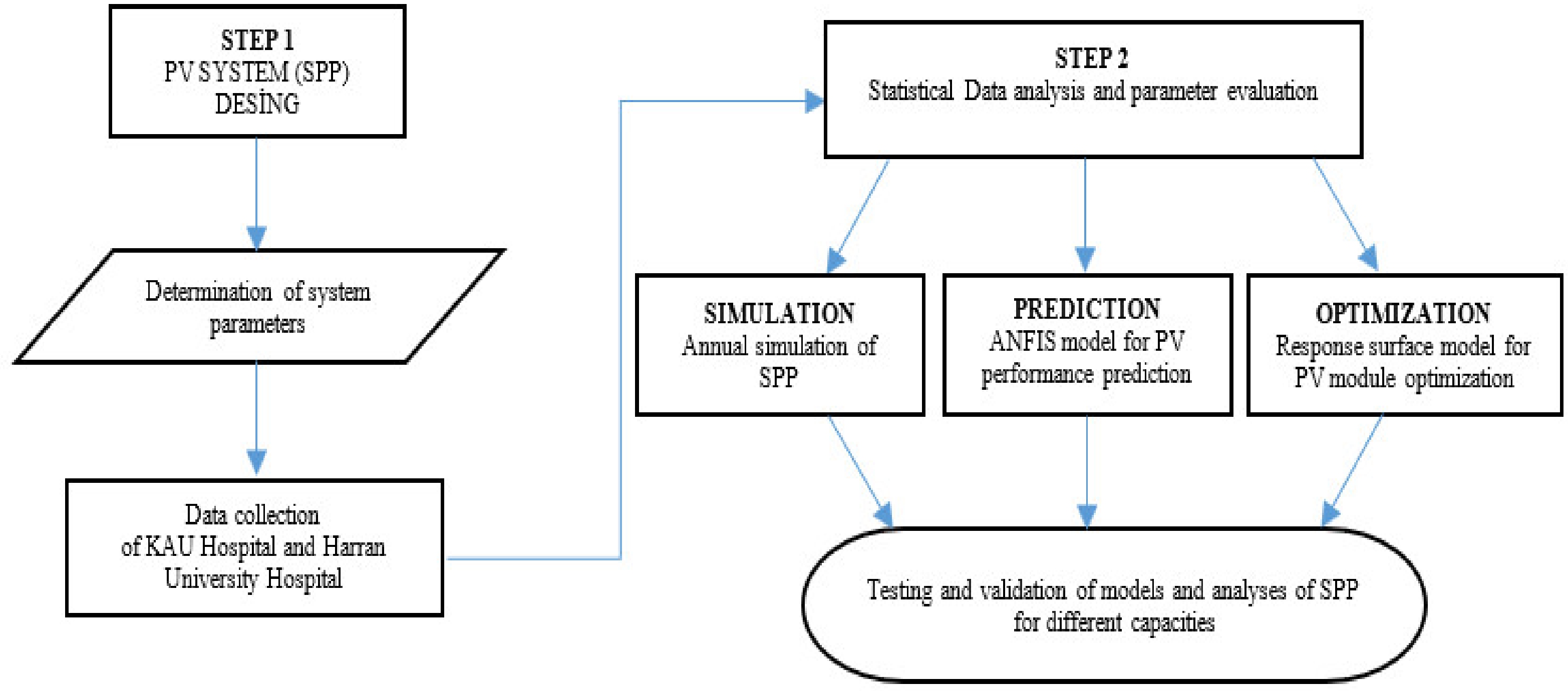
This study aims to design a solar PV system for generating the electricity need of King Abdulaziz University (KAU) Hospital in Jeddah city. The hospital’s energy demand is very high, and the energy consumption bill is around $1.5 million per month. Initially a detailed field work was conducted to determine the PV system performance for self-consumption and self-sufficiency models under real operating conditions. A two step work was carried out: in the first step, a 40 MW PV system was constructed to generate the electricity need of the KAU hospital. The second step includes determining the optimal operating conditions by RSM and ANFIS approaches. Both approaches were employed using the following parameters: surface temperature (°C) of modules, wind speed (m/s), radiation (W/m2), outdoor temperature (°C), and wind direction. The RSM aimed to find out the optimal operating conditions of the solar PV panels and the factor space operating intervals required for the PV panel system. Our investigations depicted that generating maximum solar PV of 42.27 MW is possible for the KAU hospital, if the radiation level is about 896.3 W/m2, the module surface temperature is 50.0 °C, the outdoor temperature is 40.3 °C, the wind direction is 305.6 and the wind speed is 6.7 m/s. On the other hand, the operation conditions of solar PV panels were simulated under different conditions, for instance, it was determined that obtaining a 33.96 MW solar PV system, the radiation should be 896.3, the module surface temperature should be 43.4 °C, the outdoor temperature should be 40.3 °C, the wind direction should be 305.9 and the wind speed should be 6.7 m/s.
The ANFIS intended to develop and analyze the solar PV modules by estimating the performance of them. The ANFIS models developed for the PV generation system can predict the performance of modules containing five, nine and eleven rules. Figure 1 presents the flow chart for this study including the solar power plant (SPP) design procedure and the applied methods.
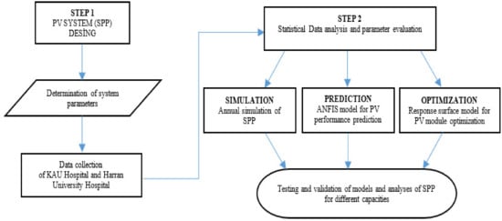
Figure 1.
The solar PV panel system flow chart.
Thus, the design of this study is as follows; in Section 2, the solar PV system design is explained. Simulation of the solar PV system is discussed in Section 3. The data related to solar PV system parameters are analyzed, additionally, the performance prediction and optimization methods; the RSM and ANFIS approaches are given in Section 4. Section 5 covers the results, finding and discussions for the PV system. Section 5 is devoted to the conclusions.
2. Materials and Methods
2.1. Solar Energy Generation Design for KAU Hospital
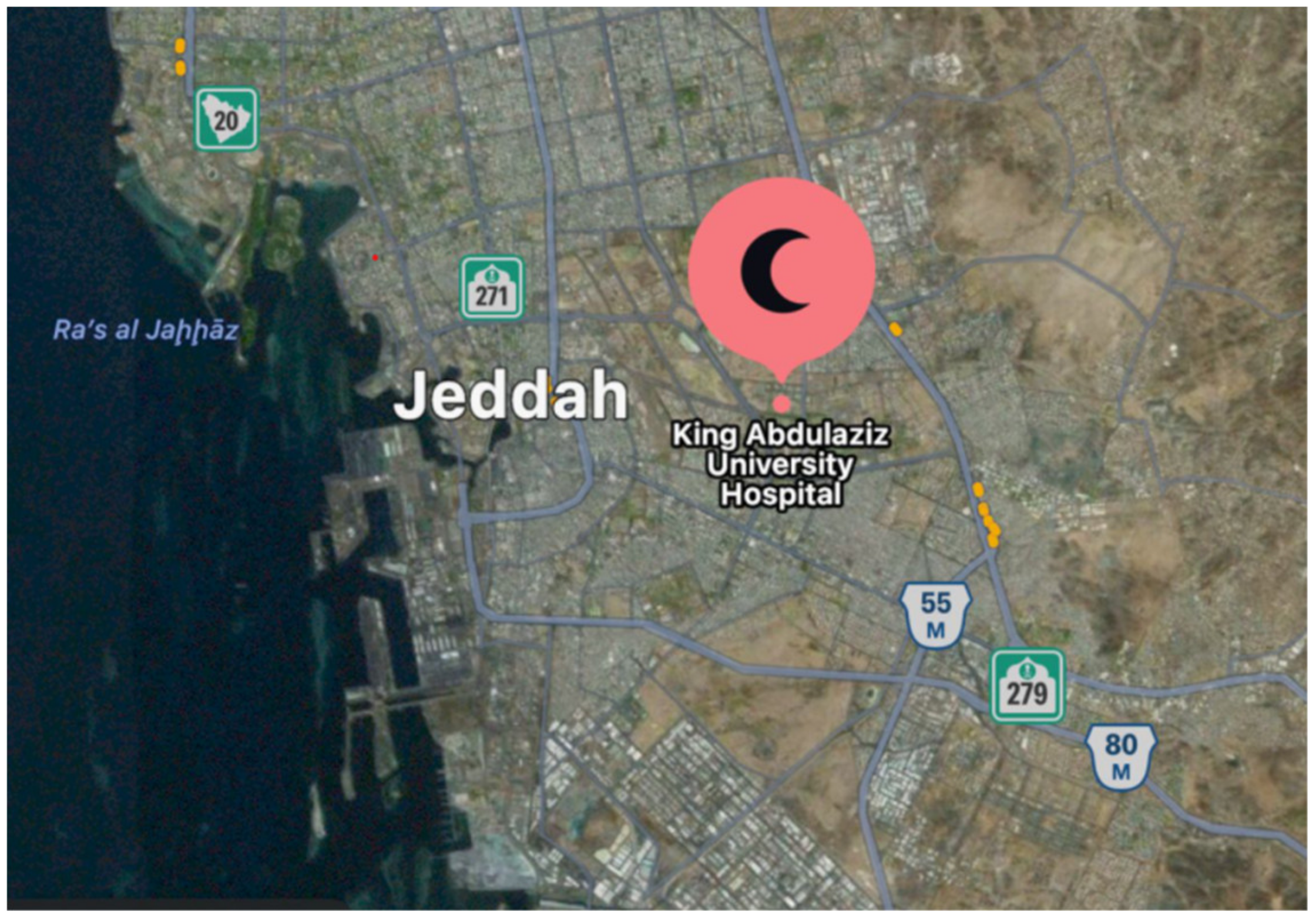
The aim of this study is to construct a solar power plant (SPP) system to generate electricity for KAU Hospital. The hospital is in the KAU campus, the coordinates are [Lat/Lon] 21.290 and 39.130, as shown in Figure 2.

Figure 2.
Location of the KAU hospital.
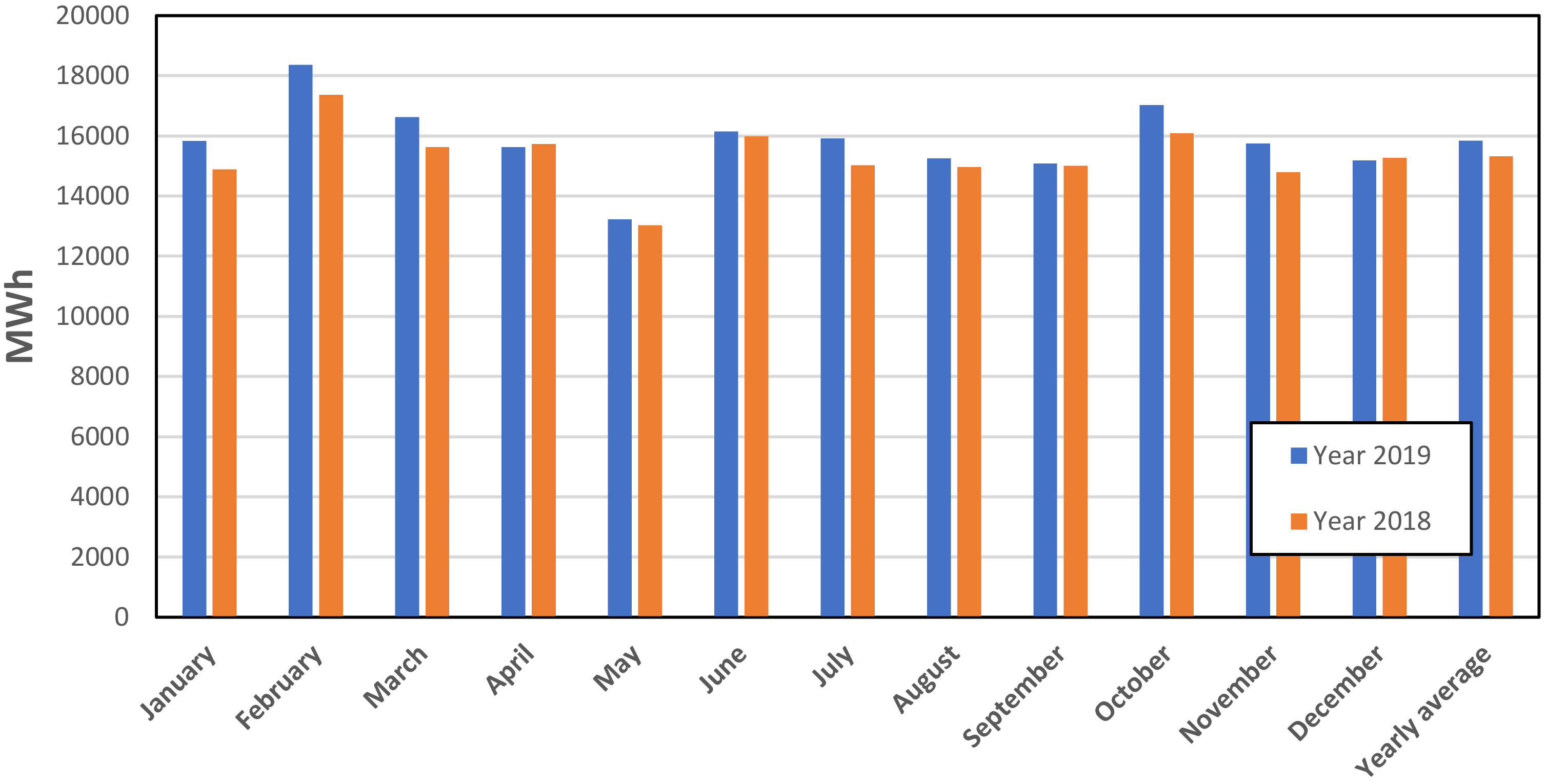
The hospital has a very high electricity consumption. Monthly electricity consumption data of KAU hospital for 2018 and 2019 are given in Figure 3. The maximum energy consumption of the hospital is during February, and the minimum consumption is in May. When the data of 2019 are analyzed, the annual average hourly electricity need of KAU hospital is determined as 21.694 kWh.
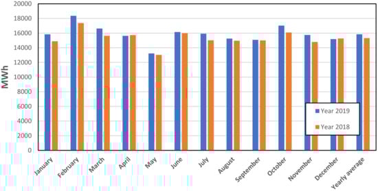
Figure 3.
Monthly electricity consumption of KAU hospital.
2.2. The Solar Power Plant Types
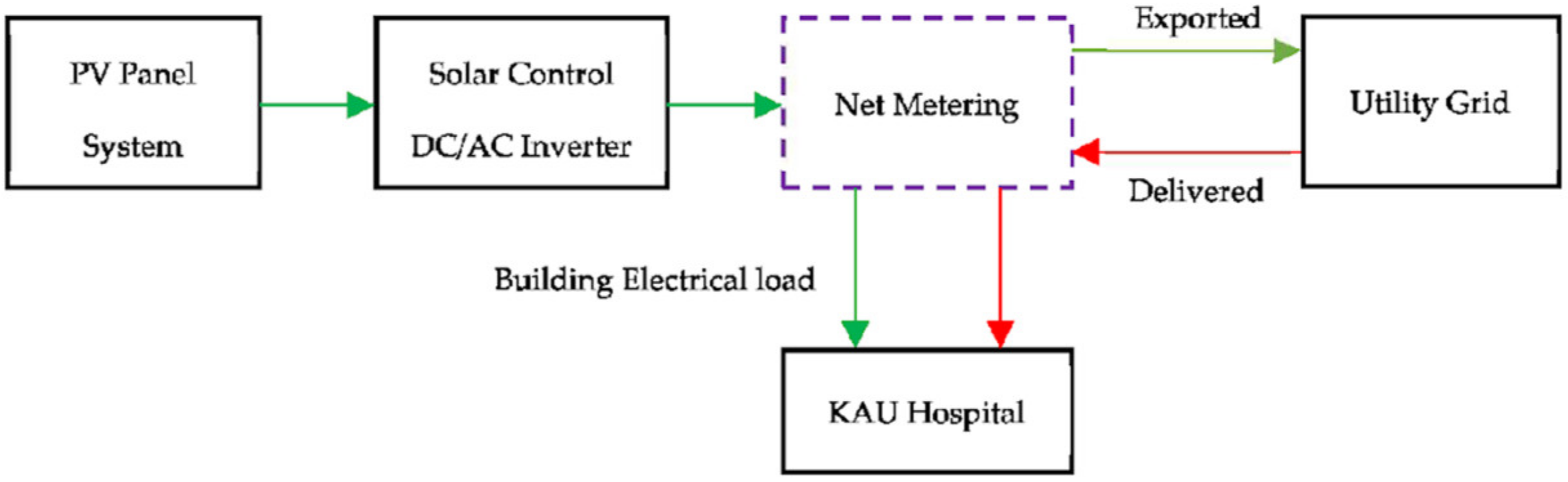
The schematic picture of the PV solar system designed for the hospital is given in Figure 4. The system proposed for the hospital is an on grid PV system. While the sun is available during the day, the electricity need of the hospital will be met by generating electricity from solar energy. This model is known as a self-consumption model and was established to meet the electricity needs of a hospital. These models are called self-sufficient models. If the capacity of the system is well designed, which means greater than the energy consumption of the hospital, the excess energy can be supplied to the national grid during the daytime and reused at night.
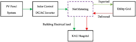
Figure 4.
On grid solar power system for KAU hospital.
In this study, the PV system was designed according to the self-consumption model approach without storing the energy generated, and then the system’s self-sufficiency values in different capacities were found. At the end of the study, the optimum capacity of the PV system was determined for different self-sufficiency rates.
2.3. PV System Design
This study aimed to find the hourly electricity consumption values by using the monthly respective data set of the KAU hospital. Additionally, the data obtained from Harran University hospital (HUH) in Sanliurfa, Turkey, were employed for model building because the energy consumption of HUH is met by the SPP in accordance with the self-consumption model. In SPP of HUH, the electrical energy generation and consumption values of the hospital, and the local meteorological data are measured and recorded every 5 min. In this study, the electricity consumption (electricity load) profiles of both hospitals were considered equal by benchmarking the parameters. The PV system has been designed to perform the following steps:
2.3.1. Determining the Hourly Distribution of the Energy Consumption of the Harran University Hospital
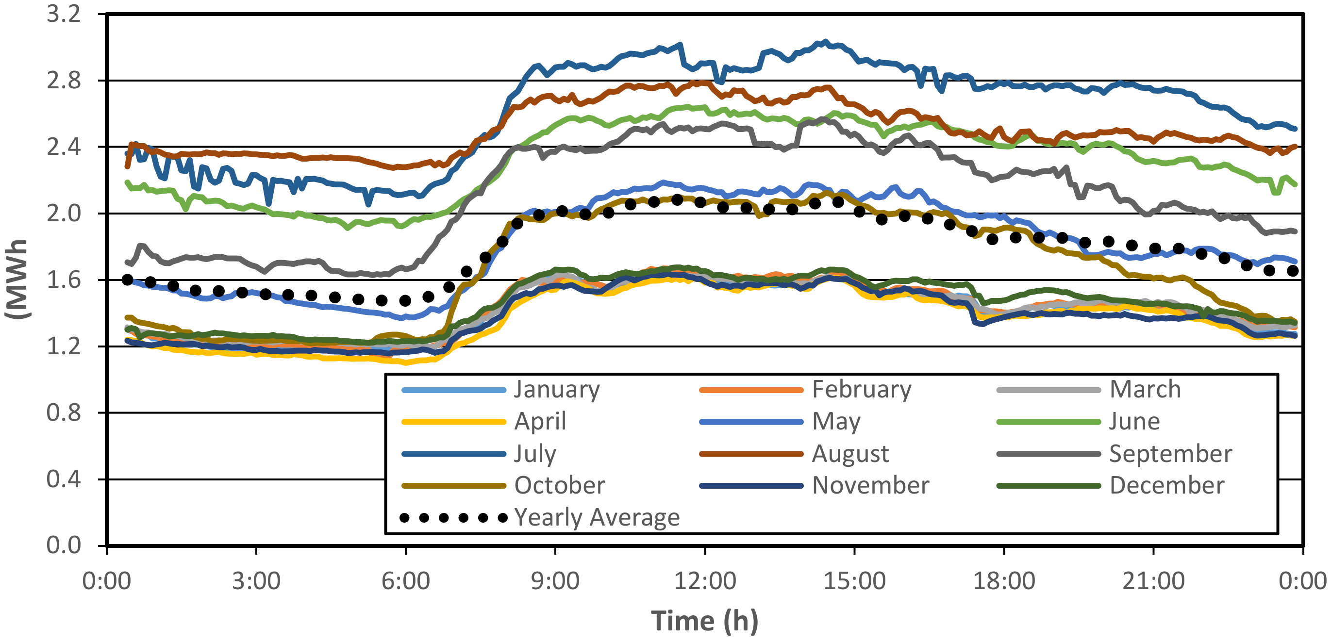
Using electrical energy consumption of HUH between 1 January 2019 and 31 December 2019, hourly energy consumption was determined for an average day of the month. In Figure 5, according to the monthly and annual data of HUH, the distribution of electricity consumption for an average day is given. As can be seen from Figure 5.
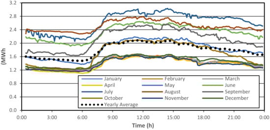
Figure 5.
Monthly and yearly average distribution of the electricity consumption of Harran University hospital.
- The maximum energy consumption of HUH is in July.
- Electricity consumption is the highest in 4 months (summer period) from June to September,
- Electricity consumption is the lowest in the period of 6 months (winter period) from November to April,
- The electricity consumption profiles of an average day obtained for May and October are similar to the consumption profile obtained for an average day determined according to annual data.
2.3.2. Determining the Load Profile of the Energy Consumption of the Harran University Hospital
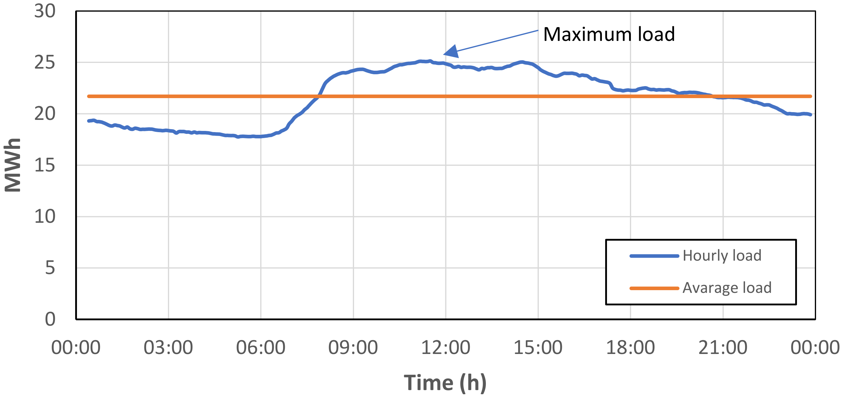
The electrical energy consumption load profile (LR) of HUH was calculated according to the following equation. In this equation, it shows hourly electrical energy consumption value with Qhour and annual/monthly average hourly energy need with Qaverage. According to the 2019 data of HUH, the daily average electrical energy consumption profile for 2019 is presented in Figure 6.
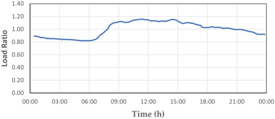
Figure 6.
Average daily electrical energy consumption profile of Harran university hospital for 2019.
2.3.3. The Hourly Energy Consumption Distribution of the KAU Hospital
The electricity consumption profiles of two hospitals are considered similar. Considering the daily electricity consumption profile of HUH, and the hourly electricity consumption distribution profile, and the monthly total energy consumption values of KAU hospital, the average hourly energy requirement (Qhour) of KAU hospital was calculated according to following equation:
According to the consumption data in 2019, the KAU hospital’s (Figure 3) hourly electricity requirement is 21.694 kWh on average. The daily electricity consumption profile of the hospital is presented in Figure 7. This figure shows the maximum electricity requirement of KAU hospital which shows that it is 25.135 kWh at 11:30. If the PV system is designed according to the maximum electricity requirement of the KAU hospital, a PV system with 25 MW of capacity should be sufficient. However, in real operating conditions (local climatic conditions) PV panels perform with lower efficiency than their efficiency stated in the catalogue because of high temperature. PV panels are tested under 1000 W/m2 solar radiation and 25 °C outdoor temperature conditions.
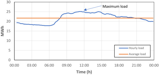
Figure 7.
Daily average electrical energy consumption profile of KAU hospital.
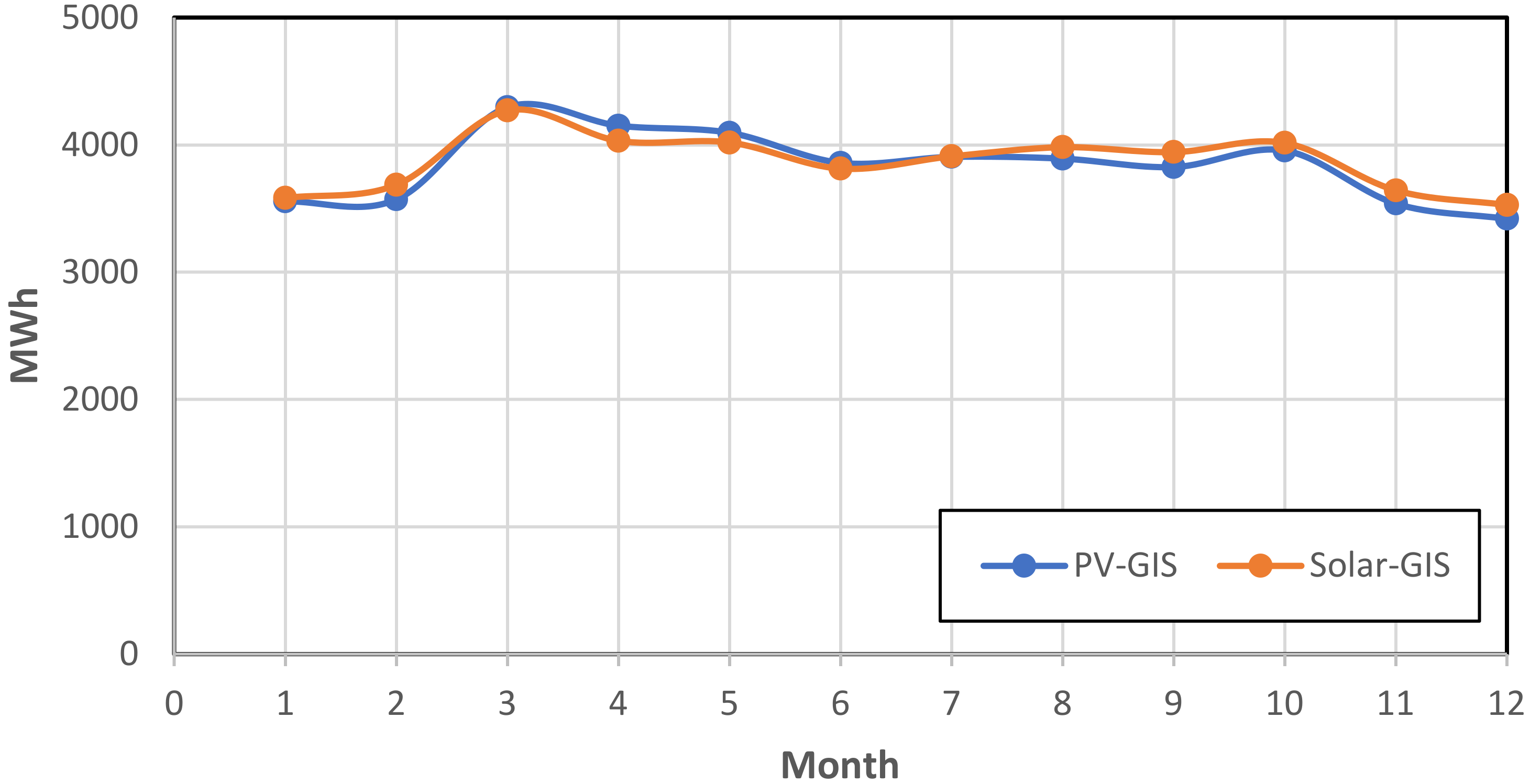
PV system designing in accordance with the self-consumption model (according to the hourly electricity consumption need) aims to meet the electricity needs of KAU hospital. To meet up the electricity needs of KAU hospital, an on-grid PV system of different capacities, ranging from 25 MW to 100 MW, was designed. Thus, performance evaluation of PV systems designed for different capacities was made easy. In all PV systems, crystalline silicon technology was used. PV panels are mounted and fixed in the open area to face them to the optimum tilt angle of the south direction. The optimum tilt angle for Jeddah is 22 degrees. Total losses of the PV system (inverter, cable, dust, etc.) were considered as 14%. In this study, all PV designs determined for KAU hospital were simulated under the local climate conditions of Jeddah and detailed analysis was carried out. For PV system simulation, the Solar-GIS program [39] was used. The PVGIS program [40] was used to validate the simulation results obtained from the Solar-GIS program which are the online ideal free tools that can be used for estimating electricity generation of the PV system. In Figure 8, the monthly electricity generation values obtained by both PVGIS and Solar-GIS programs of the PV system with 25 MW capacity are compared. The results obtained from both programs are very close to each other.
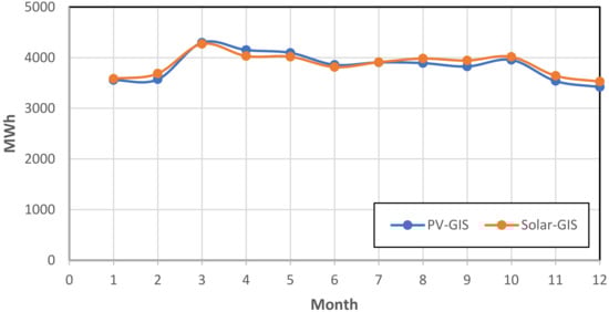
Figure 8.
The comparison of monthly electricity generated from both PV-GIS and Solar-GIS programs for a 25 MW PV system.
3. Solar PV System Analysis and Performance Prediction
3.1. Data Collection and Analysis
Determining the optimal performance of the solar PV generation plant, precise and truthful parameters were ascertained, and related data were collected. The data employed in this study are for the time duration from January 2019 to December 2019 of radiation (W/m2), module surface temperature (°C), wind speed (m/s), outdoor temperature (°C), and wind direction which were gathered from Harran University solar power plant located in the university campus. Wind direction measurement is expressed with an angle showing 0° of the north, 90° of the east, 180° of the south and 270° of the west. Historical data for the (37.158/39.007) [Lat/Lon] of variabilities of solar resources were obtained from monitoring stations located in Sanliurfa, Turkey. A comprehensive statistical analysis was conducted to determine the multicollinearity to show the intercorrelation between the independent factors. The findings showed that the module surface temperature and outdoor temperature are highly related to the remaining independent variables. The ‘P, F, t and VIF’ tests indicated the availability of redundant information among the independent variables, and weak linear relations, the interactions of predictors may be nonlinear, and the nonlinear relations can be dealt with RSM, ANFIS and simulation approaches.
Truly, there is often no unique ‘best’ set of independent variables that can be said to yield the most excellent outcomes. Different techniques do not all automatically lead to the same final prediction of related variables. As a result of the fact that the variable selection process is sometimes subjective, analysts may therefore need to emphasise their judgments on the pivotal areas of the problem. In this study, the highest coefficient of determination (R2) was found 0.946 for several combinations of sets of independent (input) variables. One interesting combination of the input variables was the radiation, module surface temperature and outdoor temperature. The other combination was the addition of all parameters for model development, both giving 0.946 coefficient of determination ratio. Therefore, we used all five parameters for ANFIS model development.
3.2. RSM for Optimization of Solar PV System
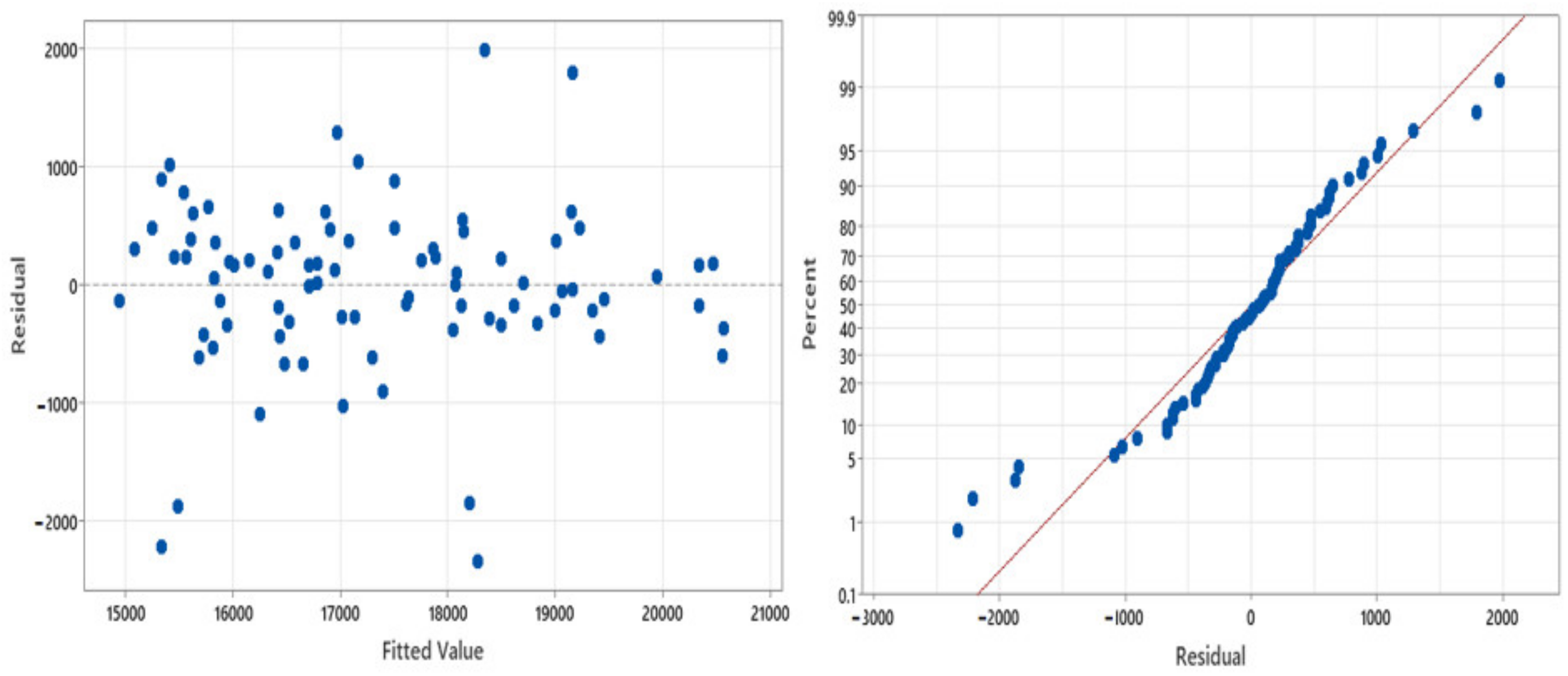
RSM is an optimization method used to determine the operating conditions of a process leading to achieving the best process performance [41]. RSM has extensive applications in semiconductors, electronics manufacturing, and machining. In most RSM problems, the form of relationships between independent factors and response is assumed unknown. When there are curvature relations between the factors in a system, a higher degree polynomial of process optimization approach can be employed, such as a second order model or above. Obviously, a polynomial model is unlikely to be a reasonable estimate of the true functional relationship over the entire domain of independent parameters, but for a relatively small region, the method works quite well. Figure 9 shows that there is no serious indication of the abnormality or excessive evidence of possible outliers. This plot also reveals nothing of unusual interest among the residuals, and the residual scatter does not appear more for the outcomes that show nonhomogeneous conditions. Therefore, the model is assumed to be adequate, the investigation of the normality assumption also approves the adequacy.
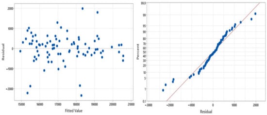
Figure 9.
The probability plot of solar PV generation response, and the dispersion of residual.
The regression equation of solar PV generation where the factors are radiation (x1), module surface temperature (x2), outdoor temperature (x3), wind direction (x4) and wind speed (x5) were established according to the following equation.
where βjj, represent the overall mean effect, the effect of the j-th level of the row factor, the effect of the j-th level of column factor, and the effect of the interaction effect in the quadratic model, respectively. is a random error component of a second order RSM, where is the response and refers to the solar PV generation level in this study. xi and xj present the variables that are called factors. Dirnberger and Kraling (2013) [42] described the measurement procedure and uncertainty analysis which covers the complete daily calibration process of measurement devices in detail, the correction to standard testing conditions, and determination of electrical module parameters. They presented recent progress in reducing the measurement uncertainty for crystalline silicon and thin-film PV modules.
The essential effects that arise from this analysis are the key impacts of x1, x2, x3, x4 and x5. The interactions between the parameters x1 x2, x1 x3,… are presented in the regression model with the coefficients presented above in the model.
3.3. ANFIS Approach for PV Efficiency Estimation and Analysis
The ANFIS model comprises ANNs and fuzzy logic to forecast the output data identified by input parameters. An ANFIS model is constituted by membership functions (MFs) [15]. Higher MFs numbers usually affect the outcomes optimality with lower accuracy [43], additional MFs cannot improve the effectiveness of a fuzzy model [44]. A fuzzy model’s performance depends on efficiently selected system parameters, their complexity, and the type of training algorithm called the ANNs [45,46,47,48].
An ANFIS includes fuzzy implications presented in fuzzy ‘If-Then’ rules to represent the relations of fuzzy inputs-outputs parameters linguistically [15]. An efficient parameter control depends on the number of rules. In other words, an ANFIS is shaped by fuzzy rules and their term sets [46]. The rules are the backbone of an ANFIS system. When the parameters are nonlinear, Gaussian membership functions are used for identifying the fuzzy terms which will be used to forecast the PV generated. The aim of an ANFIS model is to forecast the performance of the solar PV module. The set of input–output data was split into three randomly selected parts: training data, testing, and validation data. Training data set includes 319 observations served for the ANFIS model building, and for testing and validation 100 data were employed, respectively. The designed ANFIS model consists of five nodes for input parameters with 25 Gauss membership function, five nodes in the hidden layer (H1~H5), and a node (Pk) to show the solar PV model outcome for the output layer. Hence, the ANFIS model has a total of sixty eight nodes arranged with thirty linear and fifty nonlinear parameters corresponding to the five input parameters.
The input parameters of ANNs are the radiation (W/m2; x1), module surface temperature (°C; x2), outdoor temperature (°C; x3), wind direction (x4), and wind speed (m/s; x5) and the outcome parameter of network is the PV generated (Pk). The input-hidden and hidden-output layers’ coefficients called weights are presented by and , correspondingly. The following equation was used to calculate the k-th neuron’s outcomes in the hidden layer.
The input variables’ MFs is shown by , , depicts the weighting coefficient in the hidden layer. shows the output MFs in the hidden layer and is found according to the following equation.
where f(net) is the activation function in ANNs and the following equation was used to determine it.
where m and show the number of neurons in a hidden layer and the weights, respectively. For the training process, input data were used, the outcomes of ANFIS model were determined and compared with the actual (Ak) outcomes presented in Equation (8). The learning constant value η was set up as 0.25, 0.50, and 0.70 as given in the following equation.
The best outcome of learning constant was obtained when η is equal to 0.70. The error of the p’th observation can be calculated according to the following equation.
The number of training data N, actual outcomes (Ak) and the predicted outcomes (Pk) are presented in the equation given above. The (E) shows the error estimator, is a squared error minimization function and called the Least-Squares Estimator (LSE). For specifying Gaussian membership functions (MFs), two parameters (c, σ) are used; the center ‘c’ of MFs and the width ‘σ’ of MFs are used for identifying the MFs.
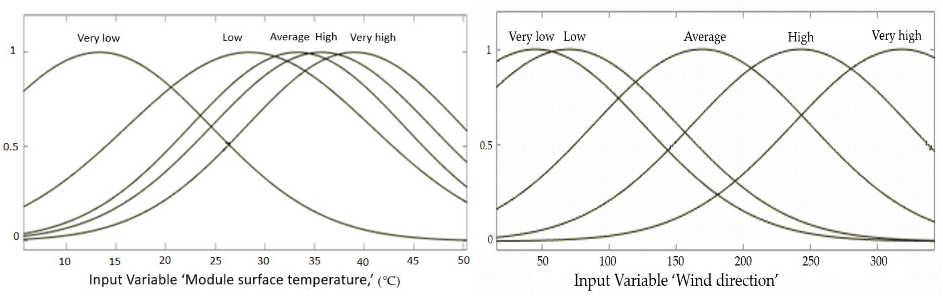
The Gaussian MFs are shown in Figure 10 for the input parameters ‘wind direction’ and the ‘module surface temperature’, respectively. Their fuzzy linguistic term set can be stated as {very low, low, average, high, and very high}. The MF can be presented with a mathematical relation conforming to the following equation for the fuzzy linguistic term ‘average’ for the wind direction.
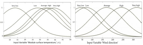
Figure 10.
Gaussian MFs for wind direction and module surface temperature.
The fuzzy membership function of the fuzzy term ‘average’ used to identify the factor ‘wind direction (x4)’.
A neuro-fuzzy model is a set of fuzzy ‘If-Then’ rules [47]. Sugeno fuzzy modelling approach suggests an efficient way to produce fuzzy rules from the parameters data. In a Sugeno fuzzy model, fuzzy rules are usually constituted in the following form. In the following equation, B and C are the antecedent of the fuzzy term sets, whereas yn = fn(x1, x2,…, xm) is the consequent part of the fuzzy rule. The input parameters (x1, x2,…, xm) are depicted as polynomial functions fn(x1, x2,…, xm), and rn is the constant, presented as follows:
IF x1is B and x2is C …… THEN yn = fn(x1, x2,…, xm) = bnx1 + cnx2 + dnx3 + …knxm + rn
The fuzzy reasoning procedure produces crisp outputs, ‘y’ shows the amount of PV generated under certain conditions by the modules. Thus, a fuzzy rule set of input–output parameters of a PV energy generation plant can be presented as follows.
Rule 1.
IF ‘The radiation is 249 (W/m2) and the module surface temperature is 28 °C AND the outdoor temperature is 31.2 °C AND the wind direction is 180. AND the wind speed is 2.92 m/s THEN The amount of PV energy generated is (kWh) = 4.575x1 − 14.39x2 + 14.13x3 − 0.0469x4 − 6.22x5 + 339.4934 (1490 kWh).
Rule 2.
IF ‘The radiation is 336 (W/m2) and the module surface temperature is 26.7 °C AND the outdoor temperature is 15.6 °C and the wind direction is 134. AND the wind speed is 3.22 m/s THEN The amount of PV energy generated is (kWh) = 6.785x1 − 65.26x2 + 25.35x3 − 0.574x4 − 67.35x5 − 275.995 (363 kWh).
The ANFIS model for the solar PV generation was developed using 319 data for training, 100 for testing, and 100 for the validation of the model. The training errors were determined for the observations by differencing the actual data (At) and the predicted data (Pt) obtained from the solar PV fuzzy inferencing model. The ANFIS model was optimized during the training process, and several factors were arranged to obtain the best outcomes. The optimization of ANFIS model and training process depend on certain factors such as the range of influence was set to 0.7, so the squash factor set to 1.25, the accept ratio set to 0.75 and the reject factor was set to 0.157 in this study. Additionally, the error tolerance limit was arranged as 0.001 and epochs as 3000. Consequently, the Root Mean Square Error (RMSE) achieved 66.98 for the training process of ANFIS model with nine rules, 113.5208 for ANFIS model with five rules, and 68.47 for the ANFIS model with eleven rules. On the other hand, the training error can be recorded as the mean squared error (MSE) for a trained ANFIS model. The MSE was calculated as follows:
To minimize the training process error, the gradient vector is obtained initially, calculated from the output layer by derivation of the findings and propagating backward until the input layer. In this work, three ANFIS models were developed including 5, 9 and 11 rules based on the sub clustering algorithm. Considering the training error and RMSE, the ANFIS model having 9 rules gave the best outcomes with minimum error for the solar PV generation model examined. The error (residual) was determined 0.5362% for the solar PV generation model of 9 rules ANFIS model, 1.26% for the ANFIS with 5 rules and 1.082% for the ANFIS model that has 11 rules. On the other hand, the performance of the ANFIS models was tested based on different rule-bases of the solar PV system. The findings are assessed and compared with the other models using the average prediction error approach. The following equation was employed for the calculation of the average prediction error.
4. Results and Discussions for Solar PV System Findings
4.1. The Assessment of PV System Simulation
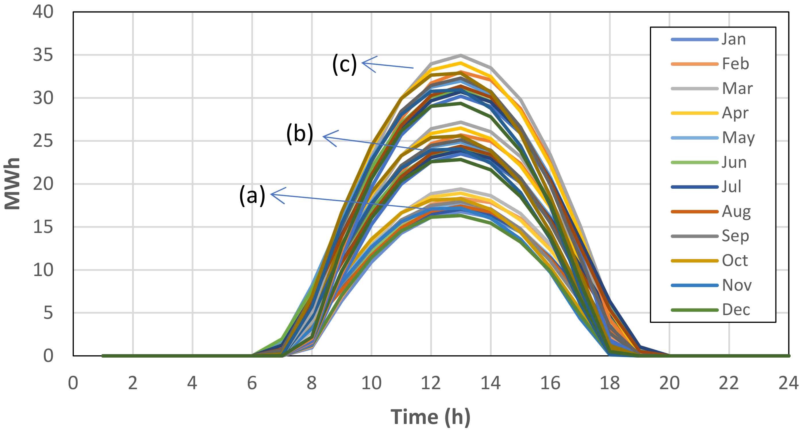
According to the results of the simulation of the PV system, yearly average values of PV electricity (AC) delivered by the total installed capacity of a PV system were found to be 1843 kWh/kWp. Figure 11 shows the distribution of hourly electricity production values of the designed PV systems by all months. As seen in Figure 11a, the system capacity is 25 MW and the maximum monthly electricity production is between 16 and 19 MWh. The maximum electrical energy requirement of KAU hospital will be approximately 25 MWh. The energy generation amount of the PV system for a capacity of 25 MW was less than the hourly electricity requirement of the hospital. As seen in Figure 11b, when the system capacity is 35 MWh, the maximum electricity generation is approximately in the range of 23 to 26 MWh. Therefore, it cannot meet the hourly energy needs of the hospital in some months. Figure 11c shows that the system capacity is 45 MW and there is an exceeding production level of the hourly maximum electrical energy requirement of the hospital in all months. In case the electricity produced from the PV system is more than the electricity consumption of the hospital, the excess production is given to the local electricity grid (on grid PV system). When there is no production of the PV system, the electricity need of the hospital is met by the local electricity grid.

Figure 11.
Average hourly profiles of total photovoltaic power output for; (a) 25 MW of PV capacity, (b) 35 MW of PV capacity, (c) 45 MW of PV capacity.
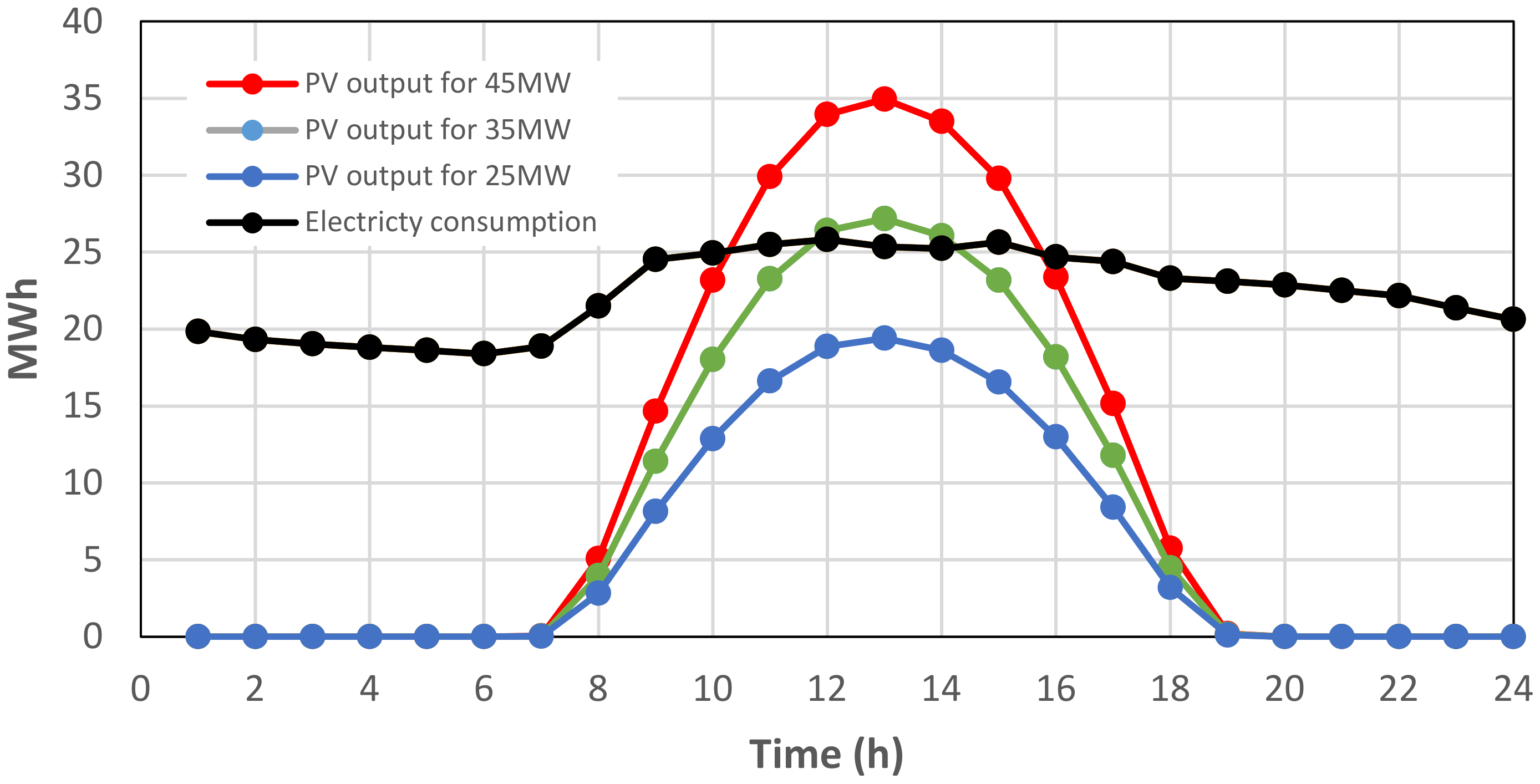
In all PV designs, the highest electrical energy production during the year was determined in March. The daily distribution of electrical energy production values of all PV systems in March are shown in Figure 12. In addition, the graphs show the hourly electrical energy consumption profile of the hospital for an average day of 2019.
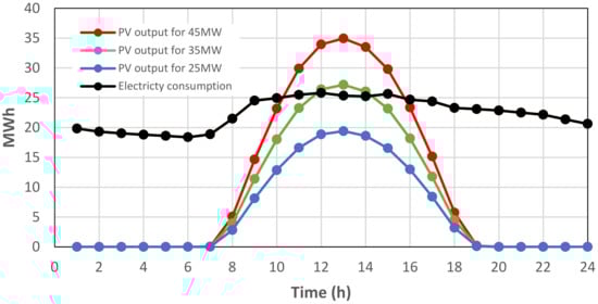
Figure 12.
Average hourly profiles of total photovoltaic power output in March for 25 MW of PV capacity, 35 MW of PV capacity and 45 MW of PV capacity.
As seen in Figure 12, when the system capacity is 25 MW, the maximum electricity generation is approximately 20 MWh. The energy generation capacity of the PV system with 25 MW is below the hourly electricity requirement of the hospital. On the contrary, as it is seen in Figure 12 when the system capacity is 35 MW, the maximum electricity generation is approximately 27 MWh. The PV system produces the electrical energy needs of the hospital between 12:00 and 14:00 h. The PV system of 45 MW capacity can meet the electrical energy requirement of the hospital between 10:00 and 16:00 h, and some extra energy is produced.
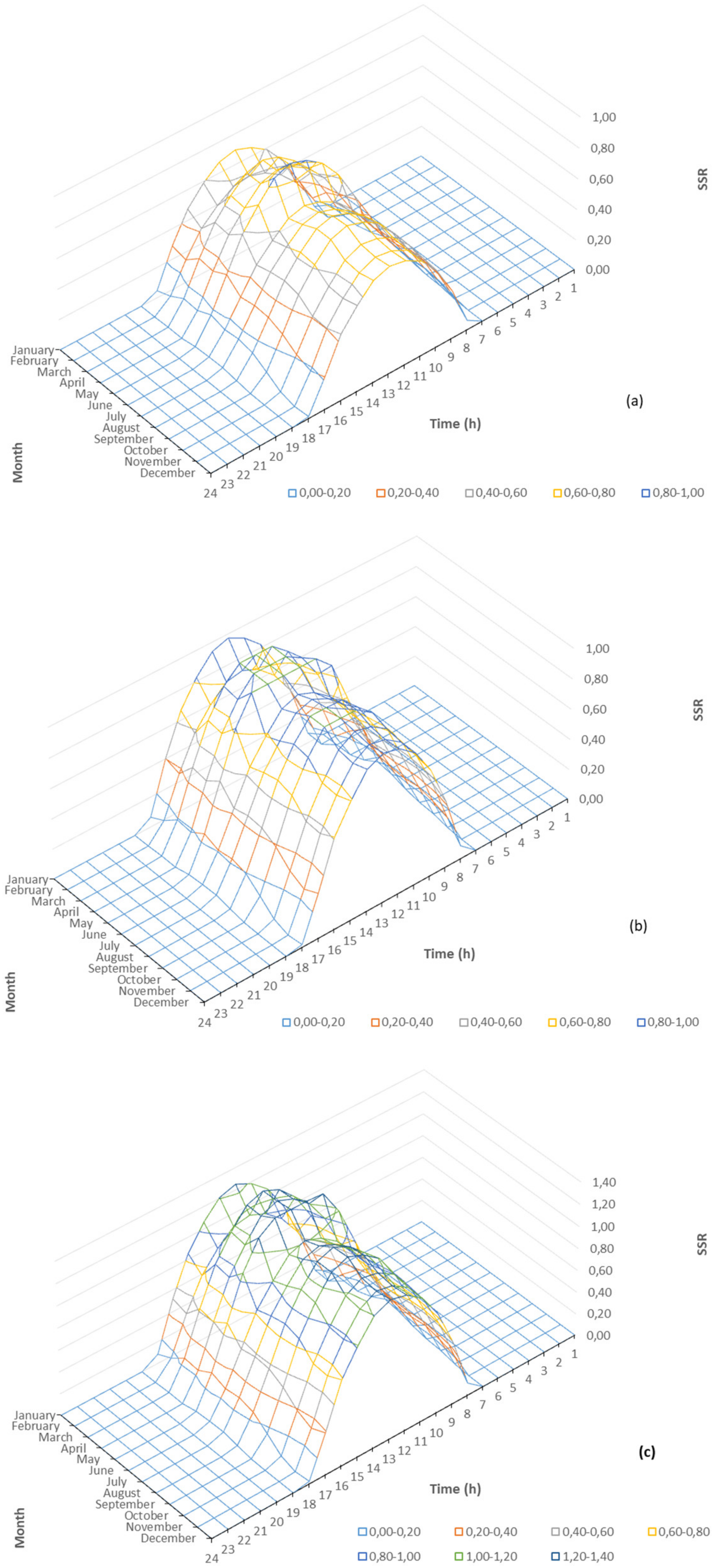
Figure 13 shows the ratio of meeting the hourly electricity requirement of the hospital with energy generated from the PV system by all months. This ratio is called the self-sufficiency value of the PV system. For example, if the self-sufficiency ratio (SSR) is 30%, it means that 30% of the electrical energy requirement is produced from the PV system. On the other hand, self-consumption indicates that the entirety of the energy produced from the PV system is consumed instantly. This system does not have any storage units and are not fed to the local electricity grid. As it is seen in Figure 13, the self-sufficiency profile is similar in all capacities. Among the distribution of SSR data by month, the lowest performance was observed in February, but the highest performance was observed in May.
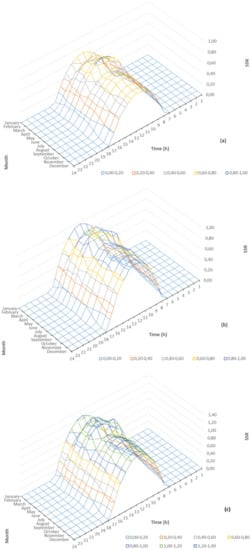
Figure 13.
The ratio of PV systems meeting the hourly electricity need of the hospital (a) 25 MW of PV capacity, (b) 35 MW of PV capacity, (c) 45 MW of PV capacity.
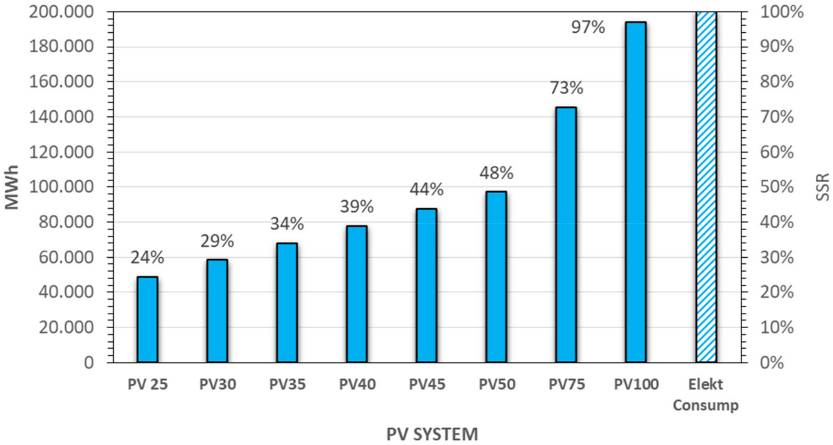
Table 1 presents the self-sufficiency ratio of PV systems for monthly and yearly periods. The highest performance was observed in May and this ratio was 31% for PV25, 37% for PV30, 43% for PV35, 50% for PV40, 56% for PV45, 62% for PV50, 93% for PV75 and 124% for PV100. According to the annual simulation results given in Table 1, the self-sufficiency ratio of the PV system for the KAU hospital is found as 24% for PV25, 29% for PV30, 34% for PV35, 39% for PV40, 44% for PV45, 48% for PV50, 73% for PV75 and 97% for PV100.

Table 1.
Self-sufficiency ratios of PV systems.
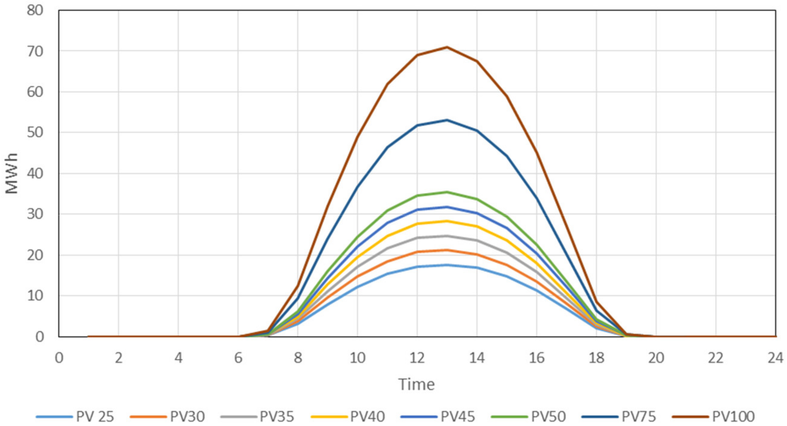
The annual total electricity consumption value of the KAU hospital for 2019 was 190.042.560 kWh. Figure 14 shows the annual electricity generation distribution of PV systems with different capacities for an average day.
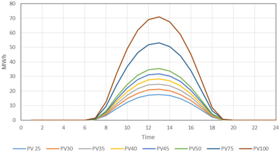
Figure 14.
The annual distribution of electricity generation of PV systems for an average day.
Figure 15 presents the total annual electricity generation of the PV systems, and its comparison with the annual total electricity consumption of the KAU hospital. SSR is also given as a percentage in Figure 15. When the simulation results are analyzed, it is determined that the PV system capacity is 40 MW according to the self-consumption model for the KAU hospital. Based on this self-sufficiency model, the capacity of the PV system is considered 100 MW.

Figure 15.
Total annual electricity generation of PV systems of different capacities.
The Assessment of Solar PV Module Using RSM Approach
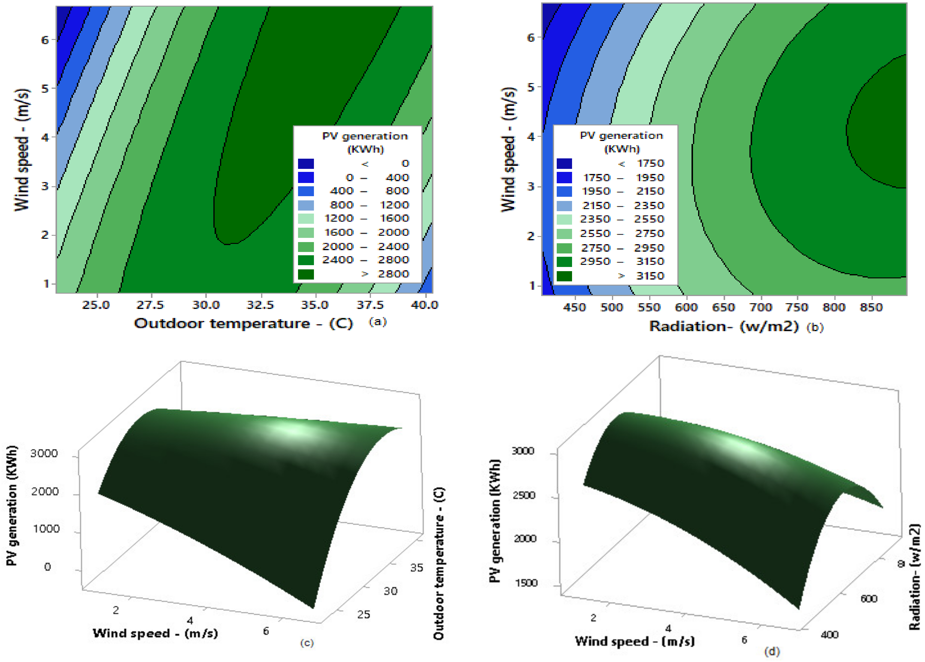
Figure 16a,b show the contour plots of solar PV plants under uncertain conditions. For instance, as depicted in Figure 16a, in case the wind speed is above 2 m per second, and the outdoor temperature is between 30 and 38 °C, the PV yield is 28 MWh. Similarly, Figure 16b shows the contour plots of the PV energy yield, when the wind speed is between 3 and 5.5 m per second and the radiation is above 820 W/m2. Figure 16c,d shows the three-dimensional graph called response surface plot of solar PV energy generation versus wind speed, outdoor temperature, and radiation.

Figure 16.
The contour plot of solar PV generation versus wind speed and outdoor temperature (a) and wind speed and radiation (b). The three-dimensional graph of solar PV energy generation versus wind speed, outdoor temperature (c), and wind speed radiation (d).
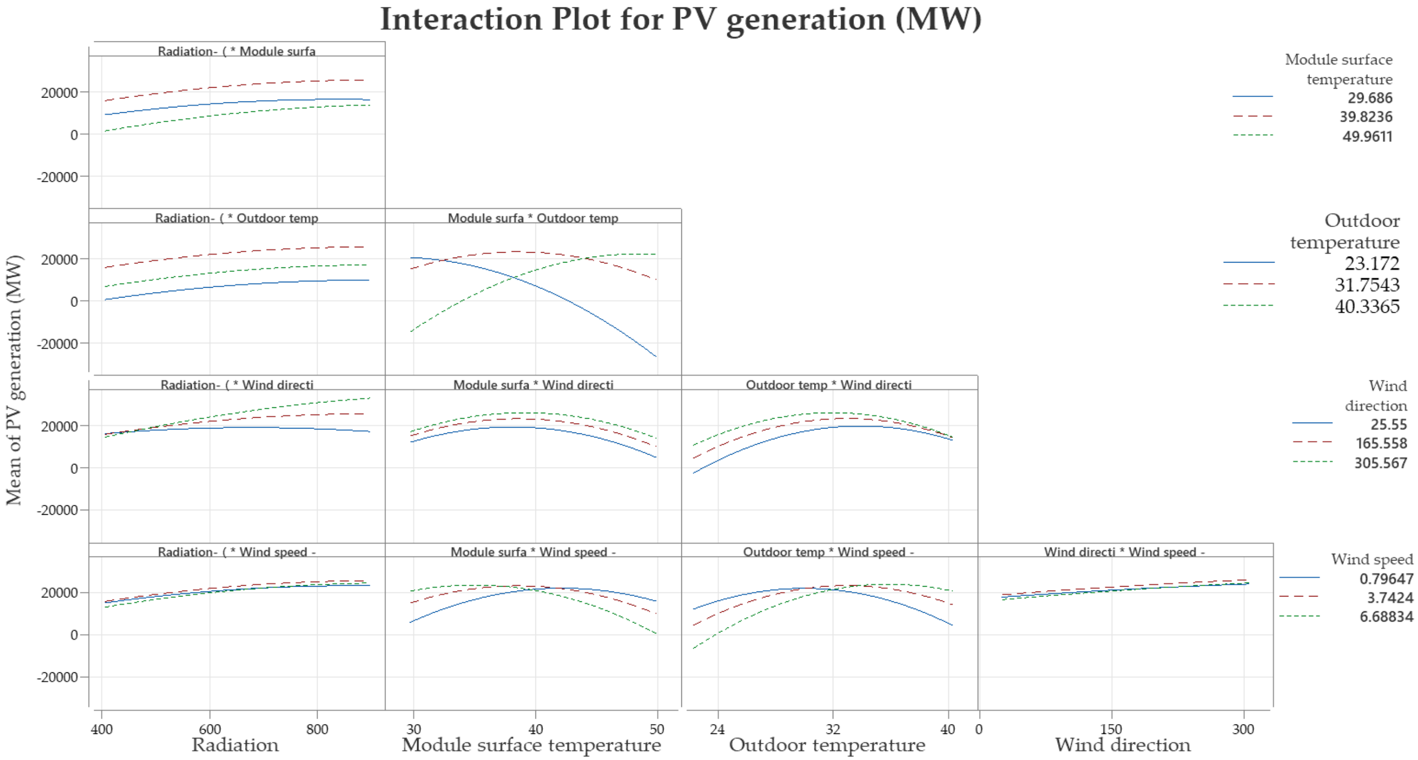
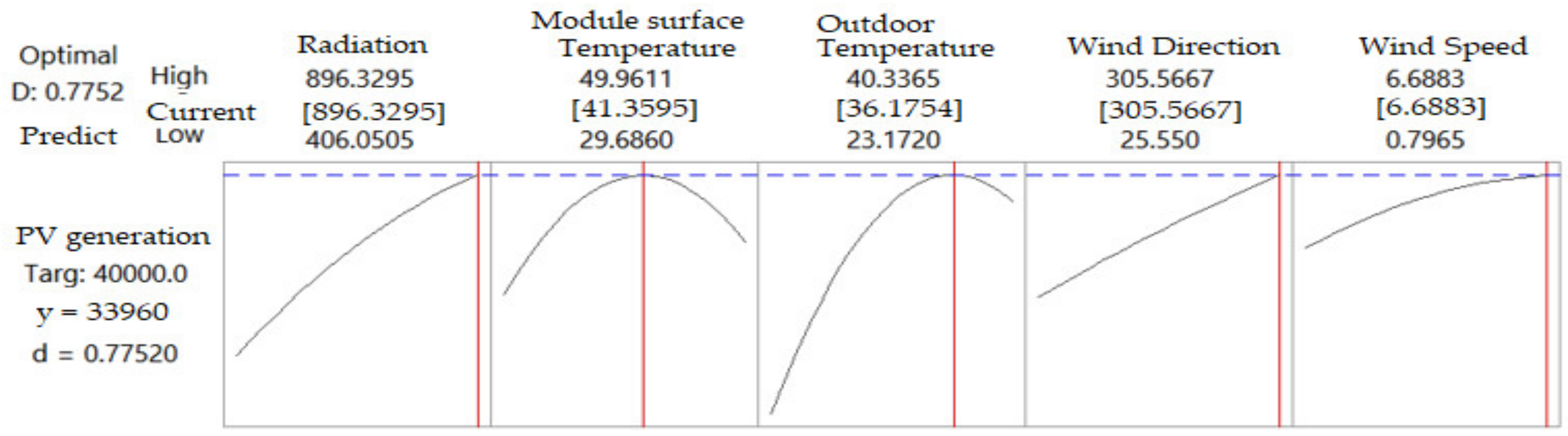
The difference of response is not the same at all levels of the factors in some problems. There is an interaction between the factors. Hence, the parallel lines in Figure 17, indicate, approximately, the factors’ lack of interaction. Therefore, when Figure 17 is examined, the lines seem not to be parallel. This indicates interaction between the factors. In general, optimal solar PV generation is attained at average module surface temperature, high radiation, wind direction and wind speed level. Changing from low to high module surface temperature and outdoor temperature reduce the PV yield. Changing from intermediate to high degree module surface temperature, and outdoor temperature essentially reduces the PV generation. Figure 18 shows the individual effect of factors on the PV system. Hence, optimal PV generation levels of characteristics were determined and presented in Figure 18. Generating maximum PV of 42.27 MW is possible when the radiation level is 896.3 W/m2, the module surface temperature is 50 °C, the outdoor temperature is 40.3 °C, the wind direction is 305.6 and the wind speed is 6.7 m/s.
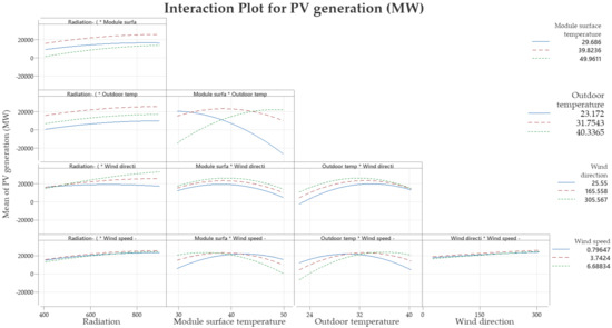
Figure 17.
The plots of independent parameter interaction for solar PV generation.
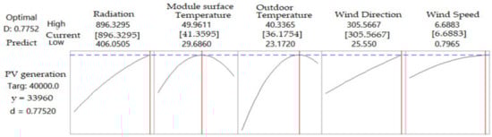
Figure 18.
The individual effect of factors on solar PV generation system.
Figure 18 clearly shows that the intermediate module surface temperature, and outdoor temperature essentially increase the solar PV generation with high radiation, and wind speed. Hence, the optimal solar PV generation characteristics are determined and presented in Figure 18. When the operation conditions of solar PV are simulated under certain conditions, it was determined that the optimal solar PV of 33.96 MW is obtained if the radiation is 896.3, module surface temperature is 43.4 °C, outdoor temperature is 40.3 °C, wind direction is 305.9 and the wind speed is 6.7 m/s.
The effect analysis of the main factors x1, x2, x3, x4 and x5 and the interactions x1x2, x1x3, x1x4 and etc are presented in the regression model. The effects of interactions and main factors showed that four factors positively affect the solar PV generation, only wind direction negatively affected it. Our investigation showed that the coefficients of x1x2, x1, x1x2, x12 and x12 are very small, hence these interactions can be bounded. The effects of interactions and the main parameters are plotted in Figure 17 and Figure 18, respectively. Four effects are positive in this equation, only wind direction has a negative effect. Hence all main effects are only considered to determine the optimal level and maximize the solar PV level.
4.2. The Assessment of Performance of Developed Models Using ANFIS Approach
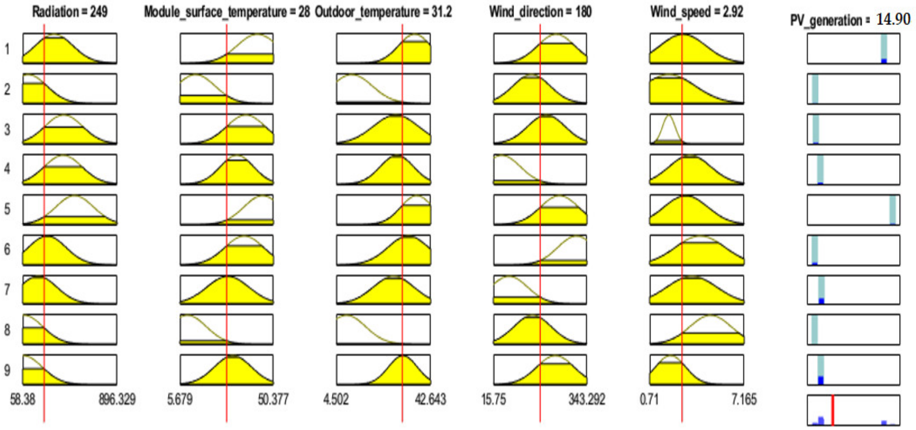
For inferencing and obtaining the outcomes, fuzzy reasoning is used. As appears in Figure 19, fuzzy ‘If-Then’ rules are used for reasoning procedure, a nine rules ANFIS model was developed for the PV energy generation system. As appears in Figure 16, when the radiation is 249 W/m2, the module surface temperature is 28 °C, the outdoor temperature is 31.2 °C, the wind direction is 180 and the wind speed is 2.92 m/s, then according to ANFIS approach, the PV module can generate 14.90 MW power.
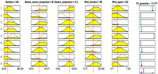
Figure 19.
Fuzzy reasoning for PV energy generation system.
For testing the developed RSM and ANFIS models, the randomly selected input data were used to test the methods and to determine how perfectly they can generate and predict the consequences of the parameters. This step covers testing the performance of RSM and ANFIS approaches for the validation of the models. As appears in Table 2, a large amount of data set was utilized to identify the input–output interactions of the model. The findings of the RSM and ANFIS models for certain input factors are presented in Table 2.
Table 2.
Actual and predicted solar PV generated for certain parameters.
The results and findings showed that the average prediction error of the RSM model was found to be 1.743%. Similarly, the ANFIS models were evaluated with three different numbers of fuzzy rules: five, nine, and eleven rules. It was determined that the ANFIS model with five rules generated 1.96%, the one with nine rules had 0.75%, and the model with eleven rules had 1.16% error level on average. Figure 20 shows the actual solar PV versus predicted solar PV levels for real life data of certain parameters for the RSM and the ANFIS model with nine rules. The results and findings clearly depicted that these ANFIS models can be successfully employed for the performance prediction of solar PV modules. For instance, when the radiation is 573.58 W/m2, the module surface temperature is 48.56 °C, the outdoor temperature is 38.70 °C, the wind direction is 278.39 and the wind speed is 4.42 m/s, the ANFIS model predicts the PV panels’ performance to be 24.96 MW. Similarly, it is also predicted by the ANFIS approach that the PV module can generate 41.19 MW power when the radiation is 750 W/m2, the module surface temperature is 25 °C, the outdoor temperature is 20 °C, the wind direction is 250 and the wind speed is 12.43 m/s.
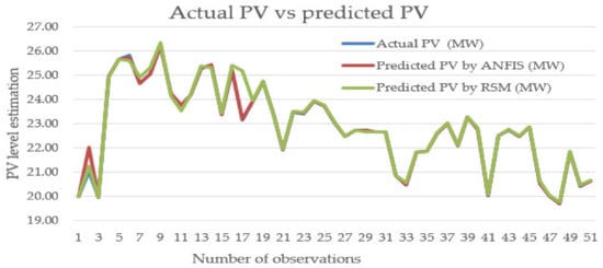
Figure 20.
The comparison of actual and predicted solar PV generation model outcomes.
4.3. Comparison of the Results with the Cases Introduced by Other Works
Naderloo (2020) [34] developed a neural network and RSM methods to predict solar radiation and found out that RSM was superior to the ANFIS model in terms of performance, speed, and simplicity. The correlation coefficients and mean square errors of each method were considered for comparison of the ANFIS (0.993 and 0.0005), ANN (0.996 and 0.00029), and RSM (0.996 and 0.00027). Benmouiza et al. (2019) [35] analyzed the performance of the ANFIS model and found out that RMSE is 102.57 W/m2 for 32 fuzzy rules and 129.13 for 243 fuzzy rules models, and the correlation coefficients were found to be 0.923 and 0.905 for these models, respectively. Mohammadi et al. (2016) [36] developed an ANFIS model for solar radiation based on RMSE during training and testing phases with 1, 2 and 3 fuzzy input parameters. They found that when the number of inputs is increased, the RMSE decreases, and the prediction accuracy enhances. Similarly, in our study, three ANFIS models were developed including five, nine and eleven fuzzy rules based on the sub clustering algorithm. The RMSE of ANFIS model with nine rules gave the best results with minimum error of solar PV generation. The results are presented in Table 3 for comparison. The RMSE was found to be 66.98 for the training process of ANFIS model with nine fuzzy rules, and RMSE was found at 113.52 for ANFIS model with nine rules, and 68.47 for the ANFIS model with eleven fuzzy rules. Aldair et al. (2018) [37] developed ANFIS controllers to determine the stand-alone PV system for which two input variables: the radiation and temperature were considered for the ANFIS model development. The difference between our model and Aldair’s [37] model is that our model was established based on more variables.
Table 3.
The PV power output comparison of ANFIS and RSM models.
The ANFIS and RSM methods developed are highly efficient and effective under different weather conditions especially when the temperature is around 25 °C regardless of the radiation variation. In our study, all PV designs determined for KAU hospital were simulated under the local climate conditions of Jeddah and detailed analysis was carried out and presented in the previous sections of this work. For PV system simulation, the Solar-GIS program [43] and the PVGIS program [44] were used to validate the simulation results obtained from the Solar-GIS program. Figure 8 shows the comparison of monthly electricity generation obtained from both the PV-GIS and the Solar-GIS programs for a 25 MW PV system.
5. Conclusions
This study covers an on-grid PV system design in accordance with a self-consumption model developed for KAU Hospital. The solar PV system was simulated. In the design, the data of Harran university hospital, which produces electrical energy with the solar power plant, were used. The annual average PV electricity (AC) delivered by the total established capacity of the PV system was found to be 1843 kWh/kWp.
- A solar PV system with a capacity of 35 MW and/or more will be sufficient for the KAU hospital and meet the electrical energy demand of the hospital;
- For a PV system of 40 MW capacity, the maximum electricity generation is approximately between 26 and 31 MWh. Hence, the hourly maximum electrical energy requirement of the hospital between 11:00 and 15:00 h can be met by the PV system during all months;
- In all PV designs and simulation tests, the highest electrical energy production during the year was observed in March;
- The self-sufficiency ratio for March was 31% for PV25, 37% for PV30, 43% for PV35, 50% for PV40, 56% for PV45, 62% for PV50, 93% for PV75 and 124% for PV100;
- The self-sufficiency ratio for the yearly period was found as 24% for PV25, 29% for PV30, 34% for PV35, 39% for PV40, 44% for PV45, 48% for PV50, 73% for PV75 and 97% for PV100.
Additionally, the RSM and ANFIS models were developed to analyze the performance of the solar PV panels’ energy generation system depending on uncertain parameter levels. The conclusions regarding the RSM approach showed that a polynomial model is rational for approximation and can be used for defining the relationships efficiently for the entire space of the independent parameters. Hence, Figure 9 showed the normality, and no extreme evidence pointing to possible outliers. Figure 16 examination showed that the parameters’ lines are not parallel. This is the indication that an interaction exists between the factors. Hence, the optimal solar PV generation can be attained, at average module surface temperature, high radiation, wind direction and wind speed level. Changing from low to high module surface temperature and outdoor temperature reduces the solar PV yield. The optimal level of solar PV generation is achieved with average module surface temperature, high radiation, and high wind speed level. High surface temperature is not desired and can be reduced drastically with wind speed.
The conclusion demonstrated that the ANFIS model with nine rules gave the highest performance with the lowest residual. The ANFIS model can produce and predict the solar PV value for the output parameter regarding predetermined input parameters’ intervals. The Gaussian MFs seems appropriate for defining the fuzzy linguistic terms used in fuzzy rules and in the inner loop of the model for fine-tuning the PV generation. Results and findings showed that the ANFIS model can successfully be utilized for the prediction of solar PV module performance.
As a result, meeting the electricity needs of KAU hospital is possible with a suitable capacity of PV system according to its economic resources. The PV systems’ investment is particularly more attractive nowadays with the reducing PV system cost, and improved PV panel technologies (such as bifacial cell, hetero-junction solar cell). A 40 MW capacity PV system is recommended according to the self-consumption of KAU hospital. In addition, the capacity of the PV system for the self-sufficiency model should be 100 MW.
Author Contributions
The individual contribution of the authors was as follows: Conceptualization, O.T., M.A.A. and R.A.; together designed research, provide extensive advice throughout the study reading to research design, research methodology, data collection, and assessment of the results. Funding acquisition, E.H.-V.; writing—review and editing, R.A., O.T., M.A.A. and E.H.-V. All authors have read and agreed to the published version of the manuscript.
Funding
This work was funded by the Deanship of Scientific Research (DSR), King Abdulaziz University, Jeddah, under grant No. (D1441-135-626). The authors, therefore, acknowledge with thanks DSR technical and financial support.
Institutional Review Board Statement
Not applicable.
Informed Consent Statement
Not applicable.
Data Availability Statement
Data are contained within the article.
Acknowledgments
This work was funded by the Deanship of Scientific Research (DSR), King Abdulaziz University, Jeddah, under grant No. (D1441-135-626). The authors, therefore, acknowledge with thanks DSR for technical and financial support. In addition, the authors thank Harran University Presidency and GAPYENEV center for data supply and technical support.
Conflicts of Interest
The authors declare that they have no competing interests.
References
- Taylan, O.; Alamoudi, R.; Kabli, M.; AlJifri, A.; Ramzi, F.; Herrera-Viedma, E. Assessment of Energy Systems Using Extended Fuzzy AHP. Fuzzy VIKOR. and TOPSIS Approaches to Manage Non-Cooperative Opinions. Sustainability 2020, 12, 2745. [Google Scholar] [CrossRef] [Green Version]
- Bersano, A.; Segantin, S.; Falcone, N.; Panella, B.; Testoni, R. Evaluation of a potential reintroduction of nuclear energy in Italy to accelerate the energy transition. Electr. J. 2020, 33, 106813. [Google Scholar] [CrossRef]
- Khan, M.M.A.; Asif, M.; Stach, E. Rooftop PV Potential in the Residential Sector of the Kingdom of Saudi Arabia. Buildings 2017, 7, 46. [Google Scholar] [CrossRef]
- Almasoud, A.H.; Gandayh, H.M. Future of solar energy in Saudi Arabia. J. King Saud Univ. Eng. Sci. 2015, 27, 153–157. [Google Scholar] [CrossRef] [Green Version]
- Belloumi, M.; Alshehry, A. Sustainable Energy Development in Saudi Arabia. Sustainability 2015, 7, 5153–5170. [Google Scholar] [CrossRef] [Green Version]
- Alnaser, W.E.; Alnaser, N.W. The status of renewable energy in the GCC countries. Renew. Sustain. Energy Rev. 2011, 15, 3074–3098. [Google Scholar] [CrossRef]
- Yıldırım, E.; Aktacir, M.A. Optimization of PV System and Technology in View of a Load Profile: Case of Public Building in Turkey. Therm. Sci. 2019, 23, 3567–3577. [Google Scholar] [CrossRef] [Green Version]
- Martin, A.G.; Yoshihiro, H.; Wilhelm, W.; Ewan, D.D.; Dean, H.L.; Jochen, H.; Anita, W.H.H.B. Solar cell efficiency tables (version 50). Prog. Photovolt. Res. Appl. 2017, 25, 668–676. [Google Scholar]
- Mehrabankhomartash, M.; Rayati, M.; Sheikhi, A.; Ranjbar, A.M. Practical battery size optimization of a PV system by considering individual customer damage function. Renew. Sustain. Energy Rev. 2017, 67, 36–50. [Google Scholar] [CrossRef]
- Kaldellis, J.K.; Kapsali, M.; Kavadias, K.A. Temperature and wind speed impact on the efficiency of PV installations. Experience obtained from outdoor measurements in Greece. Renew. Energy 2014, 66, 612–624. [Google Scholar] [CrossRef]
- Bai, A.; Popp, J.; Balogh, P.; Gabnai, Z.; Pályi, B.; Farkas, I.; Pintér, G.; Zsiborács, H. Technical and economic effects of cooling of monocrystalline photovoltaic modules under Hungarian conditions. Renew. Sustain. Energy Rev. 2016, 60, 1086–1099. [Google Scholar] [CrossRef] [Green Version]
- Grubisic-Cabo, F.; Sandro, N.; Giuseppe, T. Photovoltaic panels: A review of the cooling techniques. Trans. FAMENA 2016, 40, 63–74. [Google Scholar]
- Makrides, G.; Zinsser, B.; Norton, M.; Georghiou, G.E. Performance of Photovoltaics Under Actual Operating Conditions. In Third Generation Photovoltaics; Springer: Berlin/Heidelberg, Germany, 2012; ISBN 978-953-51-0304-2. [Google Scholar]
- Lee, S.; Lee, H.; Yoon, B. Modeling and analyzing technology innovation in the energy sector: Patent-based HMM approach. Comput. Ind. Eng. 2012, 63, 564–577. [Google Scholar] [CrossRef]
- Fan, Y. Energy Management and Economics. Comput. Ind. Eng. 2012, 63, 539–728. [Google Scholar] [CrossRef]
- Tian, G.; Liu, Y.; Ke, H.; Chu, J. Energy evaluation method and its optimization models for process planning with stochastic characteristics: A case study in disassembly decision-making. Comput. Ind. Eng. 2012, 63, 553–563. [Google Scholar] [CrossRef]
- Akpolat, A.N.; Dursun, E.; Kuzucuoğlu, A.E.; Yang, Y.; Blaabjerg, F.; Baba, A.F. Performance Analysis of a Grid-Connected Rooftop Solar Photovoltaic System. Electronics 2019, 8, 905. [Google Scholar] [CrossRef] [Green Version]
- Muteri, V.; Cellura, M.; Curto, D.; Franzitta, V.; Longo, S.; Mistretta, M.; Parisi, M.L. Review on Life Cycle Assessment of Solar Photovoltaic Panels. Energies 2020, 13, 252. [Google Scholar] [CrossRef] [Green Version]
- Pradhan, A.K.; Kar, S.K.; Mohanty, M.K. Grid Renewable Hybrid Power Generation System for a Public Health Centre in Rural Village. Int. J. Renew. Energy Res. 2016, 6, 282–288. [Google Scholar]
- Almarshoud, A. Performance of solar resources in Saudi Arabia. Renew. Sustain. Energy Rev. 2016, 66, 694–701. [Google Scholar] [CrossRef]
- Mittal, M.; Bora, B.; Saxena, S.; Gaur, A.M. Performance prediction of PV module using electrical equivalent model and artificial neural network. Sol. Energy 2018, 176, 104–117. [Google Scholar] [CrossRef]
- Yahya-Khotbehsara, A.; Shahhoseini, A. A fast modeling of the double-diode model for PV modules using combined analytical and numerical approach. Sol. Energy 2018, 162, 403–409. [Google Scholar] [CrossRef]
- Goverde, H.; Goossens, D.; Govaerts, J.; Catthoor, F.; Baert, K.; Poortmans, J.; Driesen, J. Spatial and temporal analysis of wind effects on PV modules: Consequences for electrical power evaluation. Sol. Energy 2017, 147, 292–299. [Google Scholar] [CrossRef]
- Goossens, D.; Goverde, H.; Catthoor, F. Effect of wind on temperature patterns, electrical characteristics, and performance of building-integrated and building-applied inclined photovoltaic modules. Sol. Energy 2018, 170, 64–75. [Google Scholar] [CrossRef]
- Curto, D.; Favuzza, S.; Franzitta, V.; Musca, R.; Navarro, M.A.N.; Zizz, G. Evaluation of the optimal renewable electricity mix for Lampedusa island: The adoption of a technical and economical methodology. J. Clean. Prod. 2020, 263, 121404. [Google Scholar] [CrossRef]
- Awan, A.B.; Zubair, M.; Praveen, R.P.; Abokhalil, A.G. Solar Energy Resource Analysis and Evaluation of Photovoltaic System Performance in Various Regions of Saudi Arabia. Sustainability 2018, 10, 1129. [Google Scholar] [CrossRef] [Green Version]
- Rani, P.; Mishra, A.R.; Pardasani, K.R.; Mardani, A.; Liao, H.; Streimikienef, D. A novel VIKOR approach based on entropy and divergence measures of Pythagorean fuzzy sets to evaluate renewable energy technologies in India. J. Clean. Prod. 2019, 238, 117936. [Google Scholar] [CrossRef]
- Daus, Y.V.; Yudaev, I.V.; Stepanchuk, G.V. Reducing the Costs of Paying for Consumed Electric Energy by Utilizing Solar Energy. Appl. Sol. Energy 2018, 54, 139–143. [Google Scholar] [CrossRef]
- Yoomak, Y.; Patcharoen, T.; Ngaopitakkul, A. Performance and Economic Evaluation of Solar Rooftop Systems in Different Regions of Thailand. Sustainability 2019, 11, 6647. [Google Scholar] [CrossRef] [Green Version]
- Kassem, Y.; Camur, H.; Alhuoti, S.M.A. Solar Energy Technology for Northern Cyprus: Assessment, Statistical Analysis, and Feasibility Study. Energies 2020, 13, 940. [Google Scholar] [CrossRef] [Green Version]
- Ascencio-Vásquez, J.; Brecl, K.; Topič, M. Methodology of Köppen-Geiger-Photovoltaic climate classification and implications to worldwide mapping of PV system performance. Sol. Energy 2019, 191, 672–685. [Google Scholar] [CrossRef]
- Zell, E.; Gasim, S.; Wilcox, S.; Katamoura, S.; Stoffel, T.; Shibli, H.; Engel-Cox, J.; Al Subie, M. Assessment of solar radiation resources in Saudi Arabia. Sol. Energy 2015, 119, 422–438. [Google Scholar] [CrossRef] [Green Version]
- Roy, P.; Sinha, N.K.; Tiwari, S.; Khare, A. A review on perovskite solar cells: Evolution of architecture, fabrication techniques, commercialization issues and status. Sol. Energy 2020, 198, 665–688. [Google Scholar] [CrossRef]
- Naderloo, L. Prediction of solar radiation on the horizon using NN methods, ANFIS and RSM (Case study-Iran). J. Earth Syst. Sci. 2020, 129, 148. [Google Scholar]
- Benmouiza, K.; Cheknane, A. Clustered ANFIS network using fuzzy c-means, subtractive clustering, and grid partitioning for hourly solar radiation forecasting. Theor. Appl. Climatol. 2019, 137, 31–43. [Google Scholar] [CrossRef]
- Mohammadi, K.; Shamshirband, S.; Kamsin, A.; Lai, P.C.; Mansor, Z. Identifying the most significant input parameters for predicting global solar radiation using an ANFIS selection procedure. Renew. Sustain. Energy Rev. 2016, 63, 423–434. [Google Scholar] [CrossRef]
- Aldair, A.A.; Obed, A.A.; Halihal, A.F. Design and implementation of ANFIS-reference model controller based MPPT using FPGA for photovoltaic system. Renew. Sustain. Energy Rev. 2018, 82, 2202–2217. [Google Scholar] [CrossRef]
- Khosravi, A.; Malekan, M.; Pabon, J.J.G.; Zhao, X.; Assad, M.E.H. Design parameter modelling of solar power tower system using adaptive neuro-fuzzy inference system optimized with a combination of genetic algorithm and teaching learning-based optimization algorithm. J. Clean. Prod. 2020, 244, 118904. [Google Scholar] [CrossRef]
- Solar-GIS. Available online: https://globalsolaratlas.info/map (accessed on 30 May 2020).
- PVGIS. Available online: https://ec.europa.eu/jrc/en/pvgis (accessed on 30 May 2020).
- Colak, N.S.; Sahin, E.; Dertli, E.; Yilmaz, M.T.; Taylan, O. Response surface methodology as optimization strategy for asymmetric bioreduction of acetophenone using whole cell of Lactobacillus senmaizukei. Prep. Biochem. Biotechnol. 2019, 49, 884–890. [Google Scholar] [CrossRef] [PubMed]
- Dirnberger, D.; Kräling, U. Uncertainty in PV Module Measurement—Part I: Calibration of Crystalline and Thin-Film Modules. IEEE J. Photovolt. 2013, 3, 1016–1026. [Google Scholar] [CrossRef]
- Taylan, O.; Darrab, I.A. Fuzzy control charts for process quality improvement and product assessment in tip shear carpet industry. J. Manuf. Technol. Manag. 2012, 23, 402–420. [Google Scholar] [CrossRef]
- Taylan, O.; Taşkın, H. Fuzzy Modelling af A Production System. J. Nav. Sci. Eng. 2003, 1, 1–13. [Google Scholar]
- Taylan, O.; Karagozoglu, B. An Adaptive Neuro-Fuzzy Model for Prediction of Student’s Academic Performance. Comput. Ind. Eng. 2009, 57, 732–741. [Google Scholar] [CrossRef]
- Taylan, O. Neural and fuzzy model performance evaluation of a dynamic production system. Int. J. Prod. Res. 2006, 44, 1093–1105. [Google Scholar] [CrossRef]
- Taylan, O.; Darrab, I.A. Determining optimal quality distribution of latex weight using adaptive neuro-fuzzy modeling and control systems. Comput. Ind. Eng. 2011, 61, 686–696. [Google Scholar] [CrossRef]
- Al-Ghamdi, K.; Taylan, O. A comparative study on modelling material removal rate by ANFIS and polynomial methods in electrical discharge machining process. Comput. Ind. Eng. 2015, 79, 27–41. [Google Scholar] [CrossRef]


Publisher’s Note: MDPI stays neutral with regard to jurisdictional claims in published maps and institutional affiliations. |
© 2021 by the authors. Licensee MDPI, Basel, Switzerland. This article is an open access article distributed under the terms and conditions of the Creative Commons Attribution (CC BY) license (https://creativecommons.org/licenses/by/4.0/).