A Note on the Boundedness of Doob Maximal Operators on a Filtered Measure Space

Abstract

Let M be the Doob maximal operator on a filtered measure space and let v be an $A_p$ weight with $1<p<+\infty$. We try proving that ${\parallel Mf\parallel }_{L^p\left(v\right)}\le p^{\prime }{\left[v\right]}_{A_p}^{\frac{1}{p-1}}{\parallel f\parallel }_{L^p\left(v\right)},$ where $1/p+1/p^{\prime }=1.$ Although we do not find an approach which gives the constant $p^{\prime },$ we obtain that ${\parallel Mf\parallel }_{L^p\left(v\right)}\le p^{\frac{1}{p-1}}{p}^{\prime }{\left[v\right]}_{A_p}^{\frac{1}{p-1}}{\parallel f\parallel }_{L^p\left(v\right)},$ with $\underset{p\to +\infty }{lim}{p}^{\frac{1}{p-1}}=1.$

1. Introduction

Let M be the Doob maximal operator on a filtered measure space. For $1<p<+\infty ,$ it is well known (see, e.g., [1]) that

$${\parallel Mf\parallel }_{L^p}\le p^{\prime }{\parallel f\parallel }_{L^p},$$

(1)

where $1/p+1/p^{\prime }=1$ and $p^{\prime }$ is the best constant. Let v be an $A_p$ weight with $1<p<+\infty .$ Tanaka and Terasawa [2] proved that

$${\parallel Mf\parallel }_{L^p\left(v\right)}\le C{\left[v\right]}_{A_p}^{\frac{1}{p-1}}{\parallel f\parallel }_{L^p\left(v\right)},$$

(2)

where C is independent of $v.$

For a Euclidean space with a dyadic filtration, the dyadic maximal operator is the above Doob maximal operator. For the dyadic maximal operator, the constant $1/(p-1)$ is the optimal power on ${\left[v\right]}_{A_p}$(see, e.g., [3,4]). It follows that the constant $1/(p-1)$ is also the optimal power on ${\left[v\right]}_{A_p}$ for the Doob maximal operator $M.$

In this note, we estimate the constant C in (2). Substituting $v=1$ into (2), we get (1). Thus, we conjecture that the constant C equals $p^{\prime }$ in (2). However, we do not find an approach which gives the constant $C=p^{\prime }.$ Our results are as follows.

Theorem 1. 

Let v be a weight and $1<p<\infty .$ We have the inequality

$${\parallel Mf\parallel }_{L^p\left(v\right)}\le C{\parallel f\parallel }_{L^p\left(v\right)}$$

(3)

if and only if $v\in A_p$. Moreover, if we denote the smallest constant in (3) by $\parallel M\parallel$, we have

$${\left[v\right]}_{A_p}\le {\parallel M\parallel }^p$$

(4)

and

$$\parallel M\parallel \le p^{\frac{1}{p-1}}{p}^{\prime }{\left[v\right]}_{A_p}^{\frac{1}{p-1}}.$$

(5)

Remark 1. 

The content of Theorem 1 is (5). In order to prove (5), we use different approaches as follows:

1 

Motivated by the proof of [4] (Theorem B), we get $C=p^{\frac{1}{p-1}}{p}^{\prime }.$

2 

Using the construction of principal sets [2] and the conditional sparsity [5], we have $C=a^2{\eta }^{(p^{\prime }-1)}{p}^{\prime },$ where $a,\eta$ are the constants in the construction of principal sets (Appendix A).

3 

Long [1] [Theorem 6.6.3] qualitatively evaluated $\parallel M\parallel$. Modifying Long’s proof, we have $C=p^{\frac{1}{p-1}}{p}^{\prime }$ which is the same as 1.

Approaches 1 and 3 both use the boundedness of the Doob maximal operator twice and give the same estimation $C=p^{\frac{1}{p-1}}{p}^{\prime }.$ Approach 2 depends on the conditional sparsity and the boundedness of the Doob maximal operator. Letting $\sigma =v^{\frac{1}{p-1}}$ and $f=h\sigma ,$ we can rewrite (3) as

$${\parallel M\left(h\sigma \right)\parallel }_{L^p\left(v\right)}\le C{\parallel h\sigma \parallel }_{L^p\left(\sigma \right).}$$

Cao and Xue [6] (see also the references therein) used the atomic decomposition to study weighted theory on the Euclidean space, but we do not know whether it is possible on the filtered measure space.

This paper is organized as follows. Section 2 consists of the preliminaries for this paper. In Section 3, we give the proof of Theorem 1, and in Section 4 we compare $p^{\frac{1}{p-1}}$ with $a^2{\eta }^{(p^{\prime }-1)}$. In order to keep track of the constants in our paper, we modify the construction of principal sets in Appendix A.

2. Preliminaries

The filtered measure space was discussed in [2,7], which is abstract and contains several kinds of spaces. For example, a doubling metric space with systems of dyadic cubes was introduced by Hytönen and Kairema [8]. In order to develop discrete martingale theory, a probability space endowed with a family of $\sigma$-algebra was considered by Long [1]. In addition, a Euclidean space with several adjacent systems of dyadic cubes was mentioned by Hytönen [9]. Because the filtered measure space is abstract, it is possible to study these spaces together ([10,11,12]). As is well known, Lacey, Petermichl and Reguera [13] studied the shift operators, which are related to the martingale theory on a filtered measure space. When Hytönen [9] solved the conjecture of $A_2,$ those operators became very useful.

2.1. Filtered Measure Space

Let $(\mathrm{\Omega },\mathcal{F},\mu )$ be a measure space and let ${\mathcal{F}}^0=\bigcup \{E:E\in \mathcal{F},\mu \left(E\right)<+\infty \}$. As for $\sigma$-finite, we mean that $\mathrm{\Omega }$ is a union of ${\left(E_i\right)}_{i\in \mathbb{Z}}\subset {\mathcal{F}}^0.$ We only consider $\sigma$-finite measure space $(\mathrm{\Omega },\mathcal{F},\mu )$ in this paper. Let $\mathcal{B}$ be a sub-family of ${\mathcal{F}}^0$ and let $f:\mathrm{\Omega }\to \mathbb{R}$ be measurable on $(\mathrm{\Omega },\mathcal{F},\mu )$. If for all $B\in \mathcal{B}$, we have ${\int }_B\left|f\right|d\mu <+\infty ,$ then we say that f is $\mathcal{B}$-integrable. The family of the above functions is denoted by $L_{\mathcal{B}}^1(\mathcal{F},\mu ).$

Let $\mathcal{B}\subset \mathcal{F}$ be a sub-$\sigma$-algebra and let $f\in L_{{\mathcal{B}}^0}^1(\mathcal{F},\mu )$. Because of the $\sigma$-finiteness of $(\mathrm{\Omega },\mathcal{B},\mu )$ and Radon–Nikodým’s theorem, there is a unique function denoted by $\mathbb{E}\left(f\right|\mathcal{B})\in L_{{\mathcal{B}}^0}^1(\mathcal{B},\mu )$ or ${\mathbb{E}}_{\mathcal{B}}\left(f\right)\in L_{{\mathcal{B}}^0}^1(\mathcal{B},\mu )$ such that

$${\int }_{B}fd\mu ={\int }_B{\mathbb{E}}_{\mathcal{B}}\left(f\right)d\mu ,\forall B\in {\mathcal{B}}^0.$$

Letting $(\mathrm{\Omega },\mathcal{F},\mu )$ with a family ${\left({\mathcal{F}}_i\right)}_{i\in \mathbb{Z}}$ of sub-$\sigma$-algebras satisfying that ${\left({\mathcal{F}}_i\right)}_{i\in \mathbb{Z}}$ is increasing, we say that $\mathcal{F}$ has a filtration ${\left({\mathcal{F}}_i\right)}_{i\in \mathbb{Z}}$. Then, a quadruplet $(\mathrm{\Omega },\mathcal{F},\mu ;{\left({\mathcal{F}}_i\right)}_{i\in \mathbb{Z}})$ is said to be a filtered measure space. It is clear that $L_{{\mathcal{F}}_i^0}^1(\mathcal{F},\mu )\supset L_{{\mathcal{F}}_j^0}^1(\mathcal{F},\mu )$ with $i<j.$ Let $\mathcal{L}:={\displaystyle \bigcap _{i\in \mathbb{Z}}}{L}_{{\mathcal{F}}_i^0}^1(\mathcal{F},\mu )$ and $f\in \mathcal{L},$ then ${\left({\mathbb{E}}_i\left(f\right)\right)}_{i\in \mathbb{Z}}$ is a martingale, where ${\mathbb{E}}_i\left(f\right)$ means $\mathbb{E}\left(f\right|{\mathcal{F}}_i).$ The reason is that ${\mathbb{E}}_i\left(f\right)={\mathbb{E}}_i\left({\mathbb{E}}_{i+1}\left(f\right)\right),$ $i\in \mathbb{Z}.$

2.2. Stopping Times

Let $(\mathrm{\Omega },\mathcal{F},\mu ;{\left({\mathcal{F}}_i\right)}_{i\in \mathbb{Z}})$ be a $\sigma$-finite filtered measure space and let $\tau :\mathrm{\Omega }\to \{-\infty \}\cup \mathbb{Z}\cup \{+\infty \}$. If for any $i\in \mathbb{Z},$ we have $\{\tau =i\}\in {\mathcal{F}}_i,$ then $\tau$ is said to be a stopping time. We denote the family of all stopping times by $\mathcal{T}.$ For $i\in \mathbb{Z},$ we denote ${\mathcal{T}}_i:=\{\tau \in \mathcal{T}:\tau \ge i\}.$

2.3. Operators and Weights

Let $f\in \mathcal{L}.$ The Doob maximal operator is defined by

$$Mf=\underset{i\in \mathbb{Z}}{sup}\left|{\mathbb{E}}_i\left(f\right)\right|.$$

For $i\in \mathbb{Z},$ we define the tailed Doob maximal operator by

$${{}^{*}M}_{i}f=\underset{j\ge i}{sup}\left|{\mathbb{E}}_j\left(f\right)\right|.$$

For $\omega \in \mathcal{L}$ with $\omega \ge 0,$ we say that $\omega$ is a weight. The set of all weights is denoted by ${\mathcal{L}}^{+}.$ Let $B\in \mathcal{F},$ $\omega \in {\mathcal{L}}^{+}.$ Then ${\int }_{\mathrm{\Omega }}{\chi }_{B}d\mu$ and ${\int }_{\mathrm{\Omega }}{\chi }_B\omega d\mu$ are denoted by $\left|B\right|$ and ${\left|B\right|}_{\omega },$ respectively. Now we give the definition of $A_p$ weights.

Definition 1. 

Let $1<p<\infty$ and let ω be a weight. We say that the weight ω is an $A_p$ weight, if there exists a positive constant C such that

$$\underset{j\in \mathbb{Z}}{sup}{\mathbb{E}}_j\left(\omega \right){\mathbb{E}}_j{({\omega }^{1-p^{\prime }})}^{\frac{p}{p^{\prime }}}\le C,$$

(6)

where $\frac{1}{p}+\frac{1}{p^{\prime }}=1.$ We denote the smallest constant C in (6) by ${\left[\omega \right]}_{A_p}$.

3. Approaches of Theorem 1

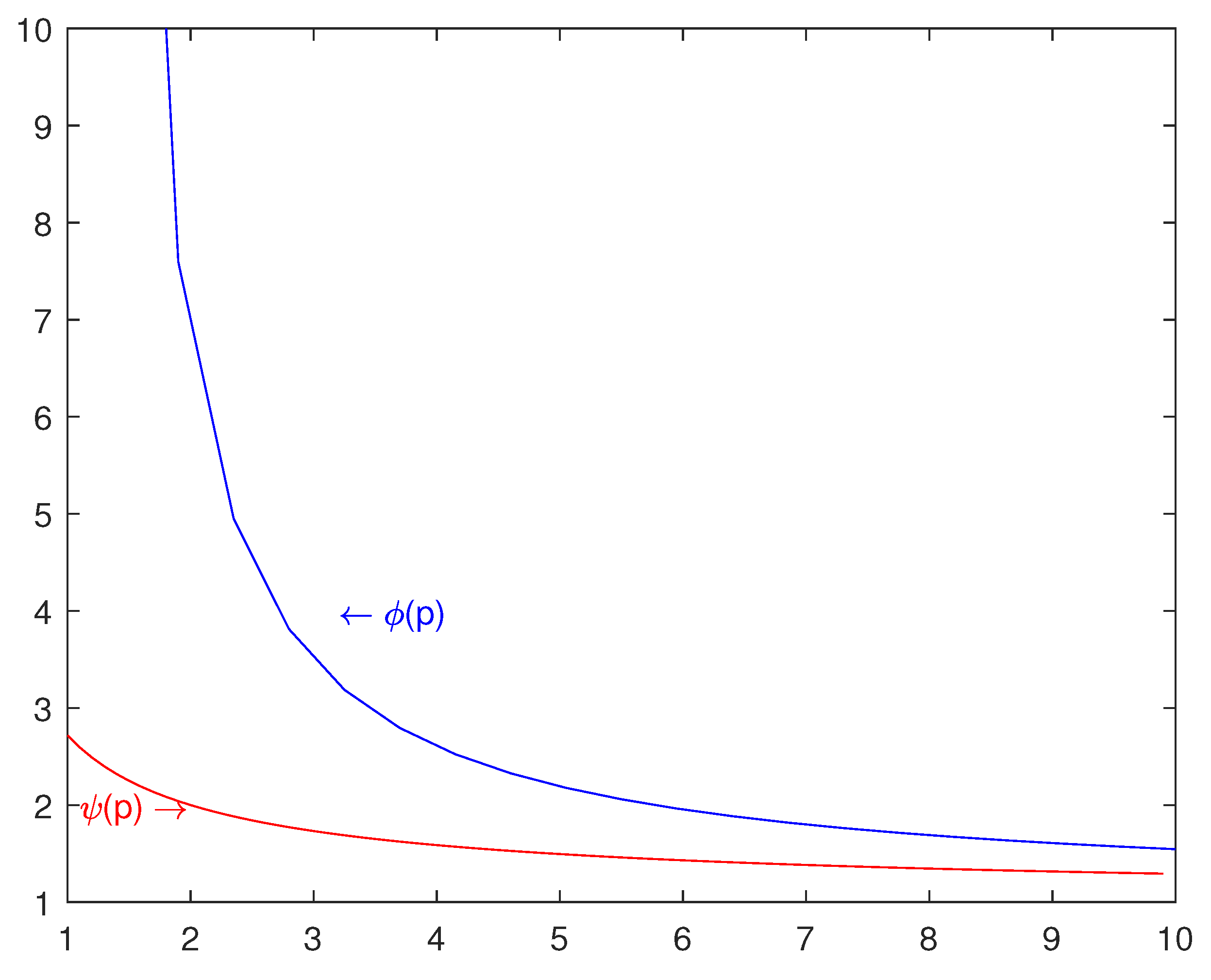
Proof of Theorem 1. 

We prove that (3) implies (4). For $i\in \mathbb{Z}$ and $B\in {\mathcal{F}}_i^0,$ we let $f={\chi }_B.$

Then

$${\mathbb{E}}_i(v^{-\frac{1}{p-1}}){\chi }_B\le M\left(f\sigma \right){\chi }_B,$$

where $\sigma =v^{\frac{1}{p-1}}.$ It follows from (3) that

$$\begin{array}{c}\hfill {\left({\int }_B{\mathbb{E}}_i{(v^{-\frac{1}{p-1}})}^{p}vd\mu \right)}^{\frac{1}{p}}\le \parallel M\parallel {\left({\int }_{\mathrm{\Omega }}{v}^{-\frac{1}{p-1}}{\chi }_{B}d\mu \right)}^{\frac{1}{p}}.\end{array}$$

Thus

$$\begin{array}{c}\hfill {\mathbb{E}}_i{(v^{-\frac{1}{p-1}})}^p{\mathbb{E}}_i\left(v\right)\le {\parallel M\parallel }^p{\mathbb{E}}_i(v^{-\frac{1}{p-1}}),\end{array}$$

which shows that

$${\left[v\right]}_{A_p}\le {\parallel M\parallel }^p.$$

In order to prove (5), we provide the three approaches which we mentioned in Remark 1.

Approach 1. It is clear that

$$\begin{array}{ccc}\hfill {\mathbb{E}}_n\left(f\right)& =& ({\mathbb{E}}_n\left(v\right){\mathbb{E}}_n{\left(\sigma \right)}^{p-1}\frac{1}{{\mathbb{E}}_n\left(v\right)}(\frac{1}{{\mathbb{E}}_n\left(\sigma \right)}{\mathbb{E}}_n\left(f\right){)}^{p-1}{)}^{\frac{1}{p-1}}\hfill \\ & =& {\left({\mathbb{E}}_n\left(v\right){\mathbb{E}}_n{\left(\sigma \right)}^{p-1}\right)}^{\frac{1}{p-1}}{\left(\frac{1}{{\mathbb{E}}_n\left(v\right)}(\frac{1}{{\mathbb{E}}_n\left(\sigma \right)}{\mathbb{E}}_n\left(f\right){)}^{p-1}\right)}^{\frac{1}{p-1}}\hfill \\ & \le & {\left[v\right]}_{A_p}^{\frac{1}{p-1}}{M}^v({v^{-1}{M}^{\sigma }{\left(f{\sigma }^{-1}\right)}^{p-1}}^{\frac{1}{p-1}}).\hfill \end{array}$$

Then, we have

$$\begin{array}{c}\hfill M\left(f\right)\le {\left[v\right]}_{A_p}^{\frac{1}{p-1}}{M}^v({v^{-1}{M}^{\sigma }{\left(f{\sigma }^{-1}\right)}^{p-1}}^{\frac{1}{p-1}}).\end{array}$$

Using the boundedness of Doob maximal operators $M^v$ and $M^{\sigma },$ we obtain

$$\begin{array}{ccc}\hfill {\parallel M\left(f\right)\parallel }_{L^p\left(v\right)}& \le & {\left[v\right]}_{A_p}^{\frac{1}{p-1}}{\parallel M^v{\left(v^{-1}{M}^{\sigma }{\left(f{\sigma }^{-1}\right)}^{p-1}\right)}^{\frac{1}{p-1}}\parallel }_{L^p\left(v\right)}\hfill \\ & =& {\left[v\right]}_{A_p}^{\frac{1}{p-1}}{\parallel M^v\left(v^{-1}{M}^{\sigma }{\left(f{\sigma }^{-1}\right)}^{p-1}\right)\parallel }_{L^{p^{\prime }}\left(v\right)}^{\frac{1}{p-1}}\hfill \\ & \le & p^{\frac{1}{p-1}}{\left[v\right]}_{A_p}^{\frac{1}{p-1}}{\parallel M^{\sigma }\left(f{\sigma }^{-1}\right)\parallel }_{L^p\left(\sigma \right)}\hfill \\ & \le & p^{\frac{1}{p-1}}{p}^{\prime }{\left[v\right]}_{A_p}^{\frac{1}{p-1}}{\parallel f\parallel }_{L^p\left(v\right)}.\hfill \end{array}$$

Approach 2. For $i\in \mathbb{Z},$ $k\in \mathbb{Z}$ and ${\mathrm{\Omega }}_0\in {\mathcal{F}}_i^0,$ we denote

$$P_0=\{a^{k-1}<\mathbb{E}\left(f\sigma \right|{\mathcal{F}}_i)\le a^k\}\cap {\mathrm{\Omega }}_0.$$

We claim that

$${\left({\int }_{P_0}{}^{*}{M}_i{\left(f\sigma {\chi }_{P_0}\right)}^{p}vd\mu \right)}^{\frac{1}{p}}\le a^2{\eta }^{(p^{\prime }-1)}{p}^{\prime }{\left[v\right]}_{A_p}^{\frac{p^{\prime }}{p}}{\left({\int }_{P_0}{f}^p\sigma d\mu \right)}^{\frac{1}{p}},$$

(7)

where $a,\eta$ are the constants in the construction of principal sets (Appendix A). To see this, we denote $h=f\sigma {\chi }_{P_0}.$ For the above $i,$ $P_0$ and $h,$ we construct principal sets. Then, Lemma A1 shows that

$${\int }_{P_0}{}^{*}{M}_i{\left(f\sigma \right)}^{p}vd\mu \le a^{2p}\sum _{P\in \mathcal{P}}{\int }_{E\left(P\right)}{a}^{p({\mathcal{K}}_2\left(P\right)-1)}vd\mu .$$

(8)

To estimate ${\left|E\left(P\right)\right|}_v.$ For the sake of simplicity, we denote $E_{{\mathcal{F}}_{{\mathcal{K}}_1\left(P\right)}}(·)$ by $E_P(·)$ without confusion. We now estimate ${\left|E\left(P\right)\right|}_v$ as follows:

$$\begin{array}{ccc}\hfill {\left|E\left(P\right)\right|}_v& \le & {\left|P\right|}_v={\int }_P{\mathbb{E}}_P\left(v\right)d\mu \hfill \\ & =& {\int }_P{\mathbb{E}}_P{\left(v\right)}^{p^{\prime }}{\mathbb{E}}_P{\left(v\right)}^{1-p^{\prime }}{\mathbb{E}}_P{\left(\sigma \right)}^p{\mathbb{E}}_P{\left(\sigma \right)}^{-p}d\mu \hfill \\ & =& {\int }_P{\mathbb{E}}_P{\left(v\right)}^{p^{\prime }}{\mathbb{E}}_P{\left(\sigma \right)}^p{\mathbb{E}}_P{\left(v\right)}^{1-p^{\prime }}{\mathbb{E}}_P{\left(\sigma \right)}^{-p}d\mu .\hfill \end{array}$$

In the view of the definition of $A_p$ and the construction of $\mathcal{P},$ we have

$$\begin{array}{ccc}\hfill {\left|E\left(P\right)\right|}_v& \le & {\left[v\right]}_{A_p}^{p^{\prime }}{\int }_P{\mathbb{E}}_P{\left(v\right)}^{1-p^{\prime }}{\mathbb{E}}_P{\left(\sigma \right)}^{-p}d\mu \hfill \\ & \le & {\eta }^{p(p^{\prime }-1)}{\left[v\right]}_{A_p}^{p^{\prime }}{\int }_P{\mathbb{E}}_P{\left(v\right)}^{1-p^{\prime }}{\mathbb{E}}_P{\left(\sigma \right)}^{-p}{\mathbb{E}}_P{\left({\chi }_{E\left(P\right)}\right)}^{p(p^{\prime }-1)}d\mu \hfill \\ & =& {\eta }^{p(p^{\prime }-1)}{\left[v\right]}_{A_p}^{p^{\prime }}{\int }_P{\mathbb{E}}_P{\left(v\right)}^{1-p^{\prime }}{\mathbb{E}}_P{\left(\sigma \right)}^{-p}{\mathbb{E}}_P{({\chi }_{E\left(P\right)}{v}^{\frac{1}{p}}{\sigma }^{\frac{1}{p^{\prime }}})}^{p(p^{\prime }-1)}d\mu .\hfill \end{array}$$

Noting that the conditional expectation satisfies Hölder’s inequality, we have

$$\begin{array}{ccc}\hfill {\left|E\left(P\right)\right|}_v& \le & {\eta }^{p(p^{\prime }-1)}{\left[v\right]}_{A_p}^{p^{\prime }}{\int }_P{\mathbb{E}}_P{\left(v\right)}^{1-p^{\prime }}{\mathbb{E}}_P{\left(\sigma \right)}^{-p}\hfill \\ & & \times {\mathbb{E}}_P{\left(v{\chi }_{E\left(P\right)}\right)}^{p^{\prime }-1}{\mathbb{E}}_P\left(\sigma {\chi }_{E\left(P\right)}\right)d\mu \hfill \\ & \le & {\eta }^{p(p^{\prime }-1)}{\left[v\right]}_{A_p}^{p^{\prime }}{\int }_P{\mathbb{E}}_P{\left(\sigma \right)}^{-p}{\mathbb{E}}_P\left(\sigma {\chi }_{E\left(P\right)}\right)d\mu .\hfill \end{array}$$

As $E\left(P\right)$ is a subset of P and $a^{{\mathcal{K}}_2\left(P\right)-1}{\chi }_P\le {\mathbb{E}}_P\left(h\right){\chi }_P,$ we obtain that

$$\begin{array}{ccc}\hfill {\int }_{E\left(P\right)}{a}^{p({\mathcal{K}}_2\left(P\right)-1)}vd\mu & \le & {\eta }^{p(p^{\prime }-1)}{\left[v\right]}_{A_p}^{p^{\prime }}{\int }_P{\mathbb{E}}_P{\left(f\sigma \right)}^p{\mathbb{E}}_P{\left(\sigma \right)}^{-p}{\mathbb{E}}_P\left({\chi }_{E\left(P\right)}\sigma \right)d\mu \hfill \\ & =& {\eta }^{p(p^{\prime }-1)}{\left[v\right]}_{A_p}^{p^{\prime }}{\int }_P{\mathbb{E}}_P^{\sigma }{\left(f\right)}^p{\mathbb{E}}_P\left({\chi }_{E\left(P\right)}\sigma \right)d\mu ,\hfill \end{array}$$

where we have used ${\mathbb{E}}_P\left(f\sigma \right)={\mathbb{E}}_P^{\sigma }\left(f\right){\mathbb{E}}_P\left(\sigma \right).$ Then,

$$\begin{array}{ccc}\hfill {\int }_{E\left(P\right)}{a}^{p({\mathcal{K}}_2\left(P\right)-1)}vd\mu & \le & {\eta }^{p(p^{\prime }-1)}{\left[v\right]}_{A_p}^{p^{\prime }}{\int }_P{\mathbb{E}}_P^{\sigma }{\left(f\right)}^p{\mathbb{E}}_P\left({\chi }_{E\left(P\right)}\sigma \right)d\mu \hfill \\ & =& {\eta }^{p(p^{\prime }-1)}{\left[v\right]}_{A_p}^{p^{\prime }}{\int }_P{\mathbb{E}}_P^{\sigma }{\left(f\right)}^p{\chi }_{E\left(P\right)}\sigma d\mu \hfill \\ & \le & {\eta }^{p(p^{\prime }-1)}{\left[v\right]}_{A_p}^{p^{\prime }}{\int }_P{M}^{\sigma }{\left(f{\chi }_{P_0}\right)}^p{\chi }_{E\left(P\right)}\sigma d\mu \hfill \\ & =& {\eta }^{p(p^{\prime }-1)}{\left[v\right]}_{A_p}^{p^{\prime }}{\int }_{E\left(P\right)}{M}^{\sigma }{\left(f{\chi }_{P_0}\right)}^p\sigma d\mu .\hfill \end{array}$$

It follows from (8) and the boundedness of Doob maximal operator $M^{\sigma }$ that

$$\begin{array}{ccc}\hfill {\int }_{P_0}{}^{*}{M}_i{\left(f\sigma \right)}^{p}vd\mu & \le & a^{2p}{\eta }^{p(p^{\prime }-1)}{\left[v\right]}_{A_p}^{p^{\prime }}\sum _{P\in \mathcal{P}}{\int }_{E\left(P\right)}{M}^{\sigma }{\left(f{\chi }_{P_0}\right)}^p\sigma d\mu \hfill \\ & \le & a^{2p}{\eta }^{p(p^{\prime }-1)}{\left[v\right]}_{A_p}^{p^{\prime }}\sum _{P\in \mathcal{P}}{\int }_{E\left(P\right)}{M}^{\sigma }{\left(f{\chi }_{P_0}\right)}^p\sigma d\mu \hfill \\ & \le & a^{2p}{\eta }^{p(p^{\prime }-1)}{\left(p^{\prime }\right)}^p{\left[v\right]}_{A_p}^{p^{\prime }}{\int }_{P_0}{f}^p\sigma d\mu ,\hfill \end{array}$$

which implies (7). Furthermore,

$$\begin{array}{ccc}\hfill {\int }_{{\mathrm{\Omega }}_0}{}^{*}{M}_i{\left(f\sigma \right)}^{p}vd\mu & =& \sum _{k\in \mathbb{Z}}{\int }_{\{a^{k-1}<E\left(f\sigma \right|{\mathcal{F}}_i)\le a^k\}\cap {\mathrm{\Omega }}_0}{}^{*}{M}_i{\left(f\sigma \right)}^{p}vd\mu \hfill \\ & \le & a^{2p}{\eta }^{p(p^{\prime }-1)}{\left(p^{\prime }\right)}^p{\left[v\right]}_{A_p}^{p^{\prime }}\sum _{k\in \mathbb{Z}}{\int }_{\{a^{k-1}<E\left(f\sigma \right|{\mathcal{F}}_i)\le a^k\}\cap {\mathrm{\Omega }}_0}{f}^p\sigma d\mu \hfill \\ & \le & a^{2p}{\eta }^{p(p^{\prime }-1)}{\left(p^{\prime }\right)}^p{\left[v\right]}_{A_p}^{p^{\prime }}{\int }_{{\mathrm{\Omega }}_0}{f}^p\sigma d\mu .\hfill \end{array}$$

Noting that $(\mathrm{\Omega },\mathcal{F},\mu )$ is a $\sigma$-finite measure space, we obtain that

$$\begin{array}{ccc}\hfill {({\int }_{\mathrm{\Omega }}{}^{*}{M}_i{\left(f\sigma \right)}^{p}vd\mu )}^{\frac{1}{p}}& \le & a^2{\eta }^{(p^{\prime }-1)}{p}^{\prime }{\left[v\right]}_{A_p}^{\frac{p^{\prime }}{p}}({{\int }_{\mathrm{\Omega }}{f}^p\sigma d\mu }^{\frac{1}{p}}).\hfill \end{array}$$

Because ${}^{*}{M}_i(·)\uparrow M_i(·)$ as $i\downarrow -\infty ,$ then

$$({{\int }_{\mathrm{\Omega }}M{\left(f\sigma \right)}^{p}vd\mu }^{\frac{1}{p}})\le a^2{\eta }^{(p^{\prime }-1)}{p}^{\prime }{\left[v\right]}_{A_p}^{\frac{p^{\prime }}{p}}({{\int }_{\mathrm{\Omega }}{f}^p\sigma d\mu )}^{\frac{1}{p}}.$$

Approach 3. For $f\in L^p\left(vd\mu \right),$ $b>1$ and $k\in \mathbb{Z},$ we define stopping times

$${\tau }_k=inf\{n:|f_n|>b^k\}.$$

Then, we denote

$$A_{k,j}:=\{{\tau }_k<\infty \}\cap \{b^j<\mathbb{E}(\sigma |{\mathcal{F}}_{{\mathcal{F}}_{{\tau }_k}})\le b^{j+1}\}$$

and

$$B_{k,j}:=\{{\tau }_k<\infty ,{\tau }_{k+1}=\infty \}\cap \{b^j<\mathbb{E}(\sigma |{\mathcal{F}}_{{\mathcal{F}}_{{\tau }_k}})\le b^{j+1}\},j\in \mathbb{Z}.$$

It follows that $A_{k,j}\in {\mathcal{F}}_{{\tau }_k},B_{k,j}\subseteq A_{k,j}$. It is clear that ${\left\{B_{k,j}\right\}}_{k,j}$ is a family of disjoint sets and

$$\{b^k<Mf\le b^{k+1}\}=\{{\tau }_k<\infty ,{\tau }_{k+1}=\infty \}=\bigcup _{j\in \mathbb{Z}.}{B}_{k,j},k\in \mathbb{Z}.$$

Following from

$$\mathbb{E}\left(f\right|{\mathcal{F}}_{{\tau }_k})={\mathbb{E}}^{\sigma }\left(f{\sigma }^{-1}\right|{\mathcal{F}}_{{\tau }_k})\mathbb{E}\left(\sigma \right|{\mathcal{F}}_{{\tau }_k}),$$

we have

$$\begin{array}{ccc}\hfill b^{kp}& \le & \underset{A_{k,j}}{\mathrm{ess}\inf }\mathbb{E}{\left(f\right|{\mathcal{F}}_{{\tau }_k})}^p\hfill \\ & \le & \underset{A_{k,j}}{\mathrm{ess}\inf }{\mathbb{E}}^{\sigma }\left(f{\sigma }^{-1}\right|{\mathcal{F}}_{{\tau }_k}{)}^p\underset{A_{k,j}}{\mathrm{ess}\sup }\mathbb{E}{\left(\sigma \right|{\mathcal{F}}_{{\tau }_k})}^p\hfill \\ & \le & b^p\underset{A_{k,j}}{\mathrm{ess}\inf }{\mathbb{E}}^{\sigma }{\left(f{\sigma }^{-1}\right|{\mathcal{F}}_{{\tau }_k})}^p{\left|B_{k,j}\right|}_v^{-1}{\int }_{B_{k,j}}\mathbb{E}{\left(\sigma \right|{\mathcal{F}}_{{\tau }_k})}^{p}vd\mu .\hfill \end{array}$$

Applying the $A_p$ condition

$$1\le \mathbb{E}\left(v\right|{\mathcal{F}}_{\tau })\mathbb{E}{\left(\sigma \right|{\mathcal{F}}_{\tau })}^{p-1}\le {\left[v\right]}_{A_p},\forall \tau ,$$

we have

$$\mathbb{E}{\left(\sigma \right|{\mathcal{F}}_{{\tau }_k})}^p\le {\left[v\right]}_{A_p}^{\frac{p}{p-1}}\mathbb{E}{\left(v\right|{\mathcal{F}}_{{\tau }_k})}^{-p^{\prime }}={\left[v\right]}_{A_p}^{\frac{p}{p-1}}{\mathbb{E}}^v{\left(v^{-1}\right|{\mathcal{F}}_{{\tau }_k})}^{p^{\prime }}.$$

It follows that

$$\begin{array}{ccc}\hfill {\int }_{\mathrm{\Omega }}{\left(Mf\right)}^{p}vd\mu & =& \sum _{k\in \mathbb{Z}}{\int }_{\{b^k<Mf\le b^{k+1}\}}{\left(Mf\right)}^{p}vd\mu \hfill \\ & \le & b^p\sum _{k\in \mathbb{Z}}{\int }_{\{b^k<Mf\le b^{k+1}\}}{b}^{kp}vd\mu \hfill \\ & =& b^p\sum _{k\in \mathbb{Z},j\in \mathbb{Z}}{\int }_{B_{k,j}}{b}^{kp}vd\mu \hfill \\ & \le & b^{2p}{\left[v\right]}_{A_p}^{\frac{p}{p-1}}\sum _{k\in \mathbb{Z},j\in \mathbb{Z}}\underset{A_{k,j}}{\mathrm{ess}\inf }{\mathbb{E}}^{\sigma }{\left(f{\sigma }^{-1}\right|{\mathcal{F}}_{{\tau }_k})}^p{\int }_{B_{k,j}}{\mathbb{E}}^v{\left(v^{-1}\right|{\mathcal{F}}_{{\tau }_k})}^{p^{\prime }}vd\mu .\hfill \end{array}$$

Letting $X:={\mathbb{Z}}^2$ and

$$\vartheta (k,j):={\int }_{B_{k,j}}{\mathbb{E}}^v{\left(v^{-1}\right|{\mathcal{F}}_{{\tau }_k})}^{p^{\prime }}vd\mu ,$$

we have that $\vartheta$ is a measure on $X.$ For $f\in L^p\left(vd\mu \right)$ and $\lambda >0,$ we denote

$$\begin{array}{ccc}\hfill Tf(k,j)& :=& \underset{A_{k,j}}{\mathrm{ess}\inf }{\mathbb{E}}^{\sigma }{\left(f{\sigma }^{-1}\right|{\mathcal{F}}_{{\tau }_k})}^p,\hfill \\ \hfill {\mathbb{E}}_{\lambda }& :=& \left\{(k,j):\underset{A_{k,j}}{\mathrm{ess}\inf }{\mathbb{E}}^{\sigma }{\left(f{\sigma }^{-1}\right|{\mathcal{F}}_{{\tau }_k})}^p>\lambda \right\},\hfill \\ \hfill G_{\lambda }& :=& \bigcup _{(k,j)\in {\mathbb{E}}_{\lambda }}{A}_{k,j}.\hfill \end{array}$$

It follows that

$$\begin{array}{ccc}\hfill {\left|\{Tf>\lambda \}\right|}_{\vartheta }& =& \sum _{(k,j)\in E_{\lambda }}{\int }_{B_{k,j}}{\mathbb{E}}^v{\left(v^{-1}\right|{\mathcal{F}}_{{\tau }_k})}^{p^{\prime }}vd\mu \hfill \\ & \le & \sum _{(k,j)\in {\mathbb{E}}_{\lambda }}{\int }_{B_{k,j}}{\mathbb{E}}^v{\left(v^{-1}{\chi }_{G_{\lambda }}\right|{\mathcal{F}}_{{\tau }_k})}^{p^{\prime }}vd\mu \hfill \\ & \le & {\int }_{G_{\lambda }}{\left(M^v\left(v^{-1}{\chi }_{G_{\lambda }}\right)\right)}^{p^{\prime }}vd\mu .\hfill \end{array}$$

For $\tau =inf\left\{n:{\mathbb{E}}^{\sigma }{\left(f{\sigma }^{-1}\right|{\mathcal{F}}_n)}^p>\lambda \right\},$ we obtain $G_{\lambda }\subseteq \left\{M^{\sigma }{\left(f{\sigma }^{-1}\right)}^p>\lambda \right\}=$

$\{\tau <\infty \}.$

In view of the boundedness of Doob maximal operator $M^v,$ we get that

$$\begin{array}{ccc}\hfill {\left|\{Tf>\lambda \}\right|}_{\vartheta }& \le & {\int }_{G_{\lambda }}{\left(M^v\left(v^{-1}{\chi }_{G_{\lambda }}\right)\right)}^{p^{\prime }}vd\mu \hfill \\ & \le & {\int }_{\{\tau <\infty \}}{\left(M^v\left(v^{-1}{\chi }_{\{\tau <\infty \}}\right)\right)}^{p^{\prime }}vd\mu \hfill \\ & \le & p^{p^{\prime }}{\left|\{\tau <\infty \}\right|}_{\sigma }\hfill \\ & =& p^{p^{\prime }}{\left|\{M^{\sigma }{\left(f{\sigma }^{-1}\right)}^p>\lambda \}\right|}_{\sigma }.\hfill \end{array}$$

Therefore,

$$\begin{array}{ccc}\hfill {\int }_{\mathrm{\Omega }}{\left(Mf\right)}^{p}vd\mu & \le & b^{2p}{\left[v\right]}_{A_p}^{\frac{p}{p-1}}{\int }_{X}Tfd\vartheta =b^{2p}{\left[v\right]}_{A_p}^{\frac{p}{p-1}}{\int }_0^{\infty }{\left|\{Tf>\lambda \}\right|}_{\vartheta }d\lambda \hfill \\ & \le & b^{2p}{p}^{p^{\prime }}{\left[v\right]}_{A_p}^{\frac{p}{p-1}}{\int }_0^{\infty }{\left|\{M^{\sigma }{\left(f{\sigma }^{-1}\right)}^p>\lambda \}\right|}_{\sigma }d\lambda \hfill \\ & =& b^{2p}{p}^{p^{\prime }}{\left[v\right]}_{A_p}^{\frac{p}{p-1}}{\int }_{\mathrm{\Omega }}{M}^{\sigma }{\left(f{\sigma }^{-1}\right)}^p\sigma d\mu .\hfill \end{array}$$

Using the boundedness of Doob maximal operator $M^{\sigma },$ we conclude that

$${\int }_{\mathrm{\Omega }}{\left(Mf\right)}^{p}vd\mu \le b^{2p}{p}^{p^{\prime }}{p^{\prime }}^p{\left[v\right]}_{A_p}^{\frac{p}{p-1}}{\int }_{\mathrm{\Omega }}{\left|f\right|}^{p}vd\mu .$$

(9)

Taking limit as $b\to 1+$ in (9), we have

$${\parallel Mf\parallel }_{L^p\left(v\right)}\le p^{\prime }{p}^{{}^{\frac{1}{p-1}}}{\left[v\right]}_{A_p}^{\frac{1}{p-1}}{\parallel f\parallel }_{L^p\left(v\right)}.$$

□

4. Comparison of ${\mathit{p}}^{\frac{\mathbf{1}}{\mathit{p}\mathbf{-}\mathbf{1}}}$ and ${\mathit{a}}^{\mathbf{2}}{\mathit{\eta }}^{\mathbf{(}{\mathit{p}}^{\mathbf{\prime }}\mathbf{-}\mathbf{1}\mathbf{)}}$

We compare $p^{\frac{1}{p-1}}$ with $a^2{\eta }^{(p^{\prime }-1)}$ in this section, where $a>1$ and $\eta =\frac{a}{a-1}$ are the constants in the construction of principal sets (Appendix A). We split our comparison into two theorems, Theorems 2 and 3.

Theorem 2. 

For $1<p<+\infty ,$ let $\phi \left(a\right)=a^2{\eta }^{(p^{\prime }-1)}.$ Then, we have

$$\underset{a>1}{min}\phi \left(a\right)=\phi \left(\frac{2p-1}{2p-2}\right).$$

Proof 

We deal with $ln\phi \left(a\right).$ Then,

$$ln\phi \left(a\right)=2lna+\frac{1}{p-1}ln\frac{a}{a-1}.$$

It is easy to check $\underset{a\to 1+}{lim}ln\phi \left(a\right)=\underset{a\to +\infty }{lim}ln\phi \left(a\right)=+\infty .$ We have

$${\left(ln\phi \left(a\right)\right)}^{\prime }=\frac{2}{a}+\frac{1}{a(p-1)}-\frac{1}{(a-1)(p-1)}.$$

It is clear that the unique $a_0=:\frac{2p-1}{2p-2}$ solves equation ${\left(ln\phi \left(a\right)\right)}^{\prime }=0$ and $a_0=\frac{2p-1}{2p-2}>1.$

Thus,

$$\underset{a>1}{min}\phi \left(a\right)=\phi (\frac{2p-1}{2p-2})={(\frac{2p-1}{2p-2})}^2{(2p-1)}^{\frac{1}{p-1}}.$$

□

It follows from Theorem 2 that the minimum of $\phi \left(a\right)$ is a function of $p.$ Then, we denote the minimum ${(\frac{2p-1}{2p-2})}^2{(2p-1)}^{\frac{1}{p-1}}$ and the constant $p^{\frac{1}{p-1}}$ by $\varphi \left(p\right)$ and $\psi \left(p\right),$ respectively. Because of $\frac{2p-1}{2p-2}>1$ and $2p-1>p,$ we have $\varphi \left(p\right)\ge \psi \left(p\right).$ Now we study limits of $\varphi \left(p\right)$ and $\psi \left(p\right)$ in the following Theorem 3.

Theorem 3. 

Let ϕ and ψ as above. Then,

$$\underset{p\to 1+}{lim}\varphi \left(p\right)=+\infty ,\underset{p\to 1+}{lim}\psi \left(p\right)=e$$

and

$$\underset{p\to +\infty }{lim}\varphi \left(p\right)=\underset{p\to +\infty }{lim}\psi \left(p\right)=1.$$

Moreover,

$$\underset{p\to +\infty }{lim}\frac{ln\varphi \left(p\right)}{ln\psi \left(p\right)}=1.$$

Proof. 

Because

$$\underset{p\to 1+}{lim}ln\varphi \left(p\right)=\underset{p\to 1+}{lim}2ln(\frac{2p-1}{2p-2})+\underset{p\to 1+}{lim}\frac{1}{p-1}ln(2p-1)=+\infty ,$$

and

$$\underset{p\to +\infty }{lim}ln\varphi \left(p\right)=\underset{p\to +\infty }{lim}2ln(\frac{2p-1}{2p-2})+\underset{p\to +\infty }{lim}\frac{1}{p-1}ln(2p-1)=0,$$

we have $\underset{p\to 1+}{lim}\varphi \left(p\right)=+\infty$ and $\underset{p\to +\infty }{lim}\varphi \left(p\right)=1,$ respectively.

Similarly, we get $\underset{p\to 1+}{lim}\psi \left(p\right)=e$ and $\underset{p\to +\infty }{lim}\psi \left(p\right)=1.$

Finally, we obtain

$$\begin{array}{ccc}\hfill \underset{p\to +\infty }{lim}\frac{ln\varphi \left(p\right)}{ln\psi \left(p\right)}& =& \underset{p\to +\infty }{lim}\frac{2ln(\frac{2p-1}{2p-2})+\frac{1}{p-1}ln(2p-1)}{\frac{1}{p-1}lnp}\hfill \\ & =& \underset{p\to +\infty }{lim}\frac{2(p-1)ln(\frac{2p-1}{2p-2})+ln(2p-1)}{lnp}\hfill \\ & =& \underset{p\to +\infty }{lim}\frac{2(p-1)ln(\frac{2p-1}{2p-2})}{lnp}+\underset{p\to +\infty }{lim}\frac{ln(2p-1)}{lnp}\hfill \\ & =& 0+1=1.\hfill \end{array}$$

□

Remark 2. 

We give further properties of $\varphi \left(p\right)$ and $\psi \left(p\right).$

1 

We claim that the function $\varphi \left(p\right)$ is decreasing on $(1,+\infty ).$ Writing ${\varphi }_1\left(p\right)={(\frac{2p-1}{2p-2})}^2$ and ${\varphi }_2\left(p\right)={(2p-1)}^{\frac{1}{p-1}},$ we will show that ${\varphi }_1\left(p\right)$ and ${\varphi }_2\left(p\right)$ are both decreasing on $(1,+\infty ).$ Combining this with $0<{\varphi }_1\left(p\right)$ and $0<{\varphi }_2\left(p\right),$ we obtain that $\varphi \left(p\right)$ is decreasing on $(1,+\infty ).$ We now check that ${\varphi }_1\left(p\right)$ and ${\varphi }_2\left(p\right)$ are both decreasing.

For ${\varphi }_1\left(p\right)$ with $p\in (1,+\infty ),$ it is clear that

$$\begin{array}{c}\hfill {\varphi }_1\left(p\right)={(\frac{2p-1}{2p-2})}^2={(1+\frac{1}{2p-2})}^2.\end{array}$$

Thus, ${\varphi }_1\left(p\right)$ is decreasing on $(1,+\infty ).$

For ${\varphi }_2\left(p\right)$ with $p\in (1,+\infty ),$ consider

$$ln{\varphi }_2\left(p\right)=\frac{1}{p-1}ln(2p-1).$$

It is clear that

$$\begin{array}{ccc}\hfill {\left(ln{\varphi }_2\left(p\right)\right)}^{\prime }& =& \frac{1}{{(p-1)}^2}\left((\frac{2}{2p-1})(p-1)-ln(2p-1)\right)\hfill \\ & =& \frac{1}{{(p-1)}^2}\left(\frac{2(p-1)}{2p-1}-ln(2p-1)\right).\hfill \end{array}$$

Using the mean value theorem, we have

$$ln(2p-1)=ln(2p-1)-ln1=\frac{1}{\xi }(2p-1-1)=\frac{1}{\xi }\left(2(p-1)\right),$$

where $\xi \in (1,2p-1).$ It follows that

$$\begin{array}{c}\hfill ln(2p-1)>\frac{2(p-1)}{2p-1},\end{array}$$

which implies ${\left(ln{\varphi }_2\left(p\right)\right)}^{\prime }<0.$ Thus, ${\varphi }_2\left(p\right)$ is decreasing on $(1,+\infty ).$

2 

We claim that the function $\psi \left(p\right)$ is decreasing on $(1,+\infty ).$ It suffices to show that ${\psi }^{\prime }\left(p\right)<0.$ We have

$${\psi }^{\prime }\left(p\right)=\frac{\psi \left(p\right)}{{(p-1)}^2}(1-\frac{1}{p}+ln\frac{1}{p}).$$

It is clear that ${\psi }^{\prime }\left(p\right)<0$ if and only if $1-\frac{1}{p}+ln\frac{1}{p}<0.$ Let $s\left(t\right)=1-t+lnt$ with $t\in (0,1].$ Because of $s^{\prime }\left(t\right)=\frac{1}{t}-1>0$ on $(0,1),$ the function $s\left(t\right)$ is strictly increasing on $(0,1].$ It follows from $s\left(1\right)=0$ that $s\left(t\right)<0$ on $(0,1).$ That is, $1-\frac{1}{p}+ln\frac{1}{p}<0$ with $p>1.$ Thus, $\psi \left(p\right)$ is decreasing on $(1,+\infty ).$

At the end of Section 4, we check our work with the graphing device in Figure 1.

5. Conclusions and Future Work

Let M be the Doob maximal operator on a filtered measure space and let v be an $A_p$ weight with $1<p<+\infty$. In this note, we try proving that

$${\parallel Mf\parallel }_{L^p\left(v\right)}\le p^{\prime }{\left[v\right]}_{A_p}^{\frac{1}{p-1}}{\parallel f\parallel }_{L^p\left(v\right)},$$

(10)

where $1/p+1/p^{\prime }=1.$ Although we do not find an approach which gives the constant $p^{\prime }$ in (10), we obtain that

$${\parallel Mf\parallel }_{L^p\left(v\right)}\le p^{\frac{1}{p-1}}{p}^{\prime }{\left[v\right]}_{A_p}^{\frac{1}{p-1}}{\parallel f\parallel }_{L^p\left(v\right)},$$

with $\underset{p\to +\infty }{lim}{p}^{\frac{1}{p-1}}=1.$

As is well known, Cao and Xue [6] (see also the references therein) used the atomic decomposition to study weighted theory on the Euclidean space, and we will try the approach of atomic decomposition on the filtered measure space.

Furthermore, the multilinear analogue of Theorem 1 is interesting but difficult. One of the reasons is that there are no multilinear analogues of approaches 1 and 3.

References

1. Long, R.L. Martingale Spaces and Inequalities; Peking University Press: Beijing, China; Friedr. Vieweg & Sohn: Braunschweig, Germany, 1993; p. iv+346. [Google Scholar] [CrossRef]
2. Tanaka, H.; Terasawa, Y. Positive operators and maximal operators in a filtered measure space. J. Funct. Anal. 2013, 264, 920–946. [Google Scholar] [CrossRef]
3. Moen, K. Sharp one-weight and two-weight bounds for maximal operators. Stud. Math. 2009, 194, 163–180. [Google Scholar] [CrossRef] [Green Version]
4. Lerner, A.K. An elementary approach to several results on the Hardy-Littlewood maximal operator. Proc. Am. Math. Soc. 2008, 136, 2829–2833. [Google Scholar] [CrossRef] [Green Version]
5. Chen, W.; Zhu, C.; Zuo, Y.; Jiao, Y. Two-weighted estimates for positive operators and Doob maximal operators on filtered measure spaces. J. Math. Soc. Jpn. 2020, 72, 795–817. [Google Scholar] [CrossRef]
6. Cao, M.; Xue, Q. Characterization of two-weighted inequalities for multilinear fractional maximal operator. Nonlinear Anal. 2016, 130, 214–228. [Google Scholar] [CrossRef]
7. Hytönen, T.; van Neerven, J.; Veraar, M.; Weis, L. Analysis in Banach Spaces. Volume I. Martingales and Littlewood-Paley Theory; Ergebnisse der Mathematik und ihrer Grenzgebiete. 3. Folge; A Series of Modern Surveys in Mathematics [Results in Mathematics and Related Areas. 3rd Series; A Series of Modern Surveys in Mathematics]; Springer: Cham, Switzerland, 2016; Volume 63, p. xvi+614. [Google Scholar]
8. Hytönen, T.; Kairema, A. Systems of dyadic cubes in a doubling metric space. Colloq. Math. 2012, 126, 1–33. [Google Scholar] [CrossRef]
9. Hytönen, T.P. The sharp weighted bound for general Calderón-Zygmund operators. Ann. Math. 2012, 175, 1473–1506. [Google Scholar] [CrossRef] [Green Version]
10. Hytönen, T.; Kemppainen, M. On the relation of Carleson’s embedding and the maximal theorem in the context of Banach space geometry. Math. Scand. 2011, 109, 269–284. [Google Scholar] [CrossRef] [Green Version]
11. Schilling, R.L. Measures, Integrals and Martingales, 2nd ed.; Cambridge University Press: Cambridge, UK, 2017; p. xvii+476. [Google Scholar]
12. Stroock, D.W. Probability Theory, an Analytic View; Cambridge University Press: Cambridge, UK, 1993; p. xvi+512. [Google Scholar]
13. Lacey, M.T.; Petermichl, S.; Reguera, M.C. Sharp A2 inequality for Haar shift operators. Math. Ann. 2010, 348, 127–141. [Google Scholar] [CrossRef]
14. Chen, W.; Jiao, Y. Weighted estimates for the bilinear maximal operator on filtered measure spaces. J. Geom. Anal. 2021, 31, 5309–5335. [Google Scholar] [CrossRef]
Figure 1. Computer confirmation of ϕ ( p ) and ψ ( p ) .
Mathematics 09 02953 g001
Publisher’s Note: MDPI stays neutral with regard to jurisdictional claims in published maps and institutional affiliations.