Fracture Modelling of a Cracked Pressurized Cylindrical Structure by Using Extended Iso-Geometric Analysis (X-IGA)

Abstract

In this study, a NURBS basis function-based extended iso-geometric analysis (X-IGA) has been implemented to simulate a two-dimensional crack in a pipe under uniform pressure using MATLAB code. Heaviside jump and asymptotic crack-tip enrichment functions are used to model the crack’s behaviour. The accuracy of this investigation was ensured with the stress intensity factors (SIFs) and the J-integral. The X-IGA—based SIFs of a 2-D pipe are compared using MATLAB code with the conventional finite element method available in ABAQUS FEA, and the extended finite element method is compared with a user-defined element. Therefore, the results demonstrate the possibility of using this technique as an alternative to other existing approaches to modeling cracked pipelines.

1. Introduction

The fracture phenomenon is a fundamental research topic in the field of solid mechanics, and a misunderstanding of the fracture mechanism may lead to a poor evaluation of a structure’s integrity. Several experimental and theoretical studies have been conducted in this field covering this vast physical phenomenon. The cracking issue is among the problems that arise in this regard, so the study of the various kinds of discontinuities and defects that appear on the surface of structures is of major importance in the field of design and modeling for ensuring the reliability of engineering structures. These defects may appear in the form of notches, cracks, inclusions, holes, corrosion, and other types of material degradation. The existence of a defect on an engineering structure can cause material and human damage; this is caused by the propagation of cracks either in terms of direction or propagation rates. Therefore, it is necessary to predict the crack propagation rate to be able to estimate the critical load, and the acceptable length of the crack to ensure the stability of structures. The initiation and propagation of the crack requires a specific study of the defect, i.e., it is necessary to adopt a criterion of rupture in the context of fracture mechanics. Since the beginning of this research field, many methods have been developed to give a general vision of the fracture process in order to find adequate solutions and improve the strength of structures. With this technological progress, the simulation of the physical phenomena tends to become purely numerical; of course, experiments play a very important role, but due to their difficulty, and to save time and take advantage of the data-processing tools that exist today, we had to adapt to and develop in the world of digitalization. Numerical simulation and discontinuity problems still do not agree, since researchers are always looking to improve numerical solutions to be able to reflect reality. In this sense, various numerical methods are developed that cite the classical finite element method (CFEM) [1,2], element-free Galerkin methods (EFG) [3], the extended finite element method (X-FEM) [4,5,6], the phase field numerical manifold method (PFNMM) [7], the boundary element method [8], and the thermo-mechanical peridynamic model (TMPM) [9]. Despite the huge use of the CFEM, however, it suffers from a certain lack of treatment of the cracking problems; it imposes that the mesh conforms with the crack or to a surface defect, and adopting a specific mesh creates difficulties at the simulation stage. The appearance of the enrichment approach [10,11,12] overcomes the shortcomings of the conventional method and is able to simulate all types of notches, cracks, holes, and other defects, regardless of the defect shape and mesh type. The Lagrange polynomials were used to make the interpolation with these new techniques, i.e., the geometry and the solution of the problem are approximated by these polynomials. Since the basis functions used are not the same as those used in the design, discretization errors appeared in the analysis stage [13]. The real issue occurred when we wanted to move from modeling to simulation by the process of the finite element method. Despite the integration of simulations in modeling software, such as CATIA, most software is still not good in this area, compared to software that is already simulation-integrated, such as ABAQUS. That is why there are still gaps between these two parts. This subject has become an area of interest for researchers in approximating conical shapes, as it is known that CAD software constructs this type of shape by B-spline curves. The advantage of these curves is that they are able to reproduce all types of conical shapes and free surfaces in an exact way. In this field, Hughes et al. [14] started to develop a new approach to eliminate the shortcomings of the classical method, and due to their research, iso-geometric analysis (IGA) was developed. On the other hand, industrial computational software has not yet integrated this functionality without some works that have made the implementation of these functions in specific fields of application, for example in LS-DYNA [15,16,17]. They were among the first in this field; precisely, they integrated IGA to study shells. In Altair RADIOSS [18], IGA was implemented and proved on industrial benchmarks. In ABAQUS [19,20,21], an application of IGA was implemented for linear elasticity problems. IGA has been employed in a variety of engineering fields, including the mechanics of vibration [22,23], fluid mechanics [24], electromagnetic problems [25], the medical field [26], and digital image correlation [27]. The issues addressed are diverse, including nonlinear mechanics [28], shell analysis [29,30,31,32,33,34], contact problems [35,36], fluid–structure interactions [24], the optimization of structural design [37], buckling failure [38], and crack problem analysis [39]. From this research, IGA has indicated the effectiveness of its results and it can sweep the world of numerical computation. Therefore, it can become an alternative method to the classical finite element method in the future.

Over the last few years, the mathematical formulation of the IGA method has been revised. In addition, it was expanded to fix issues concerning discontinuities, e.g., the crack, under the partition of the unity finite element method [40]. This new concept is known as the extended iso-geometric analysis (X-IGA). It has been utilized by a range of authors to address crack-growth issues in the field of fracture mechanics [41,42,43,44,45,46,47]. Two main functions have been added: the Heaviside jump function is used to enrich the displacement fields around the crack surfaces, while crack-tip enrichment functions are used to model the singularity at the crack tip. Most of the existing research works that use this innovative approach are limited to 2-D plate cracking problems [48,49] and cracking problems in the cantilever beam [50]. Therefore, the strategy has only been implemented with simple domain geometries. As for cracked shells, research is still in progress because of the difficulty of modeling the cracks and approximating the geometry with the NURBS functions. Furthermore, it requires a mathematical background. That is what made this kind of model interesting. In this field, X-IGA has been used for a cracked 2-D pipe. However, the method has been applied through FORTRAN language [51]. For the present investigation, we will study the efficiency and accuracy of X-IGA for cracks with 2-D pipe geometry given by CAD curves, with a special focus on ensuring that all stages of the calculation are done in MATLAB code. It is noted that mesh generation is used in MATLAB independently of another meshing software. The strategy presented in this implementation follows the philosophy used in the traditional FE codes, and also benefits from having a MATLAB routine that allows for the discretization of partial differential equations based on NURBS and B-spline. Hence, the specific aims of this paper are to formulate the X-FEM concept in the framework of NURBS and to enrich the solution in MATLAB code to adapt it for a cracked pipe under pressure. To validate this strategy, a P264GH steel gas pipe has been used with uniform inner pressure. The mechanical characteristics data of this model are taken from an experimental study [52]. Based on the above literature review, stress intensity factors (SIF) are widely used to characterize fracture mechanics. Therefore, we evaluated the SIF with this implementation and the obtained results were compared with the CFEM available in ABAQUS software and the X-FEM approach, which was implemented in the ABAQUS user-defined element (UEL) [53]. Finally, to verify the results obtained by this strategy of X-IGA application, we made a comparison with [51].

The present study begins with a brief discussion of the IGA concept, including an assessment of the B-spline and NURBS basis functions. The concept of discontinuity inside a continuum formulation is outlined to provide a background for the following discussion on the X-IGA. Later, the methodology for implementing this improved approach is introduced. The paper concludes by providing case studies of a pipe under inner uniform pressure. The obtained results of the present study were evaluated against the CFEM and X-FEM solutions.

2. Outline on B-splines, NURBS, and IGA Concepts

Piecewise polynomial functions with a specified degree of continuity are known as B-splines. In a knot vector, vector $\mathsf{\Xi }$ = $\left\{{\xi }_1,{\xi }_2,\dots ,{\xi }_{n+p+1}\right\}$, with ${\xi }_{i+1}\ge {\xi }_i$; i is the index of knots, n is the number of control points, and p is the polynomial degree. A collection of coordinates in parametric space is used to create univariate B-Spline shape functions. The Cox-de Boor recursion model on the appropriate knot vectors determines the ith B-splines basis functions $N_{i,p}\left(\xi \right)$ [14].

For a polynomial order p = 0,

$$N_{i,0}\left(\xi \right)=\left\{\begin{array}{c}1 if {\xi }_i\le \xi <{\xi }_{i+1}\\ 0 otherwise\end{array}\right\}$$

(1)

For p ≥ 1,

$$N_{i,p}\left(\xi \right)=\frac{\xi -{\xi }_i}{{\xi }_{i+p}-{\xi }_i}{N}_{i,p-1}\left(\xi \right)+\frac{{\xi }_{i+p+1}-\xi }{{\xi }_{i+p+1}-{\xi }_{i+1}}{N}_{i+1,p-1}\left(\xi \right)$$

(2)

The B-splines shape function’s first derivative with respect to the parameter is:

$$\frac{d}{d\xi }=(N_{i,p}\left(\xi \right))=\frac{p}{{\xi }_{i+p}-{\xi }_i}{N}_{i,p-1}\left(\xi \right)-\frac{p}{{\xi }_{i+p+1}-{\xi }_{i+1}}{N}_{i+1,p-1}\left(\xi \right)$$

(3)

An example of a cubic B-spline basis function is illustrated in Figure 1. An open knot vector was used in this example due to the multiplicity of the first and the last knots, which are equal to p + 1. With IGA, the construction of the geometrical model is done with B-spline functions of open vectors. This type of vector allows for an interpolation of the basis function at the end; it is more than suitable for enforcing the boundary conditions.

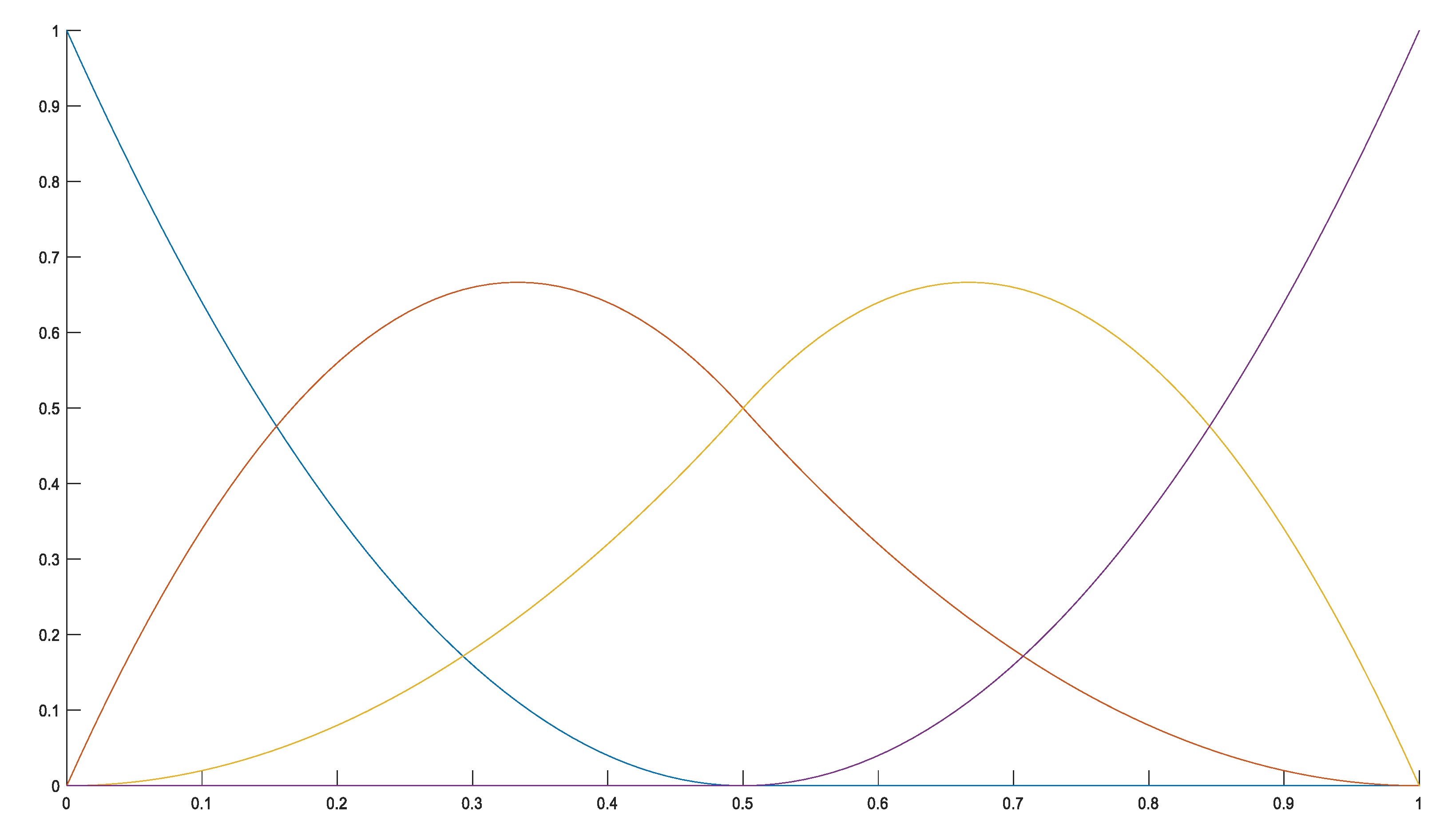
2.1. Curve and Surface Building with B-spline

A linear combination of the shape functions and coefficients denoted by the control points constructs a B-spline curve:

$$C\left(\xi \right)={\displaystyle \sum }_{i=1}^n{N}_{i,p}\left(\xi \right)B_i$$

(4)

$N_{i,p}$ and $B_i$ are the ith B-spline function and control points, respectively.

A B-spline surface is defined by a tensor product and parameterized by two-knot vectors, knot vector = $\left\{\left[{\xi }_1,{\xi }_2,\dots ,{\xi }_{n+p+1}\right],\left[{\eta }_1,{\eta }_2,\dots ,{\eta }_{n+p+1}\right]\right\}$ as:

$$S\left(\xi ,\eta \right)={\sum }_{i=1 }^n{\sum }_{j=1}^m{N}_{i,p}\left(\xi \right)M_{j,q}\left(\eta \right)B_i,$$

(5)

where $N_{i,p}\left(\xi \right) \mathrm{and} M_{j,q}\left(\eta \right)$ are univariate shape functions and B is the 3-vector of control point coordinates.

2.2. Non-Uniform Rational B-splines (NURBS)

NURBS is the generalization of the B-spline functions:

$$R_{i,p}\left(\xi \right)=\frac{N_{i,p}\left(\xi \right) w_i}{{\sum }_{\mathsf{î}=1}^n{N}_{\mathsf{î},p}\left(\xi \right)w_{\mathsf{î}}}$$

(6)

where $w_i$ > 0 is the weighting parameter and $N_{i,p}\left(\xi \right)$ is the B-spline basis function. For $w_i$ = 1, NURBS functions are transformed into B-splines functions. The Rhino Python Editor performs the generation of the weights.

The NURBS shape function’s first derivative with respect to the parameter is:

$$\frac{d}{d\xi }{R}_{i,p}\left(\xi \right)=w_i\frac{W\left(\xi \right)N_{i,p}^{\prime }\left(\xi \right)-W^{\prime }\left(\xi \right)N_{i,p}\left(\xi \right)}{{(W\left(\xi \right))}^2}$$

(7)

where $W\left(\xi \right)$ = ${\sum }_{\mathsf{î}=1}^n{N}_{\mathsf{î},p}\left(\xi \right)$ $w_i$ and $W^{\prime }\left(\xi \right)$ = ${\sum }_{\mathsf{î}=1}^n{N^{\prime }}_{\mathsf{î},p}\left(\xi \right)w_i$.

2.3. Curve and Surface Building with NURBS

To construct the control points for the NURBS geometry, Equation (8) is utilized:

$${(B_i)}_j=\raisebox{1ex}{${(B_i^w)}_j$}\!\left/ \!\raisebox{-1ex}{$w_i$}\right. , j=1,\dots , k$$

(8)

where ${(B_i)}_j$ is the $j^{th}$ element of the vector $B_i$ and $w_i$ the $i^{th}$ weight. By using Equation (6) in combination with Equation (8), the NURBS curve was constructed as:

$$C\left(\xi \right)={\displaystyle \sum }_{i=1}^n{R}_{i,p}\left(\xi \right)B_i$$

(9)

By analogy with the B-spline, NURBS surfaces are constructed from a tensor product through two-knot vector arrays. It is introduced as:

$$S\left(\xi ,\eta \right)={\sum }_{i=1}^n{\sum }_{j=1}^m\frac{N_i^p\left(\xi \right)M_i^q\left(\eta \right)w_{i,j}}{{\sum }_{i=1}^n{\sum }_{j=1}^m{N}_i^p\left(\xi \right)M_i^q\left(\eta \right)w_{i,j}}$$

(10)

The reformulation (10) can be done by setting up in the following form:

$$S\left(\xi ,\eta \right)={\sum }_{i=1}^n{\sum }_{j=1}^m{R}_{i,j}^{p,q}{B}_{i,j}$$

(11)

where $N_i^p\left(\xi \right)$ and $M_i^p\left(\xi \right)$ are shape functions, respectively. Then, p and q are the order of the basis function in the two directions and m and n are the numbers of control points in the two directions.

2.4. Governing Equation

Let us briefly review the concept of discontinuity inside a continuum formulation. The improved displacement field term is introduced, taking into account the displacement field computation at the discontinuity. The concept of the partition of unity has been used for Lagrangian basis functions; the properties of this technique are also suitable for the B-spline and NURBS functions, which form the basis of the iso-geometric approach. The full displacement field can be expressed as the amount of two subfields by using this property:

$$U^h\left(x\right)={\displaystyle \sum }_{I=1}^N{\varphi }_I\left(x\right)\left({\alpha }_I+{\displaystyle \sum }_{J=1}^M{\beta }_{IJ}{K}_J\left(x\right)\right)$$

(12)

In Equation (12), ${\varphi }_I$ represents the standard basis function, $K_J$ is the improved basis function with m expressions, and the standard and the improved nodal degree of freedom are ${\alpha }_I$ and ${\beta }_{IJ}$, respectively. To develop the approximation, M will assume the value 2, and Equation (12) can be represented as:

$$U^h\left(x\right)={\sum }_{I=1}^N{\Phi }_I\left(x\right)\left[{\alpha }_I+H\left(x\right)a_I+{\sum }_{\beta =1}^4{F}_{\beta }\left(x\right)b^{\beta }{}_I\right]$$

(13)

In Equation (13), $K_J$ has been decomposed into two different enrichment terms, the Heaviside function $H\left(x\right)$ and the crack-tip function $F_{\beta }\left(x\right)$, in order to capture the discontinuity and the singular fields. $a_I$ and $b^{\beta }{}_I$ introduce the improved nodal degrees of freedom.

To follow the crack, the level set methodology has been applied. This allows for representing the discontinuity as a moving interface. The signed distance, which defines the location of an arbitrary point with respect to the interface, is still the most popular:

$$\phi \left(x\right)=\parallel x-\hat{x}\parallel \mathrm{sign}\left(n_{{\mathsf{\Gamma }}_d}.\left(x-\hat{x}\right)\right)$$

(14)

where x is a point in a mesh element, $\widehat{x}$ is the closet point to x on the discontinuity, and $n_{{\mathsf{\Gamma }}_d}$ is the interface normal.

The position of the crack in a domain is defined by the values of the level set function that is represented as follows:

$$\phi \left(x\right)=|\begin{array}{c}<0 if x \in {\mathrm{\Gamma }}_d^{-}\\ =0 if x\in {\mathrm{\Gamma }}_d\\ >0 if x \in {\mathrm{\Gamma }}_d^{+}\end{array}$$

(15)

When the body’s forces are not present, the elastostatics equation, in its strongest form, is:

$$\overrightarrow{div} \stackrel{=}{\sigma }=\overrightarrow{ 0} \mathrm{in} \mathsf{\Sigma }$$

(16)

With the appropriate set of boundary conditions:

Essential boundary conditions:

$$\overrightarrow{u}=\overrightarrow{u_D} \mathrm{on} { \mathsf{\Gamma }}_u$$

(17)

Natural boundary conditions:

$$\stackrel{=}{\sigma } \overrightarrow{n}=\overrightarrow{T_D}{ \mathrm{on} \mathsf{\Gamma }}_t$$

(18)

Crack surface:

$$\stackrel{=}{\sigma } {\overrightarrow{n}}_{{\mathsf{\Gamma }}_d}=\overrightarrow{0} \mathrm{on} {\mathsf{\Gamma }}_d$$

(19)

where n is the normal vector, $n_{{\mathsf{\Gamma }}_d}$ is the normal vector regarding the interface (see Figure 2), $\sigma$ is the stress tensor, and u is the displacement vector.

2.5. Variational Formulation

As illustrated in Figure 2, a 2-D domain has been considered in this work with conventional boundary conditions: the Dirichlet ${\mathsf{\Gamma }}_u$ and the Neumann ${\mathsf{\Gamma }}_t$ boundary. The crack face presents further traction-free boundaries ${\mathsf{\Gamma }}_c$.

By using the virtual work theory, the weak form of the problem can be established from the equilibrium equation, and is represented as:

$${ℒ}_{eq}=\underset{\mathsf{\Sigma }}{{\displaystyle \int }}\left(\sigma \left(u\right):\epsilon \left(q\right)\right)d\mathsf{\Sigma }-\underset{\mathsf{\Gamma }}{{\displaystyle \int }}(T_D.q )d\mathsf{\Gamma }$$

(20)

The stress, the strain tensor, and the traction vector are described by $\sigma$, $\epsilon$, and $T_D$, respectively. $u$ and $q$ denote, respectively, the displacement vector and the virtual displacement.

3. Extended Iso-Geometric Analysis (X-IGA)

3.1. X-IGA Formulation for Cracks

X-IGA aims to evaluate fractures in an engineering component without having to re-mesh it. In the framework of the X-FEM approach, the enrichment of the shape functions (B-spline, NURBS) is ensured by a Heaviside and crack-tip function since they constitute a partition unit (PU). The former function was introduced to insert a discontinuity and the latter to treat singularities at the crack tip. The approximation of the solution is given as [54]:

$$U^h\left(\xi \right)={\sum }_{IϵN_{stand}}{R}_I\left(\xi \right)u_I+{\sum }_{JϵN_{CrSplit}}{R}_J\left(\xi \right)H\left(\xi \right)a_J+{\sum }_{KϵN_{CrTip}}{R}_K\left(\xi \right)({\sum }_{\alpha =1}^4{F}_{\alpha }\left(\xi \right)b_K^{\alpha })$$

(21)

where $R_I$ represents shape functions $u_I$, and $a_J$ and $b_K^{\alpha }$ define the standard and the further DOFs, respectively. $N_{stand}$ includes the standard nodes of the mesh, $N_{CrSplit}$ includes the nodes of elements that have been split by the crack faces, and $N_{CrTip}$ includes the nodes of the crack-tip elements. The parameter coordinates are represented by $\xi$. The Heaviside function, wherein the quantities on both parts of the split element are different, is denoted by $H\left(\xi \right)$. The purpose of the crack-tip function, among others, is to increase the accuracy of the results, and it is denoted by $F_{\alpha }$. These enrichment functions are characterized by the following equations [55]:

$$H\left(\xi \right)=\mathrm{sign} \left(\phi \left(\xi \right)\right)=\{\begin{array}{c}-1 if \phi \left(\xi \right)<0\\ +1 if \phi \left(\xi \right)>0\end{array} ,$$

(22)

$$F_{\alpha }\left(\xi \right)=F_{\alpha }\left(r,\theta \right)=\left\{r^{\raisebox{1ex}{$1$}\!\left/ \!\raisebox{-1ex}{$2$}\right.}\left[sin\frac{\theta }{2},cos\frac{\theta }{2},sin\theta sin\frac{\theta }{2},cos\frac{\theta }{2}sin\theta \right]\right\}$$

(23)

The polar coordinates of the crack tip are represented by r,$\theta$.

After substituting Equation (19) in the equilibrium equation, the final phase of the processing stage is to solve the linear algebra system:

$$K^{enr}{U}^{enr}=F^{enr} ,$$

(24)

where $K^{enr}$ denotes an enriched stiffness matrix, $F^{enr}$ denotes a force vector, and $U^{enr}$ denotes an enriched displacement vector as:

$$U^{enr}={\left\{U d b_1 b_2 b_{3 }{b}_4\right\}}^T,$$

(25)

where U is the DOF vector for the IGA normal, d is the DOF for Heaviside enrichment, and $b_1,b_2, b_{3 }, \mathrm{and} b_4$ are the DOF vectors for the crack-tip enrichment functions. $K^{enr}$ and $F^{enr}$ are constructed as follows from the element stiffness matrix:

$$K^{enr}=\left[\begin{array}{cccccc}{K}^{uu}& K^{ua}& K^{u{b}_1}& K^{{ub}_2}& K^{{ub}_3}& K^{{ub}_4}\\ K^{au}& K^{aa}& K^{{ab}_1}& K^{{ab}_2}& K^{{ab}_3}& K^{{ab}_4}\\ K^{b_{1}u}& K^{b_{1}a}& K^{b_1{b}_1}& K^{b_1{b}_2}& K^{b_1{b}_3}& K^{b_1{b}_4}\\ K^{b_{2}u}& K^{b_{2}a}& K^{b_2{b}_1}& K^{b_2{b}_2}& K^{b_2{b}_3}& K^{b_2{b}_4}\\ K^{b_{3}u}& K^{b_{3}a}& K^{b_3{b}_1}& K^{b_3{b}_2}& K^{b_3{b}_3}& K^{b_3{b}_4}\\ K^{b_{4}u}& K^{b_{4}a}& K^{b_4{b}_1}& K^{b_4{b}_2}& K^{b_4{b}_3}& K^{b_4{b}_4}\end{array}\right]$$

(26)

$$F^{enr}={\left\{F^u F^a F^{b_{1 }}{F}^{b_2} F^{b_3} F^{b_4}\right\}}^T.$$

(27)

The number of control points $N_{stand}$, $N_{CrSplit}$, $N_{CrTip}$, and the number of enrichment basis functions $N_{ef}$ determine the size of each $K^{enr}$ and $F^{enr}$. Each component can be written as follows:

$$K_{ij}^{rs}={{\displaystyle \int }}_{{\mathsf{\Sigma }}_e}{\left(B_i^r\right)}^{T}C{B}_j^s d\mathsf{\Sigma } \left(r,s = u, d, b_1, b_2, b_3, b_4\right)$$

(28)

$$F_i^u={{\displaystyle \int }}_{{\mathsf{\Gamma }}_u}{R}_i^T{T}_{D}d\mathsf{\Gamma },$$

(29)

$$F_i^a={{\displaystyle \int }}_{{\mathsf{\Gamma }}_t}{R}_i^{T}H{T}_{D}d\mathsf{\Gamma },$$

(30)

$$F_i^{b_{\alpha }}={{\displaystyle \int }}_{{\mathsf{\Gamma }}_t}{R}_i^T{f}_{b_{\alpha }}{T}_{D}d\mathsf{\Gamma } \left(\alpha =1, 2, 3, 4\right)$$

(31)

$$B_i^u=\left[\begin{array}{cc}\frac{\partial R_i}{\partial x}& 0\\ 0& \frac{\partial R_i}{\partial y}\\ \frac{\partial R_i}{\partial y}& \frac{\partial R_i}{\partial x}\end{array}\right]$$

(32)

$$B_i^a=\left[\begin{array}{cc}\frac{\partial R_i}{\partial x}H& 0\\ 0& \frac{\partial R_i}{\partial y}H\\ \frac{\partial R_i}{\partial y}H& \frac{\partial R_i}{\partial x}H\end{array}\right]$$

(33)

$$B_i^{b_{\alpha }}=\left[\begin{array}{cc}\frac{\partial R_i{f}_{b_{\alpha }}}{\partial x}& 0\\ 0& \frac{\partial R_i{f}_{b_{\alpha }}}{\partial y}\\ \frac{\partial R_i{f}_{b_{\alpha }}}{\partial y}& \frac{\partial R_i{f}_{b_{\alpha }}}{\partial x}\end{array}\right] \left(\alpha =1, 2, 3, 4\right)$$

(34)

The Heaviside function (Equation (22)) is represented by H, while the crack-tip enrichment function (Equation(23)) is represented by $f_{b_{\alpha }}$.

3.2. Construction of 2-D Pipe with X-IGA Concept

A patch with an internal interface is used to model a 2-D pipe problem (Figure 3); this interface is the result of coinciding control points in the circumferential direction at the beginning and end of the patch. To solve the problem correctly, we must confine the control values of these overlapping control points so that each pair of control values for the corresponding coincident control points is the same. The master–slave approach is a simple solution to this problem. This method is implemented in the present study by the global renumbering of DOFs in the physical space, where coincident DOFs are numbered by the same indices. The global numbering is saved in an array and given as an additional input argument.

3.3. Enrichment Topology for Control Points

In IGA, every basis function is linked to its corresponding control point in a specific way. The intersection of each supported domain with the crack face leads to enrichment by the Heaviside function. The domain support, which contains the crack tip, will be enriched by the singular function. According to [56], there are two ways to enrich the crack tip: with either topological or geometrical enrichment. In this work, topological enrichment has been employed. Figure 4 shows a schematic representation of this concept.

According to the Figure 4, $C_s$ denotes the crack-face control points, while $C_T$ denotes the crack-tip-enriched control points, and $C_i$ denotes the standard control point. For the purpose of selecting enriched control points, the level set method has been used. We applied the procedure that has been used by [58]. Initially, the level set values of the crack at the mesh’s vertices are computed according to these level sets, and the formulation determines the elements intersected by the crack and the crack-tip element.

4. Numerical Integration in the Elastic Field

For numerical integration, the standard Gaussian quadrature method cannot be applied explicitly to the XIGA since it contains various discontinuous elements. To assess the integration rule of the crack’s split and tip elements in this study, the triangular sub-domain methodology is used (Figure 5). This technique has been successfully implemented by X-FEM [42], as seen in Figure 6. Each sub-triangle element has a defined number of integration points.

5. Fracture Parameter Evaluation

The stress intensity factor (SIF) is a crucial criterion in crack formation and growth research. As a result, when a numerical simulation is used to solve fracture mechanics issues, one of the objectives is to quantify the SIF. There are a range of ways to calculate this parameter, which is used in so much of the interaction integral method [55]:

$$M=\underset{\mathrm{\Gamma }}{{\displaystyle \int }}\left[{\sigma }_{ij}^{act}\frac{\partial u_i^{aux}}{\partial x_1}+{\sigma }_{ij}^{aux}\frac{\partial u_i^{act}}{\partial x_1}-W^M{\delta }_{1j}\right]\frac{\partial q}{\partial x_j}d\mathrm{\Gamma },$$

(35)

where M is the interaction integral with the aux and act index defining the auxiliary and the actual state, respectively. The stress and the displacement are represented by ${\sigma }_{ij}$ and $u_i$, respectively. $W^M$ represents the interaction work; it can be described in the following form:

$$W^M=\frac{1}{2}\left({\sigma }_{ij}^{act}{\epsilon }_{ij}^{aux}+{\sigma }_{ij}^{aux}{\epsilon }_{ij}^{act}\right),$$

(36)

where ${\epsilon }_{ij}$ and $q$ define the strain and an arbitrary function, whose values are defined as:

$$q=\{\begin{array}{cc}\hfill 1,\mid & at the crack tip\hfill \\ \hfill 0,\mid & along the contour\hfill \end{array}$$

(37)

The stress intensity factor with these two modes (I, II) and the J-integral are related by:

$$J=\frac{1}{E^{\prime }}\left(K_I^2+K_{II}^2\right).$$

(38)

Based on this correlation, the following equation has been derived:

$$M=\frac{2}{E^{\prime }}\left(K_I^{act}{K}_I^{aux}+K_{II}^{act}{K}_{II}^{aux}\right)$$

(39)

where

$$E^{\prime }=\{\begin{array}{c} E for plane stress\\ \frac{E}{1-{\nu }^2} for plane strain\end{array}$$

(40)

E represents the Young’s Modulus, v is the Poisson’s ratio, and M represents the interaction integral.

The crack opening is the field of interest of this study. Therefore, the SIF in mode I can be obtained by choosing $K_I^{aux}$=1 and $K_{II}^{aux}=0$. Finally, the SIF is defined as:

$$K_I=\frac{E^{\prime }}{2}M$$

(41)

6. Process of Implementing a X-FEM Code in ABAQUS

The idea of implementing the X-FEM technique is based on the fact that the ABAQUS software does not include the stress intensity factor computation for a 2-D crack. The two enriched functions that correspond to the Heaviside and the crack-tip functions that appeared in Equation (13) were implemented through a user-defined element (UEL). The implementation process requires three phases: pre-processing, processing, and post-processing. In this study, to make the implementation easier, the input file (XFEM.inp) has been generated by ABAQUS, and then the interaction between the crack and the mesh was constructed to apply Equation (14). Therefore, the enriched elements and nodes have been determined. The user-defined element (UEL) in ABAQUS is used to program the processing stage (UEL.for) to compute the stresses and strains. The last stage consists of calculating the Mode-I SIF, KI, by a post-processing code; indeed, the interaction integral method explained in section five (Fracture Parameter Evaluation) has been programmed in FORTRAN. The details for the file descriptions are based on [53], who introduce the X-FEM implementation in ABAQUS. Thus, we have adopted the principle of this implementation for our problem. The ABAQUS command is used to run the main file (XFEM.inp) and the user subroutine file (UEL.for): Abaqus job = X-FEM user = UEL.for.

The resulting information of this simulation is stored in (XFEM.fil), and the ABAQUS output conventions are included in this file. Then, we used an external subroutine for computing the stress intensity factors. This subroutine is compiled through the ABAQUS command “ABAQUS make job = interaction_integral”, and then run with the command “ABAQUS interaction_integral”. The implementation process is described in Figure 7.

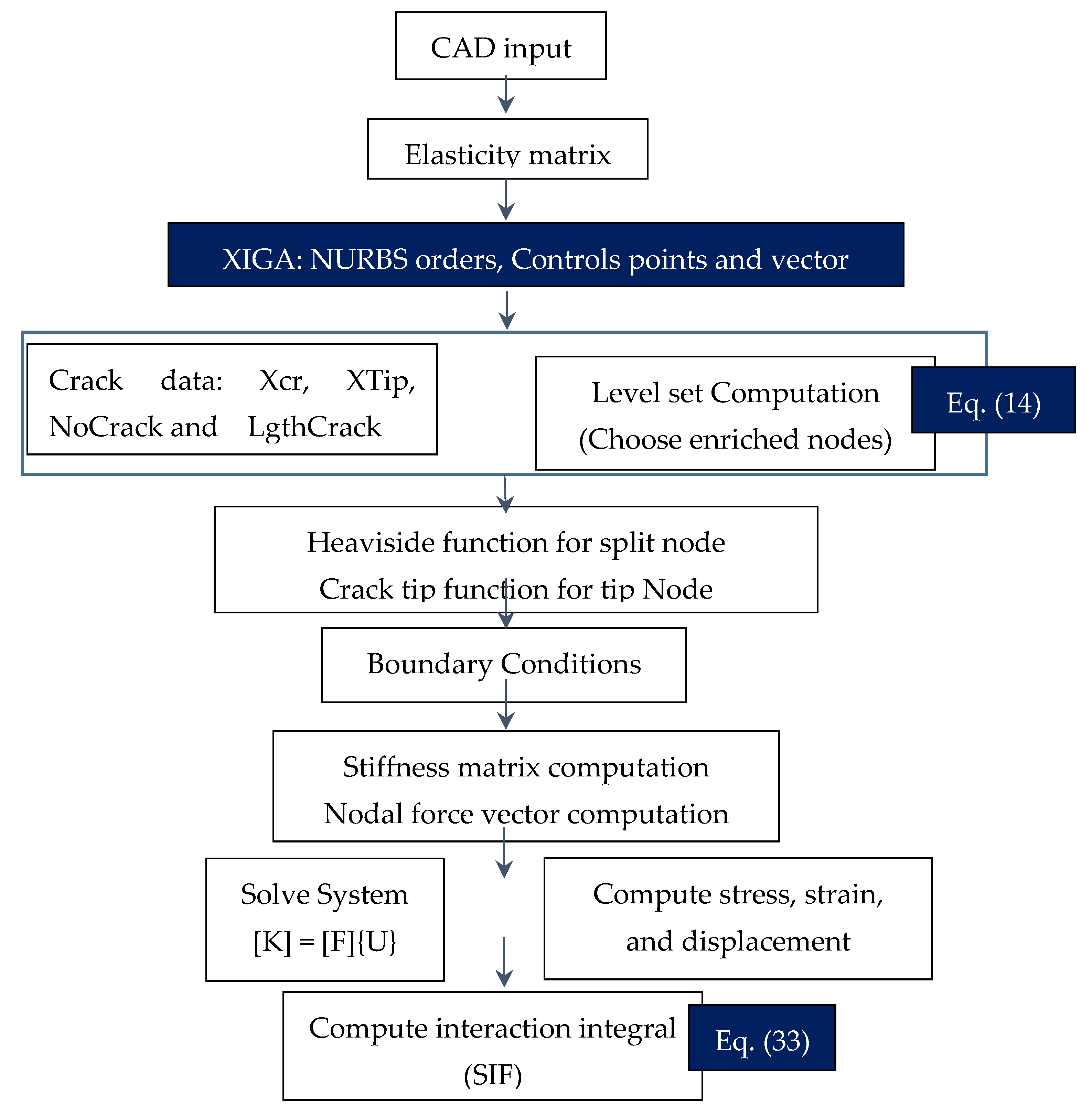
7. Process of Implementing a X-IGA Code in MATLAB

In this section, the main steps of the XIGA implementation code to numerically model a structure with a pre-existing discontinuity (a crack) have been summarized in Figure 8. To understand the implementation, it is necessary to know two major things: the three steps of a finite element code (pre-processing, processing, and post-processing), and the identification of a crack using the level set method (LSM). The flowchart starts with the introduction of the input parameters, which contain the geometrical data and the material properties. Then, the elasticity matrix is integrated. In addition, the data required by the NURBS functions, such as the polynomial order, control points, and node vectors, are introduced to build the NURBS model. The next step is to introduce the crack data, length, and coordinates of the crack points with the level set method to determine the position of the crack and to select the enrichment points. Then, the Heaviside and crack-tip functions are imposed on the nodes according to the technique that precedes this step. Then, the boundary conditions, nodal force vector, and stiffness matrix are calculated. The stress, strain, and displacement values are the output of this process. These data can be put to use in the interaction integral to compute the stress intensity factor.

8. Numerical Results and Discussions

The iso-geometric analysis is extended and used in this section to analyze the cracked model under mechanical loading; a specimen from the industrial field is chosen. Pressure pipes are commonly used and the performance of these systems is still under investigation. In a 2-D linear static analysis case, an isotropic and homogeneous pipe has been studied. The plane stress is thought to be the stress distribution state. For this analysis, The P264GH material is used and its mechanical and chemical characteristics are described in

Table 1. Mechanical characteristics for the P264GH [59].

Properties	Values
Young’s Modulus	207 GPa
Poisson ratio	0.3
Yield Stress	340 MPa
Ultimate tensile strength	440 MPa
Elongation to fracture	35%
Fracture Toughness	95 $\mathrm{MPa}\sqrt{\mathrm{m}}$

and

Table 2. Chemical characteristic of P264GH—% by weight [60].

Material	C	P	Al	Mn	S	Si	Fe
Tested steel	0.135	0.013	0.027	0.665	0.002	0.195	Bal.
P264GH steel according to the Standard EN10028.2-92	0.18	0.025	0.02	1	0.015	0.4	Bal.

, respectively.

To examine the reliability, accuracy, and efficiency of this approach, an external axial crack was studied. The results of the analysis were compared with the results of standard ABAQUS software using the classical finite element method (CFEM), which is based on the integral contour and the X-FEM method using a subroutine UEL code.

In each of these parametric directions $\xi$ and $\eta$, the degree of the NURBS polynomial is two (p = q = 2). In the first direction $\xi$, the knot vector is open and with interior duplication, and in the second direction $\eta$, the knot vector is open and without internal duplication.

The integration is done along each Gauss point direction (p + 1) × (q + 1), and as the sub-triangles approach was used in this case, 13 Gauss quadrature points were imposed for each sub-triangle. For each numerical method, different mesh sizes were examined. It is important to be aware that the crack was represented as a straight segment.

In order to figure out the fracture parameter, i.e., to estimate the stress state near a crack tip, the stress intensity factor (SIF), KI, and the J-Integral are extracted. For the three techniques used in this work, the interaction integral method was implemented. The X-IGA technique was implemented in MATLAB code. The ABAQUS software was used for the CFEM and X-FEM to extract the KI, but for the X-FEM, it is important to mention that the software does not support the computation of this parameter in the 2-D domain, which led to the use of a subroutine UEL.

8.1. Two-Dimensional Pipe with an Axial Crack under Uniform Pressure

In the present study, an isotropic and homogenous 2-D pipe including a 2 mm straight edge crack with uniform pressure distribution and an outer and inner radius of Ro=20 mm and Ri=10 mm, respectively, is examined. Three models were used in this study, which included 320, 480, and 640 element numbers for the X-IGA method, and 1297, 3844, and 85,942 element numbers for the CFEM, with a step size of 1, 0.5, and 0.1, respectively, and 470, 1265, and 2747 element numbers for X-FEM with a step size of 1, 0.45, and 0.25 around the crack, respectively. The NURBS geometry is represented by using several patches (subdomains) with an internal interface. In the circumferential direction, the control points coincide with each other on the patch, and this implies the creation of interface terms. The NURBS geometry is illustrated in Figure 9a.

The FEM model has been represented by a finite element mesh on ABAQUS software. The most important thing is that the modeling of the crack requires a specific treatment, i.e., it requires building a particular mesh around the crack. A ring of a triangle, as represented in Figure 9b, is formed at the crack tip, along with concentric layers of structured quads [61].

For the X-FEM method (Figure 9c), the meshing was done in a simple way since the crack was modeled independently of the meshing. It should be noted that, for this technique, a half tube was treated because the implementation is heavy when using UEL subroutines, so to overcome this problem, a half tube was analyzed with the symmetry boundary conditions.

To perform the numerical simulation, we present

Table 3. Data details for the numerical simulation.

Crack Length Ratios (a/t)	Crack Position (x1 y1; x2 y2) (mm)	Applied Pressure (MPa)
0.2, 0.3, 0.4, 0.5, 0.6, 0.7, 0.8	(−20 0; (−20 + a) 0)	2.5

, which summarizes the crack length, crack position, and pressures applied.

Figure 10 illustrates the distribution of the Von Mises stress by the three techniques for $\raisebox{1ex}{$a$}\!\left/ \!\raisebox{-1ex}{$t$}\right.=0.3$, and a pressure of 2.5 MPa [52] has been applied. The accuracy of the stress and strain distribution in a geometry takes a very important place in fracture mechanics, especially when it concerns cracking problems.

The zone of interest is the crack tip where the degree of damage of the defect has been known. Obtaining a regularity of stresses in this region is a priority for numerical methods since the calculation of fracture parameters, such as the stress intensity factor, as well as the angle of deviation of the crack propagation, is based on the value of stresses at the crack tip.

By comparison of the three results of Figure 10, there is a similarity in the results of the numerical simulation. However, some errors can appear when using these numerical techniques. The errors’ origins are detailed as follows: with the CFEM analysis, the field of strains and stresses become singular at the crack tip, even with the integration of the singularity in the model to improve the accuracy of the results. With the implementation of the X-FEM method via user subroutine UEL in ABAQUS, a mesh sensitivity affects the simulation results. For the present study, there is no singularity at the crack tip and there is a minor sensitivity of mesh. The next section of this work shows a calculation of different meshes for all the different methods. The X-IGA method implemented in MATLAB can be an alternative to these numerical methods. The results presented in Figure 10 can support this conclusion because 4112 elements were used for the full tube with the CFEM method, 2747 elements for the half tube with the X-FEM method, and only 384 elements for the XIGA method. For this reason, the evaluation of the stresses around an existing crack on a pipe can be made by the present study with large elements and with a weak error, which appears in the solution discretization.

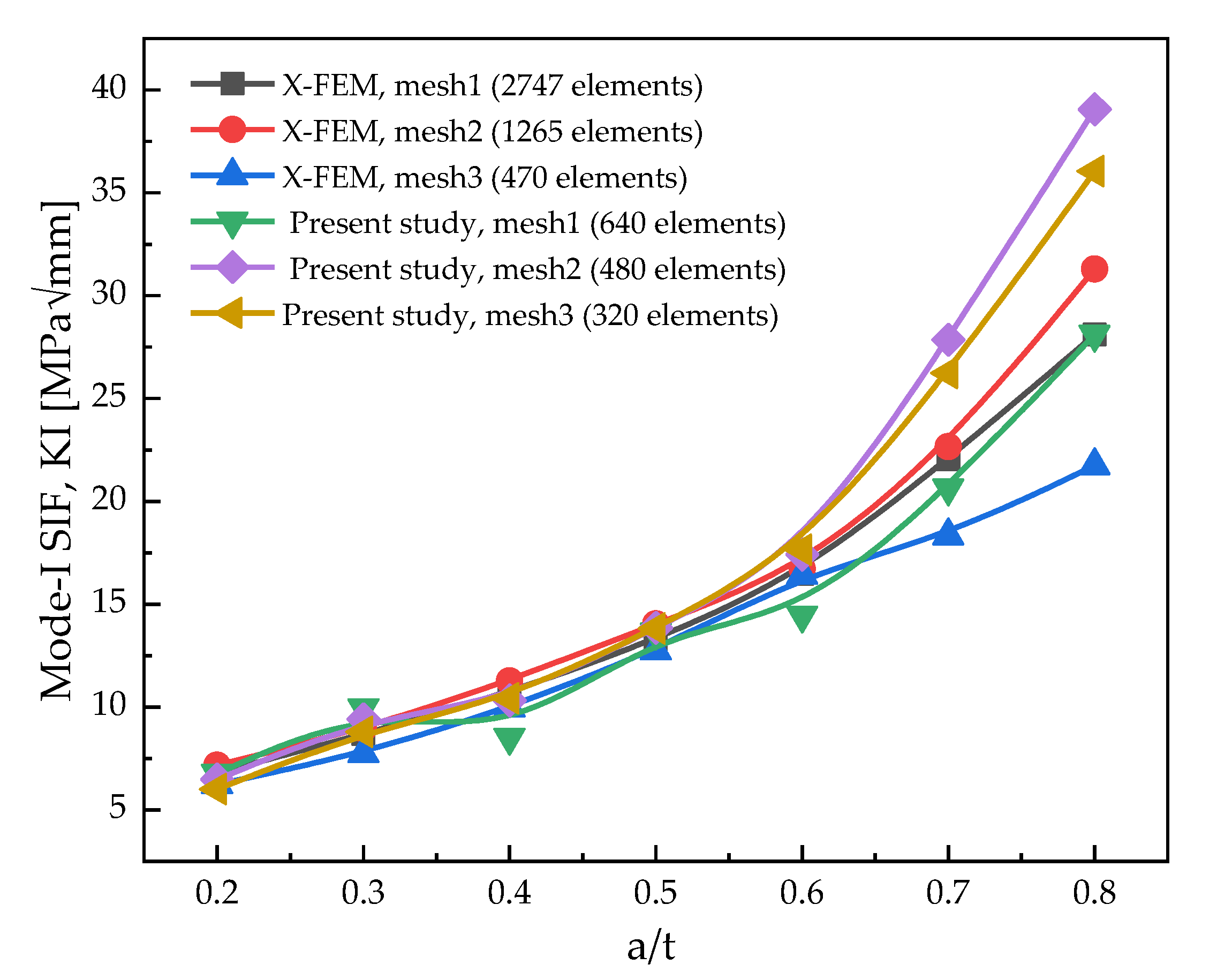
8.2. Evaluation of the Fracture Parameter

In order to present the accuracy of the X-IGA technique, as well as the regularity of the stress distribution around the crack tip, the SIFs were extracted and the value of the mode I (K_I) was calculated in this study, since the degree of damage that corresponds to the opening of the crack is more severe than with the other modes [62]. To ensure that this study is inscribed in linear elasticity, a pressure of 2.5 MPa [52] was applied. Three models are evaluated for different mesh sizes. Therefore, the result of CFEM, X-FEM, and X-IGA are compared. Moreover, the interaction integral approach, which is known as M-integral, was used for calculating the SIFs.

For this comparison, the depth of the crack was varied from the thickness of the model a/t; the thickness is t = 10 mm and a = 2, 3, …, 8 mm. Figure 11 and Figure 12 illustrate the results of the computation. The comparison between the results obtained by the X-IGA and CFEM methods shows a good similarity. It is observed that fine meshes must be used to discretize the areas around the crack tips for the CFEM, whereas the meshes are coarser for the XIGA. It is clear to observe that only 640 elements are required by the present study to obtain the result of 1297 elements with the CFEM method. Results obtained by implementing X-IGA in MATLAB are in good agreement with the CFEM method implemented in ABAQUS. The mentioned technique did not require much effort in dealing with the mesh in the crack tip, whereas using ABAQUS required a specific meshing technique, due to the singularity at the crack tip, and this can affect the numerical results.

As for the comparison between the X-IGA and X-FEM, the results show a good similarity. It is also observed that, with X-FEM, a fine mesh must be used without a particular treatment around the crack, since the crack is modelled independently of the mesh. It is clear to observe that the present study requires just 640 elements for obtaining the result of 2747 elements using X-FEM. The same enrichment functions for overcoming the problem of singularity are used for both methods and only the shape functions are modified. Therefore, there is a similarity of results between the two numerical methods. When the depth of the crack approaches the inside of the pipe, the SIFs values become maximized. It is clear to see that whatever technique is employed to simulate the crack, the SIFs gradually increase with the crack length.

By these results, implementing X-IGA in MATLAB shows the possibility to calculate the fracture mechanics parameters for a cracked pipe under uniform pressure with a large mesh size, compared to the other approaches (Figure 12). Therefore, it can be an alternative way to evaluate the damage of a cracked pipe.

In addition to the SIF, the J-integral has specific importance when it comes to the numerical stress analysis of cracks. To give more physical meaning to the analysis, and to validate the strategy used in the application of X-IGA to address the cracking pipe problem, we evaluated the J-integral with various crack lengths, as shown in Figure 13. Here, we used 640 elements for the present study, and 2747 and 85,642 elements for X-FEM and CFEM, respectively. The J-integral value increased gradually with the crack length and the results obtained are similar to other numerical results.

This problem is also analyzed by [51]; they used a UEL subroutine in the ABAQUS software to evaluate the stress intensity factor. With the same element number and for a = 5 mm and p = 2.5 MPa, we evaluated the performance of the present study and the results of both implementations are compared with Folias solutions [63], as illustrated in

Table 4. Comparative study of the present investigation and implementation using Fortran for a = 5 mm.

Method/ Implementation	X-IGA/ Fortran [51]	XIGA/ Fortran [51]	Present Study MATLAB	Present Study MATLAB	Folias Solution [63]
Element Number	470	767	470	767	______
KI (MPa$\sqrt{\mathrm{mm}}$)	13.18	13.015	13.85	13.51	14.37
Error (%)	8.306	9.454	3.645	6.01

.

Table 3 proves the significance of the present study implemented in MATLAB. It is interesting to note that, in the present study, the error for a model with 470 elements is 3.645%, while for the study implemented in Fortran the error is 8.306%. Additionally, with 767 elements, the error for the present study is 6.01%, while for the study implemented in Fortran the error is 9.454%. It is observed that the X-IGA implementation strategy that was followed in the present study had a higher accuracy than the strategy followed by [51].

In addition, the accuracy of the present study can be realized by computing the error of SIFs (%) with various crack lengths, as illustrated in Figure 14. It is noted that the maximum error of the present study is 12.25%, while the study implemented in Fortran [51] is 27.83%.

8.3. Effect of Pressure on the Fracture Parameter Calculation

Finally, in order to check the efficiency of the present study for the calculation of the fracture parameter in the 2-D pipe domain, the inner pressure was varied with the initial crack length a = 4 mm, so that the pressure did not exceed 4.5 MPa [64], keeping the analysis in the elastic domain. The results of the SIFs and the J-Integral of CFEM, X-FEM, and X-IGA are presented in Figure 15. It is observed that for the three-analyses technique, the stress intensity factor increases with the increase of inner pressure. It is also observed that the results for both the X-FEM and X-IGA methods became similar each time the pressure was increased; this is due to the use of enrichment functions at the crack tip. The singularity at the crack tip and the mesh dependency for the CFEM method makes their results inaccurate.

From these results, the X-IGA method can be used in the fracture parameters computation on cracked cylindrical structures under uniform pressure, the X-IGA method has been well validated for the calculation of cracked plates [48], and this study is an extension of the research work that has already been done in this field. The comparison between the most-known methods in the field of numerical computation will allow us to justify the role of this new technique: it can replace the existing methods in the current calculation codes in the future, and the validation of the efficiency of this technique by the different research works will convince the users in the industrial field. This is due to several reasons; the most important reason, for the industrial sector, is the cost of calculation. Instead of designing the model and approximating it by several meshing processes, it is enough to use the geometry directly by the same shape functions, named B-spline or NURBS; after that, the model will be reproduced precisely. It has been observed that X-IGA just needs a small element for a crack in a pipe, compared to other techniques, and that with these elements, the same results have been obtained, so if there is a complex geometry, the calculation procedure will be very fast compared to the current method.

9. Conclusions

The aim of this investigation was to implement the X-IGA technique into a MATLAB code for modeling cracked pipelines. The main theoretical approach was the NURBS principle, which provided a higher-order continuity in numerical modeling.

An external crack in a two-dimensional pipe subjected to a uniform pressure has been studied. The accuracy of this technique has been examined by deriving the stress intensity factors and the J-integral. For several mesh sizes and for different inner pressures, SIFs and the J-integral were extracted by X-IGA analysis using MATLAB code and its accuracy was validated with the enrichment technique (X-FEM) using FORTRAN language and the conventional finite element method (X-FEM) using ABAQUS software. It has been shown that, when using the X-IGA analysis:

• The cracked pipe modeling does not need a finer mesh than other numerical techniques. Therefore, the cost of computational will be reduced;
• The regularity of the stress and strain at the crack tip is obtained;
• The geometry was constructed exactly with using NURBS, which avoids the discretization error. Therefore, confident results can be achieved;
• The error on the SIFs is minimal compared to X-IGA implemented by FORTRAN.

Other problems can be addressed by the provided technique, such as crack-growth problems and dynamic fracture analyses in pipelines, which are planned for future research.

References

1. Barsoum, R.S. On the Use of Isoparametric Finite Elements in Linear Fracture Mechanics. Int. J. Numer. Methods Eng. 1976, 10, 25–37. [Google Scholar] [CrossRef]
2. Cheung, S.; Luxmoore, A.R. A Finite Element Analysis of Stable Crack Growth in an Aluminium Alloy. Eng. Fract. Mech. 2003, 70, 1153–1169. [Google Scholar] [CrossRef]
3. Pasetto, M.; Baek, J.; Chen, J.-S.; Wei, H.; Sherburn, J.A.; Roth, M.J. A Lagrangian/Semi-Lagrangian Coupling Approach for Accelerated Meshfree Modelling of Extreme Deformation Problems. Comput. Methods Appl. Mech. Eng. 2021, 381, 113827. [Google Scholar] [CrossRef]
4. Moës, N.; Belytschko, T. Extended Finite Element Method for Cohesive Crack Growth. Eng. Fract. Mech. 2002, 69, 813–833. [Google Scholar] [CrossRef] [Green Version]
5. Montassir, S.; Yakoubi, K.; Moustabchir, H.; Elkhalfi, A.; Rajak, D.K.; Pruncu, C.I. Analysis of Crack Behaviour in Pipeline System Using FAD Diagram Based on Numerical Simulation under XFEM. Appl. Sci. 2020, 10, 6129. [Google Scholar] [CrossRef]
6. Yakoubi, K.; Montassir, S.; Moustabchir, H.; Elkhalfi, A.; Pruncu, C.I.; Arbaoui, J.; Farooq, M.U. An Extended Finite Element Method (XFEM) Study on the Elastic T-Stress Evaluations for a Notch in a Pipe Steel Exposed to Internal Pressure. Mathematics 2021, 9, 507. [Google Scholar] [CrossRef]
7. Yang, L.; Yang, Y.; Zheng, H. A Phase Field Numerical Manifold Method for Crack Propagation in Quasi-Brittle Materials. Eng. Fract. Mech. 2021, 241, 107427. [Google Scholar] [CrossRef]
8. Partridge, P.W.; Brebbia, C.A. Dual Reciprocity Boundary Element Method; Springer Science & Business Media: Berlin/Heidelberg, Germany, 2012; ISBN 94-011-3690-4. [Google Scholar]
9. Bazazzadeh, S.; Mossaiby, F.; Shojaei, A. An Adaptive Thermo-Mechanical Peridynamic Model for Fracture Analysis in Ceramics. Eng. Fract. Mech. 2020, 223, 106708. [Google Scholar] [CrossRef]
10. Daux, C.; Moës, N.; Dolbow, J.; Sukumar, N.; Belytschko, T. Arbitrary Branched and Intersecting Cracks with the Extended Finite Element Method. Int. J. Numer. Methods Eng. 2000, 48, 1741–1760. [Google Scholar] [CrossRef]
11. Belytschko, T.; Black, T. Elastic Crack Growth in Finite Elements with Minimal Remeshing. Int. J. Numer. Methods Eng. 1999, 45, 601–620. [Google Scholar] [CrossRef]
12. Andrade, H.; Leonel, E. An Enriched Dual Boundary Element Method Formulation for Linear Elastic Crack Propagation. Eng. Anal. Bound. Elem. 2020, 121, 158–179. [Google Scholar] [CrossRef]
13. Bhardwaj, G.; Singh, I.; Mishra, B.; Bui, T. Numerical Simulation of Functionally Graded Cracked Plates Using NURBS Based XIGA under Different Loads and Boundary Conditions. Compos. Struct. 2015, 126, 347–359. [Google Scholar] [CrossRef]
14. Hughes, T.J.; Cottrell, J.A.; Bazilevs, Y. Isogeometric Analysis: CAD, Finite Elements, NURBS, Exact Geometry and Mesh Refinement. Comput. Methods Appl. Mech. Eng. 2005, 194, 4135–4195. [Google Scholar] [CrossRef] [Green Version]
15. Benson, D.; Bazilevs, Y.; Hsu, M.-C.; Hughes, T. A Large Deformation, Rotation-Free, Isogeometric Shell. Comput. Methods Appl. Mech. Eng. 2011, 200, 1367–1378. [Google Scholar] [CrossRef]
16. Chen, Y.; Lin, S.; Faruque, O.; Alanoly, J.; El-Essawi, M.; Baskaran, R. Current Status of Lsdyna Isogeometric Analysis in Crash Simulation. In Proceedings of the 14th International LS-DYNA Conference, Detroit, MI, USA, 12–14 June 2016. [Google Scholar]
17. Latimer, C.; Kópházi, J.; Eaton, M.; McClarren, R. Spatial Adaptivity of the SAAF and Weighted Least Squares (WLS) Forms of the Neutron Transport Equation Using Constraint Based, Locally Refined, Isogeometric Analysis (IGA) with Dual Weighted Residual (DWR) Error Measures. J. Comput. Phys. 2021, 426, 109941. [Google Scholar] [CrossRef]
18. Occelli, M.; Elguedj, T.; Bouabdallah, S.; Morançay, L. LR B-Splines Implementation in the Altair RadiossTM Solver for Explicit Dynamics IsoGeometric Analysis. Adv. Eng. Softw. 2019, 131, 166–185. [Google Scholar] [CrossRef]
19. Elguedj, T.; Duval, A.; Maurin, F.; Al-Akhras, H. Abaqus User Element Implementation of NURBS Based Isogeometric Analysis. In Proceedings of the 6th European Congress on Computational Methods in Applied Sciences and Engineering, Vienna, Austria, 10–14 September 2012; pp. 10–14. [Google Scholar]
20. Duval, A.; Elguedj, T.; Al-Akhras, H.; Maurin, F. AbqNURBS: Implémentation D’éléments Isogéométriques Dans Abaqus et Outils de Pré-et Post-Traitement Dédiés; CSMA: Giens, France, 2015. [Google Scholar]
21. Lai, Y.; Zhang, Y.J.; Liu, L.; Wei, X.; Fang, E.; Lua, J. Integrating CAD with Abaqus: A Practical Isogeometric Analysis Software Platform for Industrial Applications. Comput. Math. Appl. 2017, 74, 1648–1660. [Google Scholar] [CrossRef]
22. Xue, Y.; Jin, G.; Ding, H.; Chen, M. Free Vibration Analysis of In-Plane Functionally Graded Plates Using a Refined Plate Theory and Isogeometric Approach. Compos. Struct. 2018, 192, 193–205. [Google Scholar] [CrossRef]
23. Chen, D.; Zheng, S.; Wang, Y.; Yang, L.; Li, Z. Nonlinear Free Vibration Analysis of a Rotating Two-Dimensional Functionally Graded Porous Micro-Beam Using Isogeometric Analysis. Eur. J. Mech. -A/Solids 2020, 84, 104083. [Google Scholar] [CrossRef]
24. Kamensky, D. Open-Source Immersogeometric Analysis of Fluid–Structure Interaction Using FEniCS and TIGAr. Comput. Math. Appl. 2021, 81, 634–648. [Google Scholar] [CrossRef]
25. Simona, A.; Bonaventura, L.; de Falco, C.; Schöps, S. IsoGeometric Approximations for Electromagnetic Problems in Axisymmetric Domains. Comput. Methods Appl. Mech. Eng. 2020, 369, 113211. [Google Scholar] [CrossRef]
26. Bucelli, M.; Salvador, M.; Quarteroni, A. Multipatch Isogeometric Analysis for Electrophysiology: Simulation in a Human Heart. Comput. Methods Appl. Mech. Eng. 2021, 376, 113666. [Google Scholar] [CrossRef]
27. Rouwane, A.; Bouclier, R.; Passieux, J.-C.; Périé, J.-N. Adjusting Fictitious Domain Parameters for Fairly Priced Image-Based Modeling: Application to the Regularization of Digital Image Correlation. Comput. Methods Appl. Mech. Eng. 2021, 373, 113507. [Google Scholar] [CrossRef]
28. Du, X.; Zhao, G.; Wang, W.; Guo, M.; Zhang, R.; Yang, J. NLIGA: A MATLAB Framework for Nonlinear Isogeometric Analysis. Comput. Aided Geom. Des. 2020, 80, 101869. [Google Scholar] [CrossRef]
29. Benson, D.; Bazilevs, Y.; Hsu, M.-C.; Hughes, T. Isogeometric Shell Analysis: The Reissner–Mindlin Shell. Comput. Methods Appl. Mech. Eng. 2010, 199, 276–289. [Google Scholar] [CrossRef] [Green Version]
30. Mi, Y.; Yu, X. Isogeometric MITC Shell. Comput. Methods Appl. Mech. Eng. 2021, 377, 113693. [Google Scholar] [CrossRef]
31. Sobhani, E.; Masoodi, A.R.; Ahmadi-Pari, A.R. Vibration of FG-CNT and FG-GNP Sandwich Composite Coupled Conical-Cylindrical-Conical Shell. Compos. Struct. 2021, 273, 114281. [Google Scholar] [CrossRef]
32. Sobhani, E.; Moradi-Dastjerdi, R.; Behdinan, K.; Masoodi, A.R.; Ahmadi-Pari, A.R. Multifunctional Trace of Various Reinforcements on Vibrations of Three-Phase Nanocomposite Combined Hemispherical-Cylindrical Shells. Compos. Struct. 2021, 279, 114798. [Google Scholar] [CrossRef]
33. Rezaiee-Pajand, M.; Masoodi, A.R. Analyzing FG Shells with Large Deformations and Finite Rotations. World J. Eng. 2019, 16, 636–647. [Google Scholar] [CrossRef]
34. Marathe, S.P.; Raval, H.K. Numerical Investigation on Forming Behavior of Friction Stir Tailor Welded Blanks (FSTWBs) during Single-Point Incremental Forming (SPIF) Process. J. Braz. Soc. Mech. Sci. Eng. 2019, 41, 424. [Google Scholar] [CrossRef]
35. Temizer, I.; Wriggers, P.; Hughes, T. Contact Treatment in Isogeometric Analysis with NURBS. Comput. Methods Appl. Mech. Eng. 2011, 200, 1100–1112. [Google Scholar] [CrossRef]
36. Dimitri, R.; Zavarise, G. Isogeometric Treatment of Frictional Contact and Mixed Mode Debonding Problems. Comput. Mech. 2017, 60, 315–332. [Google Scholar] [CrossRef]
37. Wang, Y.; Wang, Z.; Xia, Z.; Poh, L.H. Structural Design Optimization Using Isogeometric Analysis: A Comprehensive Review. Comput. Modeling Eng. Sci. 2018, 117, 455–507. [Google Scholar] [CrossRef] [Green Version]
38. Yu, T.; Yin, S.; Bui, T.Q.; Liu, C.; Wattanasakulpong, N. Buckling Isogeometric Analysis of Functionally Graded Plates under Combined Thermal and Mechanical Loads. Compos. Struct. 2017, 162, 54–69. [Google Scholar] [CrossRef]
39. Kaushik, V.; Ghosh, A. Experimental and XIGA-CZM Based Mode-II and Mixed-Mode Interlaminar Fracture Model for Unidirectional Aerospace-Grade Composites. Mech. Mater. 2021, 154, 103722. [Google Scholar] [CrossRef]
40. Melenk, J.M.; Babuška, I. The Partition of Unity Finite Element Method: Basic Theory and Applications. Comput. Methods Appl. Mech. Eng. 1996, 139, 289–314. [Google Scholar] [CrossRef] [Green Version]
41. De Luycker, E.; Benson, D.J.; Belytschko, T.; Bazilevs, Y.; Hsu, M.C. X-FEM in Isogeometric Analysis for Linear Fracture Mechanics. Int. J. Numer. Methods Eng. 2011, 87, 541–565. [Google Scholar] [CrossRef] [Green Version]
42. Ghorashi, S.S.; Valizadeh, N.; Mohammadi, S. Extended Isogeometric Analysis for Simulation of Stationary and Propagating Cracks. Int. J. Numer. Methods Eng. 2012, 89, 1069–1101. [Google Scholar] [CrossRef]
43. Bhardwaj, G.; Singh, I.; Mishra, B. Numerical Simulation of Plane Crack Problems Using Extended Isogeometric Analysis. Procedia Eng. 2013, 64, 661–670. [Google Scholar] [CrossRef] [Green Version]
44. Singh, S.; Singh, I.V.; Bhardwaj, G.; Mishra, B. A Bézier Extraction Based XIGA Approach for Three-Dimensional Crack Simulations. Adv. Eng. Softw. 2018, 125, 55–93. [Google Scholar] [CrossRef]
45. Khatir, S.; Wahab, M.A. A Computational Approach for Crack Identification in Plate Structures Using XFEM, XIGA, PSO and Jaya Algorithm. Theor. Appl. Fract. Mech. 2019, 103, 102240. [Google Scholar] [CrossRef]
46. Yadav, A.; Patil, R.; Singh, S.; Godara, R.; Bhardwaj, G. A Thermo-Mechanical Fracture Analysis of Linear Elastic Materials Using XIGA. Mech. Adv. Mater. Struct. 2020, 1–26. [Google Scholar] [CrossRef]
47. Nguyen, V.P.; Anitescu, C.; Bordas, S.P.; Rabczuk, T. Isogeometric Analysis: An Overview and Computer Implementation Aspects. Math. Comput. Simul. 2015, 117, 89–116. [Google Scholar] [CrossRef] [Green Version]
48. Li, K.; Yu, T.; Bui, T.Q. Adaptive Extended Isogeometric Upper-Bound Limit Analysis of Cracked Structures. Eng. Fract. Mech. 2020, 235, 107131. [Google Scholar] [CrossRef]
49. Khatir, S.; Boutchicha, D.; Le Thanh, C.; Tran-Ngoc, H.; Nguyen, T.; Abdel-Wahab, M. Improved ANN Technique Combined with Jaya Algorithm for Crack Identification in Plates Using XIGA and Experimental Analysis. Theor. Appl. Fract. Mech. 2020, 107, 102554. [Google Scholar] [CrossRef]
50. Gu, J.; Yu, T.; Tanaka, S.; Yuan, H.; Bui, T.Q. Crack Growth Adaptive XIGA Simulation in Isotropic and Orthotropic Materials. Comput. Methods Appl. Mech. Eng. 2020, 365, 113016. [Google Scholar] [CrossRef]
51. El Fakkoussi, S.; Moustabchir, H.; Elkhalfi, A.; Pruncu, C. Application of the Extended Isogeometric Analysis (X-IGA) to Evaluate a Pipeline Structure Containing an External Crack. J. Eng. 2018, 2018. [Google Scholar] [CrossRef] [Green Version]
52. Moustabchir, H.; Arbaoui, J.; Azari, Z.; Hariri, S.; Pruncu, C.I. Experimental/Numerical Investigation of Mechanical Behaviour of Internally Pressurized Cylindrical Shells with External Longitudinal and Circumferential Semi-Elliptical Defects. Alex. Eng. J. 2018, 57, 1339–1347. [Google Scholar] [CrossRef]
53. Giner, E.; Sukumar, N.; Tarancón, J.; Fuenmayor, F. An Abaqus Implementation of the Extended Finite Element Method. Eng. Fract. Mech. 2009, 76, 347–368. [Google Scholar] [CrossRef] [Green Version]
54. Hou, W.; Jiang, K.; Zhu, X.; Shen, Y.; Hu, P. Extended Isogeometric Analysis Using B++ Splines for Strong Discontinuous Problems. Comput. Methods Appl. Mech. Eng. 2021, 381, 113779. [Google Scholar] [CrossRef]
55. Mohammadi, S. Extended Finite Element Method: For Fracture Analysis of Structures; John Wiley & Sons: Hoboken, NJ, USA, 2008; ISBN 0-470-69799-7. [Google Scholar]
56. Béchet, É.; Minnebo, H.; Moës, N.; Burgardt, B. Improved Implementation and Robustness Study of the X-FEM for Stress Analysis around Cracks. Int. J. Numer. Methods Eng. 2005, 64, 1033–1056. [Google Scholar] [CrossRef] [Green Version]
57. Yadav, A.; Godara, R.; Bhardwaj, G. A Review on XIGA Method for Computational Fracture Mechanics Applications. Eng. Fract. Mech. 2020, 230, 107001. [Google Scholar] [CrossRef]
58. Nguyen, V.P.; Bordas, S. Extended Isogeometric Analysis for Strong and Weak Discontinuities. In Isogeometric Methods for Numerical Simulation; Springer: Berlin/Heidelberg, Germany, 2015; pp. 21–120. [Google Scholar]
59. Moustabchir, H.; Zitouni, A.; Hariri, S.; Gilgert, J.; Pruncu, C. Experimental–Numerical Characterization of the Fracture Behaviour of P264GH Steel Notched Pipes Subject to Internal Pressure. Iran. J. Sci. Technol. Trans. Mech. Eng. 2018, 42, 107–115. [Google Scholar] [CrossRef] [Green Version]
60. Moustabchir, H.; Pruncu, C.; Azari, Z.; Hariri, S.; Dmytrakh, I. Fracture Mechanics Defect Assessment Diagram on Pipe from Steel P264GH with a Notch. Int. J. Mech. Mater. Des. 2016, 12, 273–284. [Google Scholar] [CrossRef]
61. Creating a Contour Integral Crack. Available online: https://abaqus-docs.mit.edu/2017/English/SIMACAECAERefMap/simacae-t-enghelpcrack.htm (accessed on 6 May 2021).
62. Suresh Kumar, S.; Naren Balaji, V. Mode-I, Mode-II, and Mode-III Stress Intensity Factor Estimation of Regular-and Irregular-Shaped Surface Cracks in Circular Pipes. J. Fail. Anal. Prev. 2020, 20, 853–867. [Google Scholar] [CrossRef]
63. Gajdoš, Ľ.; Šperl, M. Evaluating the Integrity of Pressure Pipelines by Fracture Mechanics. Appl. Fract. Mech. 2012, 283. [Google Scholar]
64. Moustabchir, H. Etude Des Défauts Présents Dans Des Tuyaux Soumis à Une Pression Interne; University of Lorraine: Metz, French, 2008. [Google Scholar]
Figure 1. An example of cubic B-splines basis functions with knot vector Ξ = (0, 0, 0, 0.5, 1, 1, 1).
Mathematics 09 02990 g001
Figure 2. Domain Σ with discontinuity Γ d .
Mathematics 09 02990 g002
Figure 3. 2-D pipe with the iso-geometric analysis approach.
Mathematics 09 02990 g003
Figure 4. The enrichment concept used in NURBS modelling [57].
Mathematics 09 02990 g004
Figure 5. Partitioning the crack face (a) and crack tip (b) using the sub-triangulation technique [42].
Mathematics 09 02990 g005
Figure 6. Sub-triangles technique around the crack and the distribution of the Gauss point.
Mathematics 09 02990 g006
Figure 7. X-FEM implementation process in a Finite Element Code.
Mathematics 09 02990 g007
Figure 8. Flowchart of the implementation.
Mathematics 09 02990 g008
Figure 9. Geometry construction: (a) the NURBS model, (b) the CFEM model, (c) X-FEM model.
Mathematics 09 02990 g009
Figure 10. The distribution of Von Mises stress: (a) with FEM analysis, (b) with X-FEM analysis, (c) with the improved technique (X-IGA).
Mathematics 09 02990 g010
Figure 11. The comparison between the CFEM and X-IGA method for a 2-D cracked pipe.
Mathematics 09 02990 g011
Figure 12. The comparison between the X-FEM and X-IGA method for a 2-D cracked pipe.
Mathematics 09 02990 g012
Figure 13. J-integral value obtained by the present study, X-FEM, and CFEM.
Mathematics 09 02990 g013
Figure 14. Error of SIFs with various crack length for the present study and the reference [51].
Mathematics 09 02990 g014
Figure 15. (a) SIFs and (b) J-Integral values for different pressures by the CFEM, X-FEM, and EX-IGA methods.
Mathematics 09 02990 g015