Article

Integrate-and-Differentiate Approach to Nonlinear System Identification

by
Artur I. Karimov
1,*,
Ekaterina Kopets
1,
Erivelton G. Nepomuceno
2 and
Denis Butusov
1,*
1
Youth Research Institute, Saint Petersburg Electrotechnical University “LETI”, 197376 Saint Petersburg, Russia
2
Department of Electronic Engineering, Maynooth University, W23 X021 Maynooth, Ireland
*
Authors to whom correspondence should be addressed.
Mathematics 2021, 9(23), 2999; https://doi.org/10.3390/math9232999
Submission received: 13 October 2021 / Revised: 19 November 2021 / Accepted: 21 November 2021 / Published: 23 November 2021

Abstract

:
In this paper, we consider a problem of parametric identification of a piece-wise linear mechanical system described by ordinary differential equations. We reconstruct the phase space of the investigated system from accelerometer data and perform parameter identification using iteratively reweighted least squares. Two key features of our study are as follows. First, we use a differentiated governing equation containing acceleration and velocity as the main independent variables instead of the conventional governing equation in velocity and position. Second, we modify the iteratively reweighted least squares method by including an auxiliary reclassification step into it. The application of this method allows us to improve the identification accuracy through the elimination of classification errors needed for parameter estimation of piece-wise linear differential equations. Simulation of the Duffing-like chaotic mechanical system and experimental study of an aluminum beam with asymmetric joint show that the proposed approach is more accurate than state-of-the-art solutions.

1. Introduction

A relevant simulation of nonlinear systems requires well-identified computer models. Numerous approaches for nonlinear system identification have been proposed recently: differential equations [1], NARMAX models [2,3], neural networks [4], spline adaptive filters [5], deep state-space models [6], etc. Differential equations attract researchers and engineers due to the possibility of developing accurate white-box models, often having a well-established physical explanation. In many practical cases, the structure of governing differential equations is known, but it is not possible to directly measure parameters of the system such as stiffness, damping coefficients, etc. Nevertheless, it is possible to reconstruct them from data obtained during the system functioning or from a certain test [7]. Even if a single state variable can be measured, it is possible to reconstruct the entire dynamics of the system using an observer and then perform the parameter estimation [8].
An accelerometer is probably the most versatile tool for recording the dynamical response of an arbitrary mechanical system, as it is a small, light-weight device that can be mounted on almost any part of the system. The obtained acceleration time-domain series can then be differentiated or integrated to reconstruct other phase coordinates for further processing [9,10]. Additional information extracted from the signal, such as frequency, can also be used for identification purposes, providing more accurate results [11].
Even a small amount of data recorded with the accelerometer may give sufficient information about the system. For example, the paper [12] describes parametric identification of a linear electro-mechanical positioning system using a short accelerometer signal. A broad spread of accelerometer-based measurement toolkits, including digital data acquisition systems, has led to the possibility of collecting huge amounts of data needed for more elaborate approaches such as deep learning [13]. A number of machine learning approaches can be used for parameter identification, including various types of regression and neural networks [14]. Although neural networks are powerful and versatile but computationally expensive, classical regression methods such as ordinary least squares (OLS) are fast, applicable to both linear and nonlinear systems, and highly noise-tolerant, which makes them perfect for a variety of problems, including online motor control [15], system identification of structured models [16], identification of low-rank systems [17], system identification for interference mitigation [18], and lithium–ion battery parameter estimation [19]. The least squares method is also well-established theoretically. Its consistency in application to parameter identification was proven by L. Ljung in 1976 [20]. The important drawback of least squares for the system identification task is that it optimizes derivative functions instead of the time-domain solution directly, which may cause inaccuracies when the system is highly sensitive to parameters. In these cases, elaborate direct optimization is more feasible, which may be performed using classical optimization algorithms, but better results are achieved with special penalty functions [21], special multi-agent, or evolutionary methods [22,23,24].
Ordinary least squares work well with data contaminated by Gaussian noise, but two problems usually occur when this method is applied to parameter identification. First, the OLS method usually provides dense regression, while sparse solutions are preferable in system identification. This flaw can be easily overcome via 1 -regularization [25].
The second problem is that the OLS method may cause significant errors in parameter estimation in the presence of outliers or heteroskedasticity. One possible solution here is data cleansing based on M-estimator [26]. The weighted least squares is another algorithm that also may provide a reasonable solution. While the problem of weight estimation is usually difficult, the iteratively reweighted least squares (IRLS) provide a straightforward approach to avoiding this problem. For many years, this method lacked a theoretical foundation, but recently I. Daubechies et al. [27] has proven that it possesses global convergence. Moreover, C. Kümmerle et al. [28] established that it converges linearly, which means it is practically applicable to almost any task.
Nevertheless, the problem of parameter identification in nonlinear mechanical systems from accelerometer data still has several pitfalls. One of the significant difficulties is that the accelerometer output is the second derivative of position, while equations of system dynamics usually involve only position and velocity as independent variables. Double integration of the accelerometer signal usually leads to significant position errors, which cannot be efficiently eliminated using standard detrending techniques [9]. A feasible position improvement for the linear systems may be provided with the extended Kalman filter, which can also be used for unknown parameter estimation [29]; however, its consistency in a nonlinear case or with non-Gaussian noise is not guaranteed [30].
The study reported in this paper addresses a practical problem of parameter identification. The first idea behind our approach is the application of the IRLS method to differentiated equations of motion in velocity and acceleration instead of conventional equations in position and velocity. While this approach does not eliminate the need for double integration to obtain the position, it makes it possible to reduce identification errors significantly without a priori knowledge of the noise properties.
The second idea is using the modified IRLS method, which can correct errors caused by inaccurate double integration of acceleration. We investigate the identification procedure for mechanical system case with piece-wise linear stiffness function as the most common type of mechanical nonlinearity, which may occur in case of a backlash [31,32] or structural asymmetry [33]. Meanwhile, the proposed method is suitable for all other types of nonlinearities, which can be handled by the least squares method [1,10].
With these two ideas, the main contribution of the research is establishing a noise-tolerant identification method, suitable for a wide range of applications, when the entire amount of phase space variables is not observed. This method is especially applicable to the identification problems utilizing the accelerometer data series.
The outline of the paper is as follows. In Section 2 the problem of system identification via least squares is briefly discussed, the theory of the IRLS method is given, and the differentiated equations of motion are derived for systems with piece-wise linear stiffness. In Section 3 we apply the proposed technique to a mechanical system based on a piece-wise linear modification of the Duffing equations and estimate stiffness in a chaotic oscillations mode. Section 4 addresses the use of the proposed technique for estimating the nonlinear stiffness of an aluminum beam obtained on the experimental stand. Finally, Section 5 gives some conclusions and discussion.

2. Identification of Mechanical Systems Using Least Squares

In this section, the mathematical background of the least squares method and its modifications in application to system identification is given. Special attention is paid to a particular case of mechanical systems with piece-wise linear stiffness.

2.1. Least Squares for ODE Reconstruction

Let us consider the dynamical system described by the ordinary differential equation (ODE), where a state vector derivative is a function of time t, the state vector x , and a vector of unknown parameters h :
x ˙ ( t ) = f ( t , x , h ) .
Let the system have m dimensions, and let one make n observations, after which a set of system states X = { x 1 , x 2 , , x n } and corresponding derivatives Y = { x ˙ 1 , x ˙ 2 , , x ˙ n } related to time moments t = { t 1 , t 2 , t n } can be obtained. The system identification problem has an algebraic solution if
f ( t , x , h ) = i = 1 L h 1 i τ i ( t , x ) i = 1 L h 2 i τ i ( t , x ) i = 1 L h m i τ i ( t , x ) .
Here τ i ( t , x ) are arbitrary real functions of vector x entries, e.g., monomials such as x 1 x 2 x 3 4 or trigonometric functions such as sin ( x 2 ) , and L is their quantity. This allows representing each dimension of the function f ( t , x , h ) as a weighted sum of some known entries where weights are unknown.
From a set X = { x 1 , x 2 , , x n } a matrix of entries τ i ( t , x ) can be composed:
E = τ 1 ( t 1 , x 1 ) τ 2 ( t 1 , x 1 ) τ L ( t 1 , x 1 ) τ 1 ( t 2 , x 2 ) τ 2 ( t 1 , x 2 ) τ L ( t 1 , x 2 ) τ 1 ( t n , x n ) τ 2 ( t n , x n ) τ L ( t n , x n ) .
Write down Y as a matrix:
Y = x ˙ 1 ( t 1 ) x ˙ 2 ( t 1 ) x ˙ m ( t 1 ) x ˙ 1 ( t 2 ) x ˙ 2 ( t 2 ) x ˙ m ( t 2 ) x ˙ 1 ( t n ) x ˙ 2 ( t n ) x ˙ m ( t n ) ,
and let its k-th column be denoted as
y k = x ˙ k ( t 1 ) x ˙ k ( t 2 ) x ˙ k ( t n ) .
From the equation of dynamics (1) the identity follows:
y k = E h k ,
where h k = ( h k 1 , h k 2 , h k L ) constitute all coefficients by τ i ( t , x ) in k-th dimension of f ( t , x , h ) .
In real world measurements, all observations are contaminated with noise z k :
y k = E h k + z k .
Nevertheless, a large number of observations allow finding the coefficients h k via minimizing the squared error:
h k = arg min h | | y k E h | | 2 ,
or, in another notation,
h k = arg min h i = 1 n | x ˙ k ( t i ) E i h | 2 .
This problem is referred to as ordinary least squares (OLS) and the solution of (7) is well-known:
h k = ( E E ) 1 ( E y k ) .
If it is required to set as many entries of h k to zero as possible (obtain a sparse solution of the identification problem) we need using 1 -regularization:
h k = arg min h 1 2 y k E h 2 + λ | h | ,
where | h | = i = 1 L | h i | denotes 1 norm of h and λ is the regularization parameter. This problem has no solution in algebraic operations and needs numerical optimization.
The OLS and 1 -regularized least squares are applicable if the noise is Gaussian and homoscedastic, i.e., its variance is independent of the observation. When the noise z k is heteroscedastic, weighted least squares should be used. In this method weights w i = 1 / σ i 2 are multiplied by each squared error, where σ i 2 is variance of the i-th measurement:
h k = arg min h i = 1 n w i y k i E i h 2 .
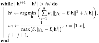
The weighted least squares can also be used with 1 -regularization. In practice, variance might not be known exactly. Moreover, the real noise may be non-Gaussian, and the observations may contain many outliers. In this case, the iteratively reweighted least squares (IRLS) method should be applied. Algorithm 1 outlines this method.
Inputs of the IRLS method are tolerance t o l needed to stop the search when improvements become negligible and a regularization parameter δ needed to avoid division by zero in points where the error | y k i E i h j | becomes zero. The parameter δ is used as the minimal absolute value of the denominator, and limits the highest value of w i with 1 / δ .
Algorithm 1: Iteratively reweighted least squares (IRLS) with 1 -regularization
Input: t o l , δ .
Output: h k .
Initialization:
w i 0 1 , i = [ 1 . . n ] ,
h 0 0 ,
j 0
Mathematics 09 02999 i001
h k h j .

2.2. Mechanical System Identification

Let a mechanical system state be described by a vector of coordinates x and a vector of velocities x ˙ . When the system is stationary and linear, the equation of dynamics is written as
M x ¨ + 2 C x ˙ + K x = f ( t ) ,
where M stands for a matrix of inertia, C stands for a damping matrix, K is a stiffness matrix, and f ( t ) is external driving force.
In many practical cases, matrices of inertia and damping are linear, but K depends on x ; therefore, we should investigate the following case:
M x ¨ + 2 C x ˙ + F ( x ) = f ( t ) .
A piece-wise linear F ( x ) can be described as
F ( x ) = K 1 ( x x 01 ) ( x X 1 ) , K 2 ( x x 02 ) ( x X 2 ) , K p ( x x 0 p ) ( x X p ) ,
where X j is a certain region in the phase space, K j is a matrix and x 0 j is a certain term.
Let a function μ j ( x ) return 1 if x X j , and 0 otherwise. The functions μ j may be obtained analytically or via support vector machine technique or logistic classification.
Then, the Equation (10) reads:
M x ¨ + 2 C x ˙ + i = j p K j μ j ( x ) ( x x 0 j ) = f ( t ) .
Let us write this equation as the first order ODE, assuming that M is non-degenerate:
x ˙ = v , v ˙ = 2 M 1 C v M 1 j = 1 p K j μ j ( x ) ( x x 0 j ) + M 1 f ( t ) .
Speaking of identification, the first equation in (13) is trivial, and the second can be treated as a special case of a general equation of dynamics. Suppose that the term g ( t ) = M 1 f ( t ) and the acceleration a = v ˙ are known. When we have n observations on the system state, we can use the identity
a i g ( t i ) y i = A v i + j = 1 p B j μ i ( x i ) ( x i x 0 j ) , i = [ 1 . . n ] ,
for reconstructing the unknown matrices A = 2 M 1 C and B j = M 1 K j via least squares from time series { a i } , { v i } , { x i } , { t i } .
When we have only time series for { a i } and { t i } and should reconstruct two others, we perform double integration due to relation
{ a i } { v i } { x i } .
This approach may cause some problems with state space reconstruction in practical applications:
1. Integration of noisy signal introduces a trend, which is challenging to eliminate, and the more integrations are performed, the more complicated problem is.
2. Integration of noisy signal tends to smooth the signal, masking high-speed, high-frequency processes with the noise, leading to decreasing the signal-to-noise ratio of these components in the entire signal.
The latter circumstance leads to underestimation of the matrices A and, especially, B j .
Proposition 1.
For practical purposes, in the case of a noisy signal, both sides of the Equation (14) may be differentiated, and unknown matrices may be found from the obtained relation more precisely.
The following relation is underlying the Proposition 1:
{ j i } d d t { a i } { v i } ,
where j denotes jerk. As stated by the Proposition 1, the Equation (14) turns into:
j i g ˙ ( t i ) y i = A a i + j = 1 p B j d d t μ j ( x i ) ( x i x 0 j ) , i = [ 1 . . n ] .
Derivative of μ j ( x ( t ) ) equals to:
d d t μ j ( x ( t ) ) = 0 , ( x X j ) , ± ( x B j ) ,
where B j denotes the border of X j . In practice, one may treat the probability of x i being on the border infinitesimally small, so (15) can be rewritten as
j i g ˙ ( t i ) y i = A a i + j = 1 p B j μ j ( x i ) v i , i = [ 1 . . n ] .
The relation (16) is further used for estimating A and B j . The following advantages over using (14) for identification can be achieved:
1. Only single integration and single differentiation are performed for obtaining independent variables, and double integration is needed for obtaining only values of μ j ( x ) . Therefore, numerical errors due to these operations are minimal.
2. High-frequency signal component suppression after integration and high-frequency noise amplification after differentiation are minimal.
These two advantages lead to more precise parameter estimation. Nevertheless, rigorous theoretical proof of the Proposition 1 meets sufficient difficulties since it involves several unknown parameters such as noise, parameters of motion, type of numerical method used for integration and differentiation, and parameters of numerical noise introduced by the computer. These circumstances force us to study the practical advantage of the proposed approach via numerical simulation and experiment.
Further, we utilize the abbreviation DIA (double integration approach) in relation to the Equation (14) and IDA (integrate-and-differentiate approach) in relation to the Equation (16).
Algorithm 2 outlines system identification via DIA.
Algorithm 2: DIA for parametric identification of piece-wise linear mechanical system
Input: { x i } , { v i } , { a i } , { t i }
Output: h .
Initialization:
1. Set incidence vectors
I j = μ j ( x 1 ) μ j ( x 2 ) μ j ( x n ) n × 1 , j = [ 1 . . p ] ,
2. Find
X = x 1 x 2 x n n × m , V = v 1 v 2 v n n × m , X 0 j = x 0 j x 0 j x 0 j n × m , j = [ 1 . . p ] ,
3. Calculate
E = V , I 1 ( X X 01 ) , I 2 ( X X 02 ) , I p ( X X 0 p ) n × m p ,
where ∘ denotes element-wise product,
4. y i = a i g ( t i ) .
Mathematics 09 02999 i002
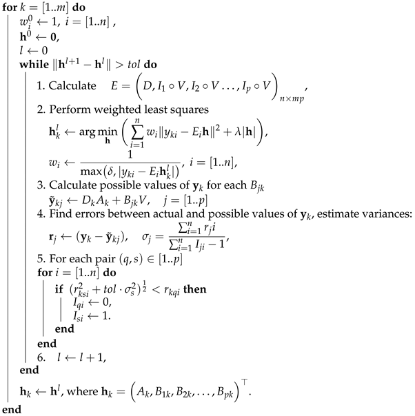
The IDA is described with Algorithm 3. It is rather similar to Algorithm 2 with another definition of the matrix E and using the modification of the IRLS: IRLS with swapping. The motivation and description of this modification are as follows.
Algorithm 3: IDA for parametric identification of piece-wise linear mechanical system
Input: { x i } , { v i } , { a i } , { j i } , { t i }
Output: h .
Initialization:
1. Set incidence vectors
I j = μ j ( x 1 ) μ j ( x 2 ) μ j ( x n ) n × 1 , j = [ 1 . . p ] ,
2. Find
D = a 1 a 2 a n n × m , V = v 1 v 2 v n n × m ,
3. y i = j i g ˙ ( t i ) .
Mathematics 09 02999 i003
In a realistic scenario, there is some significant errors in x i , so that the values of μ j ( x i ) are incorrect in some cases; thus, the vectors I j are determined with errors. In order to correct this error, we include a swapping step needed to correspond the vectors v i multiplied by I j to correct stiffness matrices B j .
Suppose, it was determined initially that x i X q , but the particular value y i k is better predicted if x i X s . Then, we should swap the values in the incidence vectors:
I q i 0 , I s i 1 .
Suppose σ s 2 is the variance of prediction when x i X s . Let r k q i 2 be the squared error of estimating y k i obtained when x i X q and let r k s i 2 be the squared error of estimating y k i obtained when x i X s . To avoid overtraining of the model, we must perform swapping only if
r k s i 2 + t o l · σ s 2 < r k q i ,
where t o l is the tolerance parameter.
The IRLS with swapping is outlined in Algorithm 3 in detail.
The proposed approach can be applied to the general form of the mechanical system, which equation after differentiating of (10) reads:
M x ( 3 ) + 2 C x ¨ + K ( x ) x x ˙ ( x x 0 j ) + K ( x ) x ˙ = f ˙ ( t ) .
Nevertheless, the special case of K ( x ) written as (11) is very common and makes the problem formulation easier, so we focused on it directly.

3. Study of Chaotic Mechanical System with Backlash

3.1. Lin-Ewins Mechanical Oscillator

Chaotic vibration in mechanical constructions has gained special attention since the early 1990s, when several simple chaotic systems have been discovered, including a double pendulum [34] and an oscillator with backlash [35], based on the Duffing equation. The latter work is of particular interest since it introduces a system described by the equation of type (10). In this work, R. Lin and D. Ewins proposed a nonlinear mechanical system with backlash, which is shown in Figure 1.
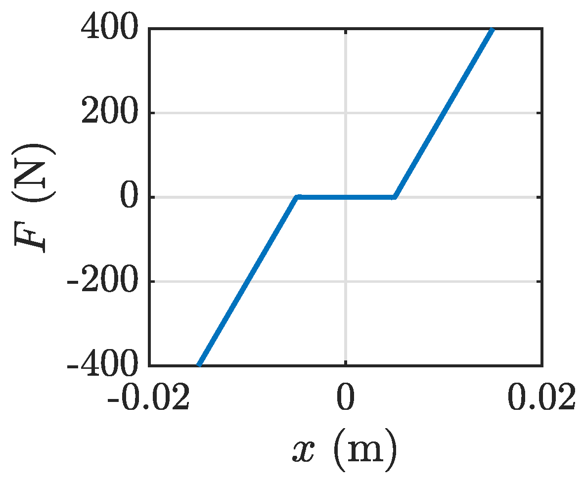
The system consists of a mass m suspended between two symmetric springs with stiffness k 1 and dampers with damping coefficients equal to c. There are two additional springs with stiffness k 2 k 1 with a backlash x 0 between the mass and the springs. The overall force caused by springs for the parameter values x 0 = 5 · 10 3 m, k 2 = 40 , 000 N/m and k 1 = 0 N/m is shown in Figure 2, corresponding to the case when there are only two springs with backlash.
The equation of motion of this mechanical system excited by a sinusoidal force is as follows:
m x ¨ + 2 c x ˙ + F ( x ) = A cos ω t ,
where F ( x ) is a piece-wise linear function:
F ( x ) = k 2 μ 1 ( x ) ( x + x 0 ) + k 1 μ 2 ( x ) x + k 2 μ 3 ( x ) ( x x 0 ) ,
where
μ 1 ( x ) = 1 ( x x 0 ) 0 ( x > x 0 ) μ 3 ( x ) = 1 ( x x 0 ) 0 ( x < x 0 ) , μ 2 ( x ) = 1 μ 1 ( x ) μ 3 ( x ) .
The direct application of Equation (20) may cause malfunction of some ODE solvers because of discontinuous functions. In order to avoid inaccuracies during numerical simulation, we used the following sigmoidal approximations of μ 1 ( x ) and μ 3 ( x ) :
μ 1 ( x ) = 1 1 + e s ( x x 0 ) , μ 3 ( x ) = 1 1 + e s ( x x 0 ) ,
where s = 10 4 is the parameter controlling the slope of the sigmoid near x 0 and x 0 .
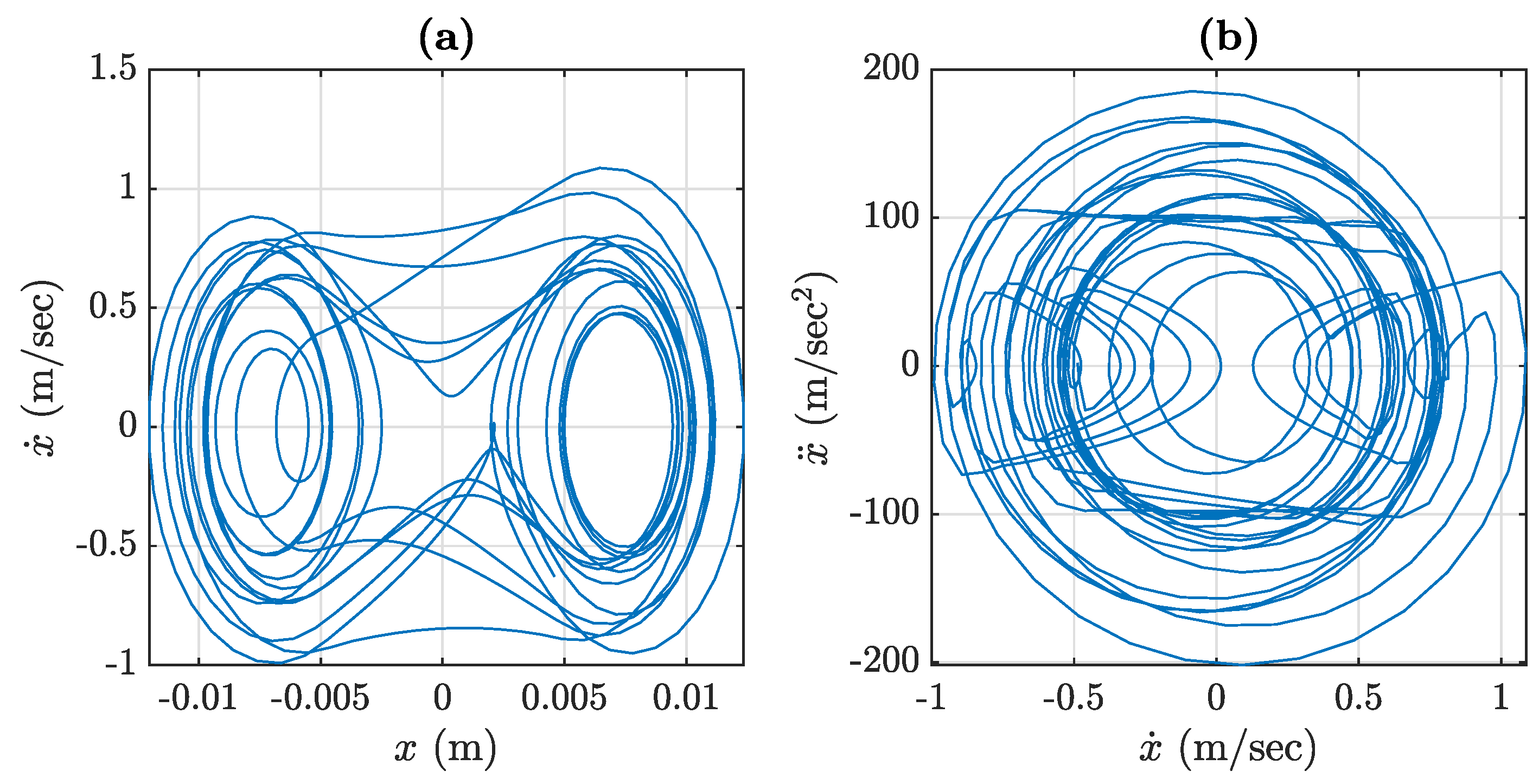
The following parameters of the system were used for the study: c = 4 N · s/m, x 0 = 5 · 10 3 m, k 2 = 40 , 000 N/m, k 1 = 0 N/m, A = 100 N, m = 1 kg, ω = 40 rad/s. We use ode45 MATLAB solver with x ( 0 ) = ( 0 , 0 ) , and a constant stepsize h = 10 3 s. With these parameters, the system demonstrates a chaotic behavior, as shown in Figure 3.
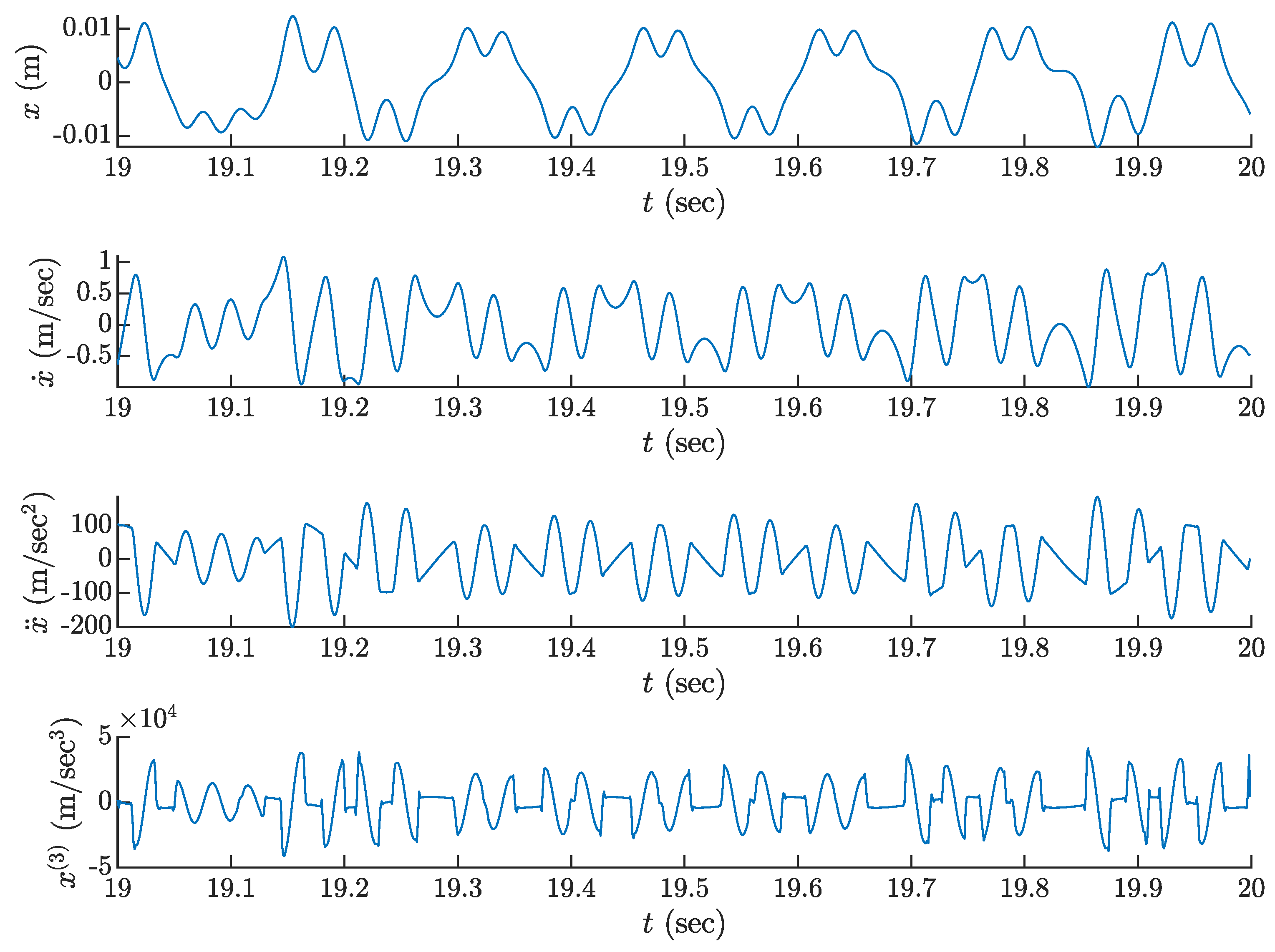
Figure 4 presents time series for successive derivatives of the displacement x up to the jerk x ( 3 ) .
Rewrite the system (18) in a form of the first-order ODE:
x ˙ = v , v ˙ = 2 c v m F ( x ) m + A m cos ( ω t ) .
The second equation of the system (22) can be used for the system identification.

3.2. Identification of Nonlinear Stiffness in Lin-Ewins Oscillator

Let the accelerometer be mounted on a mass m, and its signal { a i } is sampled over time series { t i } . Let the driving force A cos ( ω t ) be known exactly, as well as the mass m and damping coefficient c, and the series for speed { v i } and displacement { x i } are obtained by integration. Rewrite the second equation of (22) in a form appropriate for parametric identification via least squares, corresponding to DIA:
a i + 2 c v i m A m cos ( ω t i ) y i = F ( x i ) m .
Differentiating both sides of this equation, one can obtain a form appropriate for parametric identification via least squares, corresponding to IDA:
j i + 2 c a i m + A ω m sin ( ω t i ) y i = G ( x i ) m ,
where the series for jerk { j i } can be obtained by differentiation, and 
G ( x i ) = k 2 μ 1 ( x i ) v i + k 1 μ 2 ( x i ) v i + k 2 μ 3 ( x i ) v i .
We perform the comparison of identification approaches in two situations. First, we assume there is no noise in the time series for { a i } , and then, we add a Gaussian noise showing that in both cases, the IDA performs better than DIA.

3.2.1. Noiseless Case

To implement the identification via DIA, we twice integrate time series of { a i } for obtaining { v i } and { x i } and then perform Algorithm 2.
For identification via IDA we integrate time series of { a i } for obtaining { v i } and { x i } and differentiate it for obtaining { j i } and then perform Algorithm 3. The simulation included 2 · 10 4 points corresponding to 20 s of simulation with sampling frequency f = 1 kHz.
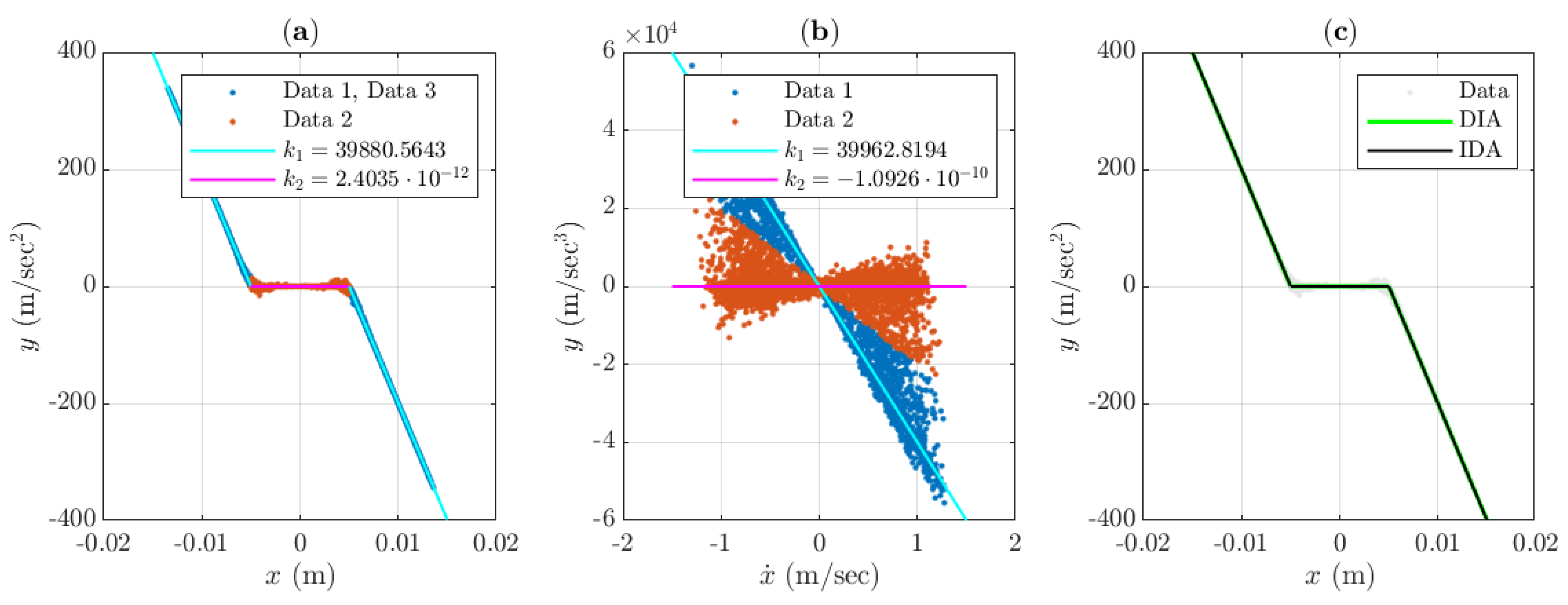
The comparison of system identification approaches is given in Figure 5.

3.2.2. Case of Additive Gaussian Noise

Accelerometer typical errors include the presence of additive white Gaussian noise and zero point drift, which is especially inherent to widely spread piezoelectric accelerometers [36]. These errors can be modeled with the following equation:
a i = a ( t i ) + σ z i + a 0 ,
where a i is the sample obtained from the accelerometer, a ( t i ) is the true acceleration, z i is a standard normal random variable, σ is standard deviation and a 0 is zero point drift. In our experiment, we set the following values: σ = 10 m/s 2 , a 0 = 5 m/s 2 , which is about 5% and 2.5% of the acceleration amplitude, respectively. In order to eliminate possible trends in { v i } and { x i } we split the time series into 20 fragments and integrate them independently from zero and then filter them with an ideal notch filter with band 0–2 Hz, and then eliminate linear trends.
The comparison of system identification approaches is given in Figure 6. It is clearly seen that the DIA failed to find the value of k 1 with enough accuracy, while the IDA performed rather well. The overall results are given in Table 1.
The relative error in Table 1 was calculated as
r e l e r r = k ^ 1 k 1 k 1 ,
where k ^ 1 is the estimated value of k 1 with its actual value k 1 = 40 , 000 .
In all cases, k 1 was found much more accurate via IDA, and the error of estimation of k 2 was below the accepted numerical error.

4. Experimental Study of Nonlinear Vibration of an Aluminum Beam

Aluminum extruded profile is often used for building frames, racks, enclosures in many industrial applications. It has a large variety of shapes and allows creating sophisticated constructions using various connection elements. A majority of profile manufacturers follow Bosh Rexroth standard [37] and therefore are compatible with each other. In our study, we investigate free vibrations of a vertical 20 × 20 mm beam made of aluminum profile mounted on a 20 × 40 mm fixed aluminum profile with one L-shape inner bracket made of silumin. This joint has sufficiently different stiffness for positive and negative beam tilt direction due to different stress distribution in detail. Figure 7 shows the experimental setup and its schematics.
The equation of motion of this mechanical system is as follows:
J θ ¨ + σ θ ˙ + F ( θ ) = 0 ,
where σ = 2 c is a total damping coefficient and F ( θ ) is a piece-wise linear function:
F ( θ ) = k 1 μ 1 ( θ ) θ + k 2 μ 2 ( θ ) θ ,
where
μ 1 ( θ ) = 1 ( θ 0 ) 0 ( θ < 0 ) , μ 2 ( θ ) = 1 ( θ > 0 ) 0 ( θ 0 ) .
The parameters of the setup were as follows: beam length L = 0.38 m, mass of the accelerometer with a mounting clamp m 1 = 0.05 kg, distance between top of the beam and the accelerometer h = 0.01 m, mass of the beam m 2 = 0.160 kg, from where the center of inertia is estimated as
L c = ( m 1 ( L h ) + m 2 L / 2 ) / ( m 1 + m 2 ) = 0.2329   m ,
and moment of inertia is
J = ( m 1 + m 2 ) L c 2 = 1.139 · 10 2 kg · m 2 .
The linear damping parameter of the system can be easily found from the rate of vibration amplitude decay over time and was estimated as σ = 0.045 N · sec/rad. Stiffness identification is much more challenging.
The system (25) in a form appropriate for stiffness identification via DIA reads:
θ ¨ + σ J θ ˙ y = k 1 J μ 1 ( θ ) θ k 2 J μ 2 ( θ ) θ .
Identification via IDA uses the following equation:
θ ( 3 ) + σ J θ ¨ y = k 1 J μ 1 ( θ ) θ ˙ k 2 J μ 2 ( θ ) θ ˙ .
In our study, we used IMV VP-4200 piezoelectric accelerometer connected to NI PXI system for data acquisition. The sampling frequency was 1000 Hz. We recorded 10 time series up to 1 s length, thus obtaining 5375 points of data. We used the differentiation method of order 4 based on central differences and the integration method of accuracy order 3 based on Simpson’s rule for obtaining a derivative and integrals of the acceleration. The following relation was used for calculating angular acceleration from linear one:
θ ¨ = x ¨ L ,
where x ¨ is linear acceleration measured with the accelerometer.
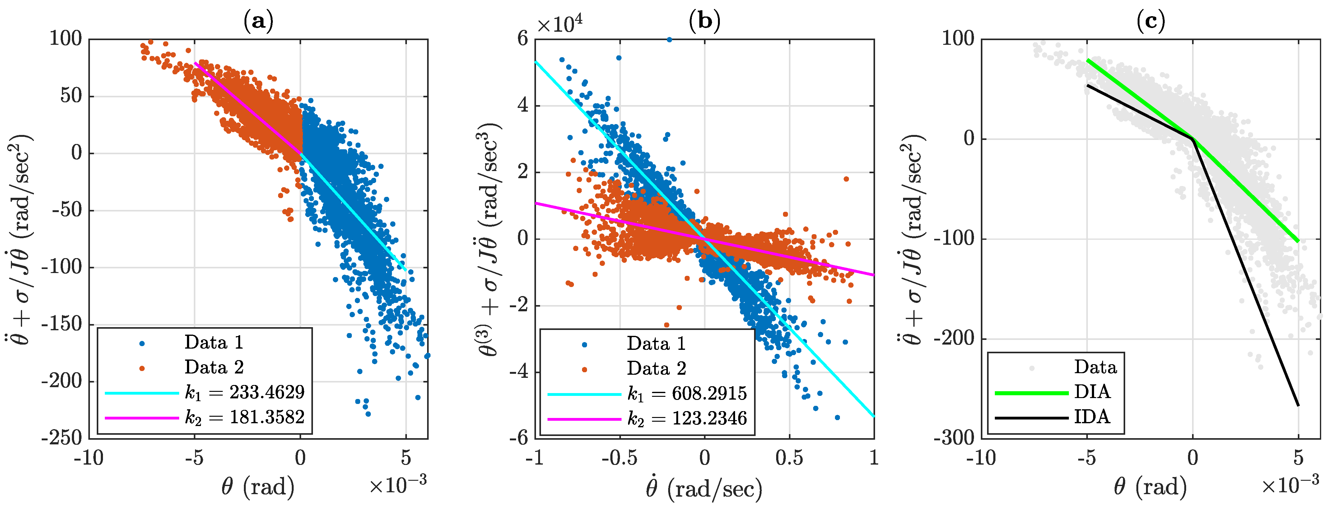
The results of stiffness identification are shown in Figure 8. The obtained values for k 1 and k 2 are summarized in Table 2.
One can see that in comparison to IDA, DIA underestimates k 1 and overestimated k 2 , which corresponds to dynamics closer to harmonic oscillations rather than nonlinear behavior.
The time domain signals for the tilt angle θ shown in Figure 9. This simulation was performed by ode45 MATLAB solver with fixed stepsize h = 10 3 s.
In our simulations, we used the sigmoidal approximations similar to (21) for μ 1 ( θ ) and μ 2 ( θ ) to avoid inaccuracies caused by discontinuities in F ( θ ) :
μ 1 ( θ ) = 1 1 + e s θ , μ 2 ( θ ) = 1 1 + e s θ ,
where s = 10 4 .
From Figure 9, the advantage of IDA over DIA is obvious, especially in reconstructing third angle derivative θ ( 3 ) , where the shape is reproduced in the model obtained via IDA rather realistically, unlike in the model obtained via DIA.
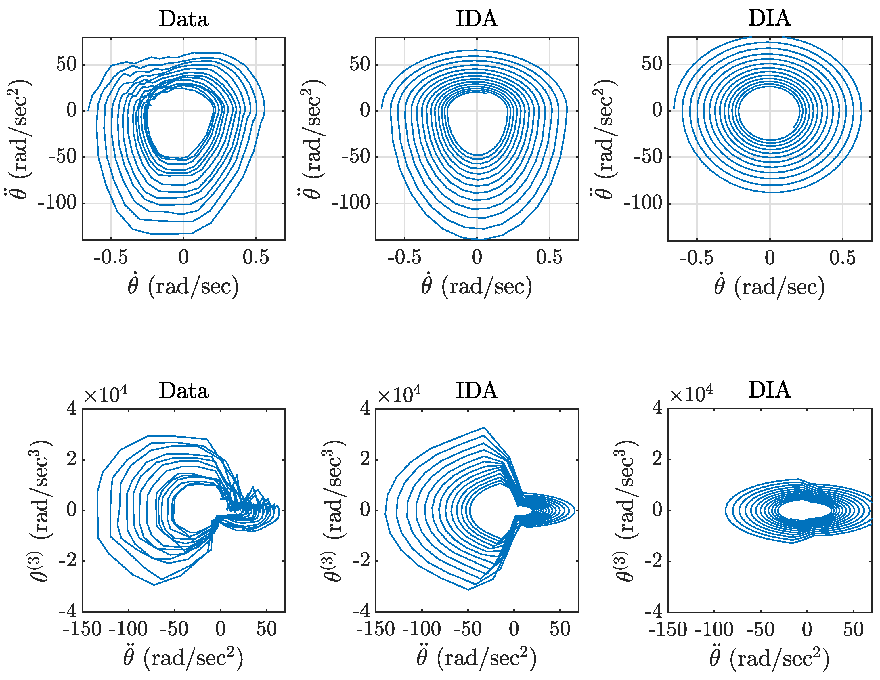
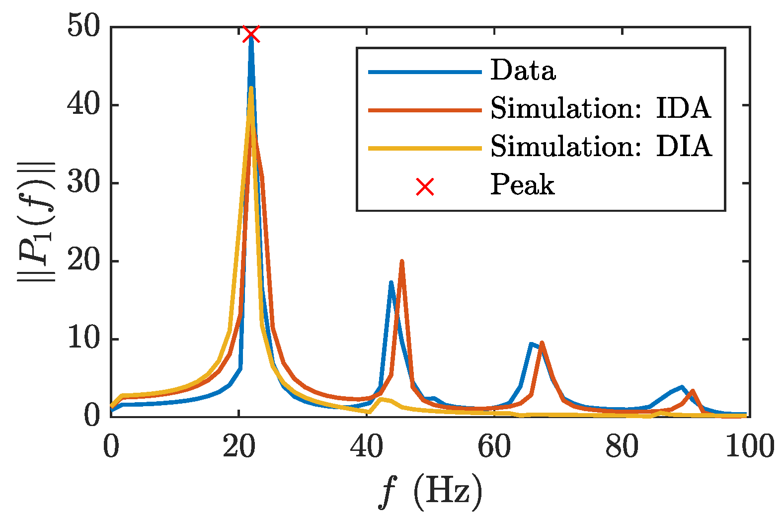
One can clearly see that there is a notable advantage of IDA over DIA in Figure 10. While some specific features are not reproduced in the model, such as a slight asymmetry of a trajectory shape (compare the left column with two others), the overall shape is reconstructed much more accurate with IDA than with DIA. Comparison of power spectra of acceleration signal obtained in experiment and simulations in models identified with IDA and DIA is given in Figure 11.
From Figure 11, it is also clearly seen that while both approaches allow reproducing the first harmonic rather precisely, the other harmonics are almost absent in the signal from the model identified with DIA.

5. Conclusions and Discussion

In this study, we considered the problem of nonlinear mechanical system identification in the form of piece-wise linear ODE from accelerometer data using a variant of the iteratively reweighted least squares method. Two aspects of the identification process were highlighted in detail.
First, we demonstrated by simulation and experimental means that using noisy acceleration series may sufficiently decrease the accuracy of the parameter identification. Thus, we propose using a differentiated governing equation containing acceleration and velocity as independent variables, and position as an auxiliary variable needed for data classification. We call an approach based on the conventional governing equation in velocity and position a double integration approach (DIA), and the proposed approach is called the integrate-and-differentiate approach (IDA).
Second, we proposed a modification of the iteratively reweighted least squares method for using with IDA. Our modification includes an auxiliary reclassification step, and the modified method is called iteratively reweighted least squares with swapping. Applying this method allows improving identification accuracy through eliminating errors in classification needed for parameter estimation of piece-wise linear ODEs.
There is a number of practical applications of the proposed approach. Accurate mathematical models given as differential equations are needed in various scientific and engineering areas, having many advantages over the other models. Special attention is paid to them in applications of nonlinear science. For instance, electronic chaotic system design and investigation require high-precision modeling, for which parameter identification can be performed [38,39]. Digital chaotic systems are often used for data encryption, and system identification can be used for a cryptographic attack against a chaotic encryption method [40]. Recent experimental studies of chaos in mechanics confirmed theoretical predictions made several decades ago. For example, a chaotic system resembling the Lin-Ewins oscillator was investigated by R.J. Chang and Y.-C. Wang in 2020 [41]. These are only a few illustrations of why system identification, and particularly, the identification of mechanical systems from accelerometer data, is of great importance.

Author Contributions

Conceptualization, A.I.K. and D.B.; data curation, E.K. and D.B.; formal analysis, E.K. and E.G.N.; investigation, A.I.K. and E.K.; methodology, A.I.K.; project administration, D.B. and E.G.N.; resources, E.G.N.; software, A.I.K. and E.K.; supervision, A.I.K. and D.B.; validation, D.B.; visualization, E.K.; writing—original draft, A.I.K.; writing—review and editing, D.B. and E.G.N. All authors have read and agreed to the published version of the manuscript.

Funding

This research received no external funding.

Institutional Review Board Statement

Not applicable.

Informed Consent Statement

Not applicable.

Conflicts of Interest

The authors declare no conflict of interest.

Abbreviations

The following abbreviations are used in this manuscript:
ODEOrdinary Differential Equation
OLSOrdinary Least Squares
IRLSIteratively Reweighted Least Squares
DIADouble Integration Approach
IDAIntegrate-and-Differentiate Approach

References

  1. Kera, H.; Hasegawa, Y. Noise-tolerant algebraic method for reconstruction of nonlinear dynamical systems. Nonlinear Dyn. 2016, 85, 675–692. [Google Scholar] [CrossRef]
  2. Obeid, S.; Ahmadi, G.; Jha, R. NARMAX Identification Based Closed-Loop Control of Flow Separation over NACA 0015 Airfoil. Fluids 2020, 5, 100. [Google Scholar] [CrossRef]
  3. Tian, R.; Yang, Y.; van der Helm, F.C.; Dewald, J. A novel approach for modeling neural responses to joint perturbations using the NARMAX method and a hierarchical neural network. Front. Comput. Neurosci. 2018, 12, 96. [Google Scholar] [CrossRef] [Green Version]
  4. Brusaferri, A.; Matteucci, M.; Portolani, P.; Spinelli, S. Nonlinear system identification using a recurrent network in a Bayesian framework. In Proceedings of the 2019 IEEE 17th International Conference on Industrial Informatics, Helsinki-Espoo, Finland, 22–25 July 2019; Volume 1, pp. 319–324. [Google Scholar]
  5. Yang, L.; Liu, J.; Yan, R.; Chen, X. Spline adaptive filter with arctangent-momentum strategy for nonlinear system identification. Signal Process. 2019, 164, 99–109. [Google Scholar] [CrossRef]
  6. Gedon, D.; Wahlström, N.; Schön, T.B.; Ljung, L. Deep state space models for nonlinear system identification. IFAC-PapersOnLine 2021, 54, 481–486. [Google Scholar] [CrossRef]
  7. Karimshoushtari, M.; Novara, C. Design of experiments for nonlinear system identification: A set membership approach. Automatica 2020, 119, 109036. [Google Scholar] [CrossRef]
  8. Davila, J.; Fridman, L.; Poznyak, A. Observation and Identification of Mechanical Systems via Second Order Sliding Modes. Int. J. Control 2006, 79, 232–237. [Google Scholar] [CrossRef] [Green Version]
  9. Kok, M.; Hol, J.D.; Schön, T.B. Using Inertial Sensors for Position and Orientation Estimation. Found. Trends Signal Process. 2017, 11, 1–153. [Google Scholar] [CrossRef] [Green Version]
  10. Karimov, A.; Nepomuceno, E.G.; Tutueva, A.; Butusov, D. Algebraic method for the reconstruction of partially observed nonlinear systems using differential and integral embedding. Mathematics 2020, 8, 300. [Google Scholar] [CrossRef] [Green Version]
  11. Singh, A.; Moore, K.J. Characteristic nonlinear system identification of local attachments with clearance nonlinearities. Nonlinear Dyn. 2020, 102, 1667–1684. [Google Scholar] [CrossRef]
  12. Pham, M.T.; Gautier, M.; Poignet, P. Accelerometer based identification of mechanical systems. In Proceedings of the 2002 IEEE International Conference on Robotics and Automation, Washington, DC, USA, 11–15 May 2002; Volume 4, pp. 4293–4298. [Google Scholar]
  13. Ewald, V.; Venkat, R.S.; Asokkumar, A.; Benedictus, R.; Boller, C.; Groves, R.M. Perception modelling by invariant representation of deep learning for automated structural diagnostic in aircraft maintenance: A study case using DeepSHM. Mech. Syst. Signal Process. 2021, 165, 108153. [Google Scholar] [CrossRef]
  14. Peng, G.C.; Alber, M.; Tepole, A.B.; Cannon, W.R.; De, S.; Dura-Bernal, S.; Garikipati, K.; Karniadakis, G.; Lytton, W.W.; Perdikaris, P.; et al. Multiscale modeling meets machine learning: What can we learn? Arch. Comput. Methods Eng. 2021, 28, 1017–1037. [Google Scholar] [CrossRef] [Green Version]
  15. Hanke, S.; Peitz, S.; Wallscheid, O.; Böcker, J.; Dellnitz, M. Finite-control-set model predictive control for a permanent magnet synchronous motor application with online least squares system identification. In Proceedings of the 2019 IEEE International Symposium on Predictive Control of Electrical Drives and Power Electronics, Quanzhou, China, 31 May–2 June 2019; pp. 1–6. [Google Scholar]
  16. Galrinho, M. Least Squares Methods for System Identification of Structured Models. Ph.D. Thesis, KTH Royal Institute of Technology, Stockholm, Sweden, 2016. [Google Scholar]
  17. Elisei-Iliescu, C.; Paleologu, C.; Benesty, J.; Stanciu, C.; Anghel, C.; Ciochină, S. Recursive least-squares algorithms for the identification of low-rank systems. IEEE/ACM Trans. Audio Speech Lang. Process. 2019, 27, 903–918. [Google Scholar] [CrossRef]
  18. Tierney, C.; Mulgrew, B. Adaptive waveform design with least-squares system identification for interference mitigation in SAR. In Proceedings of the 2017 IEEE Radar Conference (RadarConf), Seattle, WA, USA, 8–12 May 2017; pp. 180–185. [Google Scholar]
  19. Xia, B.; Zhao, X.; De Callafon, R.; Garnier, H.; Nguyen, T.; Mi, C. Accurate Lithium-ion battery parameter estimation with continuous-time system identification methods. Appl. Energy 2016, 179, 426–436. [Google Scholar] [CrossRef] [Green Version]
  20. Ljung, L. Consistency of the least-squares identification method. IEEE Trans. Autom. Control 1976, 21, 779–781. [Google Scholar] [CrossRef]
  21. Manikantan, R.; Chakraborty, S.; Uchida, T.K.; Vyasarayani, C. Parameter identification in nonlinear mechanical systems with noisy partial state measurement using PID-controller penalty functions. Mathematics 2020, 8, 1084. [Google Scholar] [CrossRef]
  22. Bian, Q.; Zhao, K.; Wang, X.; Xie, R. System identification method for small unmanned helicopter based on improved particle swarm optimization. J. Bionic Eng. 2016, 13, 504–514. [Google Scholar] [CrossRef]
  23. Cortez-Vega, R.; Maldonado, J.; Garrido, R. Parameter Identification using PSO under measurement noise conditions. In Proceedings of the 2019 6th International Conference on Control, Decision and Information Technologies, Le Cnam, Paris, 23–26 April 2019; pp. 103–108. [Google Scholar]
  24. Kommenda, M.; Burlacu, B.; Kronberger, G.; Affenzeller, M. Parameter identification for symbolic regression using nonlinear least squares. Genet. Program. Evolvable Mach. 2020, 21, 471–501. [Google Scholar] [CrossRef] [Green Version]
  25. Brunton, S.L.; Proctor, J.L.; Kutz, J.N. Discovering governing equations from data by sparse identification of nonlinear dynamical systems. Proc. Natl. Acad. Sci. USA 2016, 113, 3932–3937. [Google Scholar] [CrossRef] [Green Version]
  26. Mateos, G.; Giannakis, G.B. Robust nonparametric regression via sparsity control with application to load curve data cleansing. IEEE Trans. Signal Process. 2011, 60, 1571–1584. [Google Scholar] [CrossRef] [Green Version]
  27. Daubechies, I.; DeVore, R.; Fornasier, M.; Güntürk, C.S. Iteratively reweighted least squares minimization for sparse recovery. Commun. Pure Appl. Math. A J. Issued Courant Inst. Math. Sci. 2010, 63, 1–38. [Google Scholar] [CrossRef] [Green Version]
  28. Kümmerle, C.; Mayrink Verdun, C.; Stöger, D. Iteratively Reweighted Least Squares for 1-minimization with Global Linear Convergence Rate. arXiv 2020, arXiv:2012.12250. [Google Scholar]
  29. Xie, L.; Zhou, Z.; Zhao, L.; Wan, C.; Tang, H.; Xue, S. Parameter identification for structural health monitoring with extended Kalman filter considering integration and noise effect. Appl. Sci. 2018, 8, 2480. [Google Scholar] [CrossRef] [Green Version]
  30. Huang, G.P.; Mourikis, A.I.; Roumeliotis, S.I. Analysis and improvement of the consistency of extended Kalman filter based SLAM. In Proceedings of the 2008 IEEE International Conference on Robotics and Automation, Pasadena, CA, USA, 22–25 May 2008; pp. 473–479. [Google Scholar]
  31. Nordin, M.; Gutman, P.O. Controlling mechanical systems with backlash—A survey. Automatica 2002, 38, 1633–1649. [Google Scholar] [CrossRef]
  32. Yao, H.; Cao, Y.; Zhang, S.; Wen, B. A novel energy sink with piecewise linear stiffness. Nonlinear Dyn. 2018, 94, 2265–2275. [Google Scholar] [CrossRef] [Green Version]
  33. Wang, Y. Dynamics of unsymmetric piecewise-linear/non-linear systems using finite elements in time. J. Sound Vib. 1995, 185, 155–170. [Google Scholar] [CrossRef] [Green Version]
  34. Levien, R.; Tan, S. Double pendulum: An experiment in chaos. Am. J. Phys. 1993, 61, 1038–1044. [Google Scholar] [CrossRef]
  35. Lin, R.; Ewins, D. Chaotic vibration of mechanical systems with backlash. Mech. Syst. Signal Process. 1993, 7, 257–272. [Google Scholar] [CrossRef]
  36. Korobiichuk, I. Analysis of Errors of Piezoelectric Sensors used in Weapon Stabilizers. Metrol. Meas. Syst. 2017, 24, 91–100. [Google Scholar] [CrossRef]
  37. Bosch Rexroth. Basic Mechanic Elements. Available online: https://www.boschrexroth.com/en/xc/products/product-groups/assembly-technology/basic-mechanic-elements (accessed on 8 September 2021).
  38. Karimov, T.; Butusov, D.; Andreev, V.; Karimov, A.; Tutueva, A. Accurate synchronization of digital and analog chaotic systems by parameters re-identification. Electronics 2018, 7, 123. [Google Scholar] [CrossRef] [Green Version]
  39. Karimov, A.; Tutueva, A.; Karimov, T.; Druzhina, O.; Butusov, D. Adaptive generalized synchronization between circuit and computer implementations of the Rössler system. Appl. Sci. 2021, 11, 81. [Google Scholar] [CrossRef]
  40. Tutueva, A.V.; Nepomuceno, E.G.; Karimov, A.I.; Andreev, V.S.; Butusov, D.N. Adaptive chaotic maps and their application to pseudo-random numbers generation. Chaos Solitons Fractals 2020, 133, 109615. [Google Scholar] [CrossRef]
  41. Chang, R.J.; Wang, Y.C. Experimental Investigation on the Lumped Model of Nonlinear Rocker–Rocker Mechanism with Flexible Coupler. J. Dyn. Syst. Meas. Control 2020, 142, 061004. [Google Scholar] [CrossRef]
Figure 1. Chaotic mechanical system with backlash. The following parameters of the system were proposed by R. Lin and D. Ewins resulting in a chaotic behavior of the system under periodic excitation: c = 4 N · s/m, x 0 = 5 · 10 3 m, k 2 = 40 , 000 N/m, k 1 = 0 N/m.
Mathematics 09 02999 g001
Figure 2. Nonlinear force-displacement dependency.
Mathematics 09 02999 g002
Figure 3. Phase space of the Lin-Ewins chaotic system: (a) the x- x ˙ phase space projection; (b) x ˙ - x ¨ phase space projection.
Mathematics 09 02999 g003
Figure 4. Time series for the Lin-Ewins chaotic system.
Mathematics 09 02999 g004
Figure 5. Results of the Lin-Ewin system identification with DIA and IDA: (a) data are divided into three subsets Data 1, Data 2, and Data 3 containing x i corresponding to μ i ( x i ) = 1 . The subsets Data 1 and Data 3 are colored blue; Data 2 is colored red; (b) data are divided into two subsets Data 1 corresponding to μ 1 ( x i ) = 1 or μ 3 ( x i ) = 1 , and Data 2 corresponding to μ 2 ( x i ) = 1 . Both results are shown in the panel (c) and look rather similar, while the accuracy of finding k 1 is slightly better in case of IDA, and k 2 in both cases is very close to zero.
Mathematics 09 02999 g005
Figure 6. Results of the Lin-Ewin system identification with DIA and IDA with additive Gaussian noise. The legend is similar to Figure 5: (a) DIA; (b) IDA; both results are shown in (c). DIA failed in estimating k 1 and IDA was still fruitful, while k 2 in both cases was estimated properly.
Mathematics 09 02999 g006
Figure 7. Panel (a) shows a photo of an experimental setup, panel (b) shows a drawing of the setup, where 1 is a vertical vibrating beam, 2 is an inner bracket and 3 is an accelerometer. Panel (c) shows the system schematics. The denoted angle in the panel corresponds to a positive direction of the beam tilt.
Mathematics 09 02999 g007
Figure 8. Results of the nonlinear beam identification with DIA and IDA. In both cases, Data 1 corresponds to negative tilt angle θ , Data 2 corresponds to positive tilt angle θ . Panel (a) illustrates results of DIA, panel (b) illustrates results of IDA, both results are shown in the panel (c). Being compared with IDA, DIA underestimates k 1 and overestimated k 2 , which corresponds to dynamics closer to harmonic oscillations rather then nonlinear ones.
Mathematics 09 02999 g008
Figure 9. Fragment of time-domain signals representing various derivatives of angular displacement θ with comparison between real signals and two models obtained with the described identification approaches.
Mathematics 09 02999 g009
Figure 10. Phase space of nonlinear beam in two planes: θ ˙ - θ ¨ and θ ¨ - θ ( 3 ) .
Mathematics 09 02999 g010
Figure 11. Power spectra of the measured signal (blue) and simulated signals in models obtained via IDA (red) and DIA (yellow).
Mathematics 09 02999 g011
Table 1. Comparison of stiffness identification in the Lin-Ewins system.
ApproachEstimated k 1 Relative Error of k 1 Estimated k 2
DIA, without noise39,880.60.0030 2.4 · 10 12
IDA, without noise39,962.30.0009 1.1 · 10 10
DIA, with noise5963.90.85 5.5 · 10 12
IDA, with noise37,952.60.05 4.3 · 10 10
Table 2. Comparison of stiffness identification in the vibrating beam.
ApproachEstimated k 1 Estimated k 2
DIA233.5181.6
IDA608.3123.2
Publisher’s Note: MDPI stays neutral with regard to jurisdictional claims in published maps and institutional affiliations.