Shearing Effects on the Phase Coarsening of Binary Mixtures Using the Active Model B

Abstract

The phase separation of a two-dimensional active binary mixture is studied under the action of an applied shear through numerical simulations. It is highlighted how the strength of the external flow modifies the initial shape of growing domains. The activity is responsible for the formation of isolated droplets which affect both the coarsening dynamics and the morphology of the system. The characteristic dimensions of domains along the flow and the shear direction are modulated in time by oscillations whose amplitudes are reduced when the activity increases. This induces a broadening of the distribution functions of domain lengths with respect to the passive case due to the presence of dispersed droplets of different sizes.

1. Introduction

Over the last decades much research has been dedicated to studying active materials, i.e., non-equilibrium systems in which internal units continuously consume energy, usually stored in the environment, to self-propel [1,2,3,4,5]. Examples of active matter range from bacterial and algal suspensions [6,7,8,9] to colloidal particles acquiring motion through chemical reactions [10,11,12], up to the cytoskeleton of living cells [13,14,15], to name but a few. Importantly, to convert their energy into motion, particles violate time-reversal symmetry (TRS) at the micro-scale.

An active process of particular relevance to us is the motility-induced phase separation (MIPS), where a suspension of repulsive motile particles can phase separate into bulk dense (liquid) and dilute (vapor) regions [16,17,18]. This essentially occurs because active particles aggregate where they move slowly, thus leading to a local density increase causing a slowing down and further accumulation. The resulting clusters show highly dynamical particle exchange leading to macroscopic phase separation [19,20,21]. The kinetics of MIPS has been found to share many features with that of passive systems with attractive interactions, thus suggesting that TRS could be restored at the macroscale level [16,17,22,23,24,25,26,27]. However, large scale simulations of active Brownian particles [20,21,28,29] as well as experiments [10,11,12] reveal that MIPS may also exhibit further non-equilibrium features, such as the formation of mesoscopic vapor bubbles within the particles aggregates and microphase separation [20,28,29,30]. This scenario would indeed support the view that time-reversal symmetry is manifestly broken macroscopically.

Alongside particle-based simulations, the phenomenology of MIPS can be also described using continuum field theories, either by an explicit coarse-graining of the microscopic dynamics or via symmetry arguments and conservation laws [31]. The latter strategy has led to the construction of the Active Model B (AMB) [24,28,32], a field theory that, in the absence of solvent, essentially extends the passive model B [33] by incorporating an active gradient term that cannot be obtained from a free-energy functional, thus breaking time-reversal symmetry. The passive Model B (MB) falls within a class of phase-field models describing the kinetics of phase separation through a conserved scalar order parameter $\varphi$ capturing, for example, the density of colloids or the concentration in a binary mixture. If hydrodynamics can be neglected, the evolution of $\varphi$ is governed by a Cahn-Hilliard equation [34,35], where the thermodynamic force driving the relaxation of $\varphi$ stems from the functional derivative of a ${\varphi }^4$ free energy with square gradient terms. Such simplified description captures, for example, the result $R\sim t^{\alpha }$, for the dependence of the domain size R on time t with a characteristic growth exponent $\alpha =1/3$ [36].

MB provides a robust framework to describe the passive phase separation subject to an external shearing [37,38,39,40,41,42,43]. In that case the growth is anisotropic, being characterized by domains stretched and tilted along the flow direction as observed in simulations [42,44] and experiments [45]. Indeed, numerical solutions of the dynamical equation with shear [42] confirm the presence of anisotropy of growing domains, which are found to exhibit two typical lengths. Theoretical calculations based on a renormalization group analysis shows that the growth exponent ${\alpha }_y$ in the shear direction, perpendicular to the flow, is not changed by the applied velocity profile, while the exponent ${\alpha }_x$ along the flow direction is increased by 1 [41]. Moreover, relevant physical quantities are found to oscillate on a logarithmic time scale, due to a periodic stretching and breaking-up of domains. The interest towards the role of shear in phase ordering is still vivid, as witnessed by recent studies [46,47].

In the context of active matter, while efforts have been addressed to investigate the active phase separation in the absence of an external driving [20,21,28,48,49], much less is known about the dynamic response observed when a shear flow is applied. Though it was shown [50] that in AMB the transition from homogeneous to bulk phase separation belongs to the same universality class of equilibrium MB, numerical studies of coarsening in AMB provide different scenarios. In Refs. [32,51], for example, it was argued that in AMB without shear the size of growing domains is still compatible with a growth exponent $\alpha =1/3$ (i.e., activity has negligible effects on the coarsening dynamics) with a change in the static phase diagram owing to a pressure jump, even in the case of a flat interface. On the contrary, very recent simulations [52,53] put forward the existence of a late-time growth exponent $\alpha =1/4$, a result akin to that obtained using particle-based simulations [20,54].

In this work we aim at characterizing, in the AMB theory, the shear-induced morphology of growing domains in two spatial dimensions focusing on the role played by the external flow and the activity. Our results show that, in agreement with the AMB without shear, the activity promotes the formation of isolated drops. This significantly affects the dynamic behavior of the mixture subject to a shear flow. Indeed, unlike the passive counterpart, the amplitude of the time oscillations of domain sizes diminishes for increasing values of activity, although their growth exponents are only weakly modified. In addition, the probability distribution functions of the lengths of patterns computed along the two spatial directions are found to broaden as the activity augments.

The paper is structured as follows. In Section 2 the model is properly defined. The numerical results are presented and discussed in Section 3. The phenomenology of phase separation is discussed in weak and strong regimes, remarking the differences with respect to the passive model. The role played by isolated droplets appearing during coarsening is highlighted in connection with the time evolution of the size of domains along the two directions. Finally, some conclusions are drawn.

2. The Model

We consider a system with a scalar order parameter $\varphi (\mathbf{r},t)$ at position $\mathbf{r}$ and time t. In the framework of the present model, the order parameter can be considered as the deviation of the density with respect to a reference value. It satisfies a conserved dynamics given by the following equation

$$\frac{\partial \varphi }{\partial t}+\nabla ·\left(\varphi \mathbf{v}\right)=-\nabla ·\mathbf{J}.$$

(1)

Thermal fluctuations are not considered here as it is usually done when studying phase separation [36]. At the l.h.s. a convective term couples $\varphi$ to an imposed linear shear flow. This has the form $\mathbf{v}=\dot{\gamma }y{\mathbf{e}}_{\mathbf{x}}$ where $\dot{\gamma }$ is the shear rate, y is the coordinate along the (shear) $y-$direction and ${\mathbf{e}}_{\mathbf{x}}$ is the unit vector along the (flow) $x-$direction. The addition of this term to the original equation of the AMB is the main novelty of this study which allows us to consider the effect of an external velocity profile on the active coarsening dynamics. Hydrodynamic effects are not taken into account since the evolution Equation (1) is not coupled to the Navier-Stokes equation. This is because we are interested in considering only diffusive phase separation. Indeed, to account for the fluid motion in an active medium, the dynamics of $\varphi$ needs to be coupled to that of a momentum-conserving solvent, whose evolution is governed by the Navier-Stokes equation including an active contribution in the stress tensor [55].

The current $\mathbf{J}$ is proportional to the negative gradient of a chemical potential

$$\mathbf{J}=-\Gamma \nabla \mu$$

(2)

where the mobility $\Gamma$ is set to unity in the following. The chemical potential $\mu ={\mu }_P+{\mu }_A$ is the sum of passive and active contributions given, respectively, by

$$\begin{array}{}\hfill \mathrm{(3)}& \hfill {\mu }_P& =& -a\varphi +b{\varphi }^3-\kappa {\nabla }^2\varphi ,\hfill \mathrm{(4)}& \hfill {\mu }_A& =& \lambda {(\nabla \varphi )}^2.\hfill \end{array}$$

The term (3), where $a,b,\kappa$ are positive and of the order unity, corresponds to the passive contribution of the model B, and can be obtained from the derivative of the square gradient ${\phi }^4$ free-energy functional. In the passive case, the system would demix in two coexisting states at binodal densities ${\varphi }_{P1,P2}=\pm {\varphi }_P$ with ${\varphi }_P=\sqrt{a/b}$, corresponding to the minima of the free-energy density. The energy cost for the formation of interfaces is proportional to $\kappa$. The active contribution (4), on the contrary, cannot be obtained from a proper free energy and is the simplest choice at second order in gradients. It was introduced in the so-called active model B [32] in order to explicitly break TRS. For completeness we note that this term is similar to the one appearing in other nonlinear partial differential equations. Among others we cite, e.g., the Kardar-Parisi-Zhang equation for nonlinear interfacial diffusion [56], the Hunter-Saxton equation for nematic liquid crystals [57], and the Kuramoto–Sivashinsky equation for instabilities in laminar flame front [58,59]. Such a term is controlled by the active parameter $\lambda$ which can be adjusted to go from the passive case ($\lambda =0$) to the active one ($\lambda \ne 0$) with $\lambda \sim O\left(1\right)$ [32]. We remark that the presence of the $\lambda$ term is such that the system is invariant under the transformation $(\varphi ,\lambda )\to -(\varphi ,\lambda )$. For this reason we restrict our attention to the case with $\lambda \ge 0$. For the active model B the binodals ${\varphi }_{1,2}$ (${\varphi }_1<0<{\varphi }_2$) depend on $\lambda$ and can be calculated by using the method put forward in Ref. [32] and generalized in Ref. [51]. The spinodals do not depend on $\lambda$ [51] and are located at ${\varphi }_{S1,S2}=\pm {\varphi }_S$ with ${\varphi }_S=\sqrt{a/\left(3b\right)}$ as in the model B. The state with uniform density is locally unstable between the spinodals while it is metastable between the spinodals and the binodals. When $\lambda$ increases, the binodal gets closer to the spinodal on the negative $\varphi$ side and stays far on the other side.

Equation (1) is solved in two dimensions by using a finite-difference scheme. The field $\varphi$ is discretized on the nodes ($x_i,y_j$) ($i,j=1,2,\dots ,L$) of a square lattice with $L\times L$ nodes and mesh size $\Delta x$. The time is discretized in time steps $\Delta t$ with time values given by $t^n=n\Delta t$, $n=1,2,3,\dots$. Any discretized function h at time $t^n$ on a node $(x_i,y_j)$ ($i,j=1,2,\dots ,L$) of the lattice is denoted by $h(x_i,y_j,t^n)=h_{ij}^n$. At each time step we update ${\varphi }^n\to {\varphi }^{n+1}$ using an explicit first-order Euler algorithm for the time derivative [60]

$${\varphi }^{n+1}={\varphi }^n-\Delta t(\dot{\gamma }y{\partial }_x{\varphi }^n+{\partial }_{\alpha }{J}_{\alpha }^n).$$

(5)

Central-difference schemes [61] are coded for the spatial derivatives. The x derivative is given by

$${\partial }_x{h|}_{ij}^n=\frac{h_{(i+1)j}^n-h_{(i-1)j}^n}{2\Delta x}$$

(6)

and analogously for the y derivative. The Laplacian operator appearing in the chemical potential ${\mu }_P$ is discretized as

$${\nabla }^2{h|}_{ij}^n=\frac{h_{(i+1)j}^n+h_{(i-1)j}^n+h_{i(j+1)}^n+h_{i(j-1)}^n-4h_{ij}^n}{\Delta x^2}$$

(7)

Periodic boundary conditions (BC) are adopted along the flow direction and Lees–Edwards BC [62] are used in the shear direction. The latter take into account the space shift $\dot{\gamma }L\Delta x\Delta t$ occurring in a time step, due to shear, between the lower and upper row of the lattice. This is essentially done by identifying a point $(x_i,y_1)$ on the lower row of the lattice with the one placed on the upper row at $(x_i+\dot{\gamma }L\Delta x\Delta t,y_L)$ ($i=1,2,\dots ,L$).

3. Results

In the following, all results are obtained with $\Delta x=1$ and $\Delta t=0.001$, values ensuring numerical stability. We checked that simulations are converged for these values of space and time discretization units by looking at the behavior of the binodal values and of averaged domain sizes for different initial conditions (see the following). We verified that results are stable upon decreasing the discretization units. To this purpose we considered some runs with $\Delta x=0.5$ and $\Delta t=0.0005$, and no significant differences were found in the binodals as well as in the typical extensions of forming patterns during coarsening. The model parameters in Equation (1) are $a=b=1/4$ and $\kappa =1$ while $\lambda$ is varied within the range $[0,3]$. The shear rate $\dot{\gamma }$ is changed to access different shear regimes in the phase-separation process. To this purpose we introduce a dimensionless shear rate $\widehat{\dot{\gamma }}=\dot{\gamma }{t}_D$ where $t_D$ is the interface diffusion time. Weak and strong shear regimes are characterized by values of $\widehat{\dot{\gamma }}$ lower and higher than unit, respectively [43].

3.1. Planar Interface

In the case of the model B one has $t_D=\frac{{\xi }^3{\varphi }_P^2}{\Gamma \sigma }$ [63], where $\xi =2\sqrt{\frac{2\kappa }{a}}$ is the width of the planar interface between two coexisting phases described by the function $\varphi \left(x\right)={\varphi }_{P}tanh(2x/\xi )$, and $\sigma =\frac{2}{3}{\varphi }_P^2\sqrt{2\kappa a}$ is the interface tension [36]. For our choice of the parameters, it is $t_D=384$ in model units. However, for the active model B with $\lambda >0$ there are no explicit expressions for $\xi$ and $\sigma$ as well as for the binodals, though it can be shown that there is a solution with a planar interface between the coexisting phases at densities ${\varphi }_{1,2}$ [32]. For this reason we first compute numerically the binodals ${\varphi }_{1,2}\left(\lambda \right)$ by considering the relaxation of a flat interface between two states initially set at the values $\pm {\varphi }_P$. Once the values ${\varphi }_{1,2}\left(\lambda \right)$ are found, a sharp profile between the initial states set at ${\varphi }_{1,2}\left(\lambda \right)$ is let to evolve to the steady interface. The stationary profiles are shown in Figure 1 for the values $\lambda =0,1,2,3$. Numerical data are successfully fitted by a kink profile (see the Appendix A for further details). The values of the interface width $\xi$ obtained from fits for different values of the activity are presented in Figure 2 and show a linear dependence of $\xi$ on $\lambda$ for $\lambda \gtrsim 1$. The binodal densities ${\varphi }_1$ and ${\varphi }_2$ increase with $\lambda$ as ${\varphi }_1$ approaches the spinodal ${\varphi }_{S1}=-{\varphi }_S$, being ${\varphi }_S=\sqrt{3}/3$ when $a=b$ (like in our case).

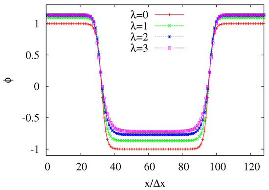
Figure 1. Steady density profiles for different values of the parameter $\lambda$.

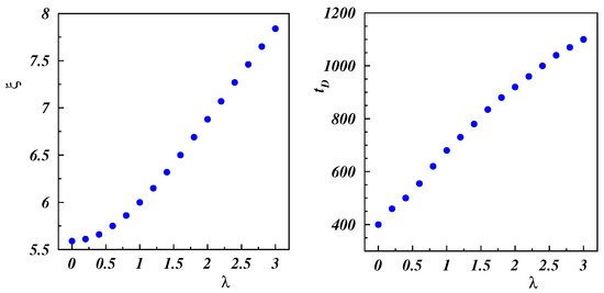
Figure 2. Interface width $\xi$ (left panel) and diffusion time $t_D$ (right panel) as functions of the activity $\lambda$.

The diffusion time $t_D$ is computed as the time for the initial sharp profile to relax to the steady interface (see the Appendix A). Numerical results give $t_D\simeq 4\times {10}^2$ at $\lambda =0$ in agreement with the theoretical estimate of the model B. When $\lambda >0$, it is found that $t_D$ increases with $\lambda$ reaching the highest value $t_D\simeq 1.1\times {10}^3$ when $\lambda =3$. The values of $t_D$ are plotted in the right panel of Figure 2 and show that $t_D$ increases linearly with $\lambda$ up to $\lambda \simeq 1.5$, before slowing down its growth. In the following we consider a range of values of the shear rate between ${\dot{\gamma }}_w=0.9\times {10}^{-3}$ and ${\dot{\gamma }}_s=3.6\times {10}^{-3}$. The values ${\dot{\gamma }}_w$ and ${\dot{\gamma }}_s$ are such to access weak (${\dot{\gamma }}_w{t}_D\left(\lambda \right)\lesssim 1$) and strong (${\dot{\gamma }}_s{t}_D\left(\lambda \right)>1$) shear regimes, respectively, for all considered values of $\lambda$. This guarantees that the shear regime is not affected when changing activity while keeping fixed the strength of applied flow.

3.2. Phase Separation under Weak and Strong Shear

Now we move on to the study of the phase separation under an external shear flow by varying the activity parameter $\lambda$ for $\dot{\gamma }={\dot{\gamma }}_w,{\dot{\gamma }}_s$. We consider a system initially prepared in a symmetric disordered state with $\phi (\mathbf{r},0)=\omega$ where $\omega$ is a random number in the range $[-0.01,0.01]$. This state corresponds to a critical composition of the system. The size of the lattice is $L=1024$ and measures are averaged over five independent runs. The different values of the dimensionless shear rate $\widehat{\dot{\gamma }}$ influence the initial morphology of the forming domains. This can be seen in Figure 3 and Figure 4 where snapshots of systems at consecutive times are shown for the cases at weak ($\dot{\gamma }{t}_D=1.0$) and strong shear ($\dot{\gamma }{t}_D=4.0$), respectively, with $\lambda =3$.

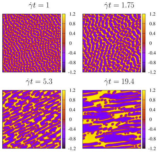
Figure 3. Configurations of the system at consecutive times in the weak shear regime ($\dot{\gamma }{t}_D=1.0$) with $\lambda =3$. A central portion of size $512\times 512$ of the whole lattice is shown.

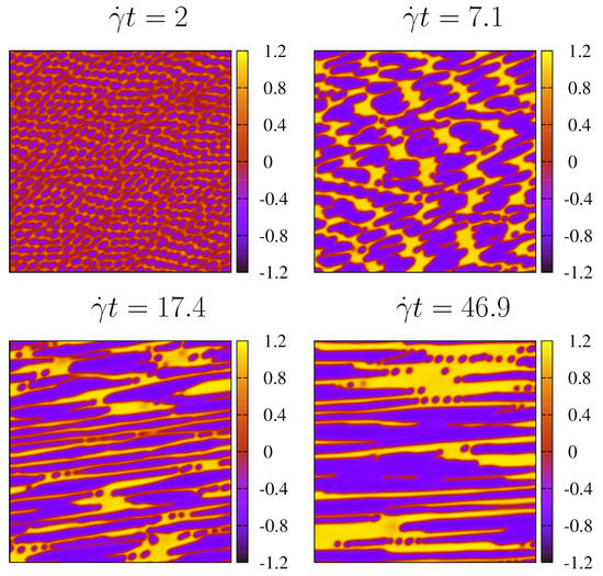
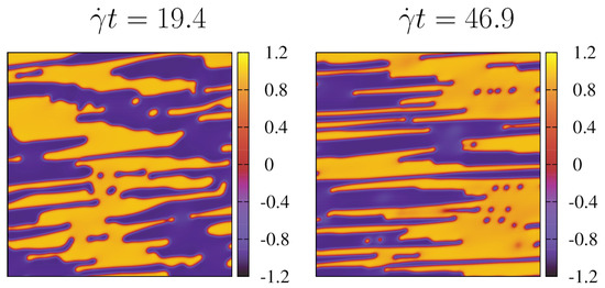
Figure 4. Configurations of the system at consecutive times in the strong shear regime ($\dot{\gamma }{t}_D=4.0$) with $\lambda =3$. A central portion of size $512\times 512$ of the whole lattice is shown.

At weak shear, domains form and grow while the density $\varphi$ attains the steady binodal values before shear effects come into play at values of strain $\dot{\gamma }t>1$. This occurs since the relaxation time scale $t_D\left(\lambda \right)$ is smaller than the shear characteristic time $1/\dot{\gamma }$. Once isolated drops at density ${\varphi }_1$ are produced ($\dot{\gamma }t=1$), the applied flow advects them along the $x-$direction and favours their merging, thus causing the formation of elongated domains along the $y-$direction ($\dot{\gamma }t=1.75$). Afterwards the shear stretches these structures which are tilted as well, being characterized by different thicknesses. Isolated droplets at density ${\varphi }_1$ can be observed inside domains at density ${\varphi }_2$ ($\dot{\gamma }t=5.3$). Later on, the shear further deforms and tilts the domains, which may eventually break up. After the overstretching, domains retract forming ${\varphi }_2$ phases with a larger thickness where isolated droplets of the other phase get trapped ($\dot{\gamma }t=19.4$). Such stretching and bursting persist though this periodic behavior cannot be observed over very long periods of time due to the finite size of the system.

In the strong shear regime, the initial morphology is different with respect to the previous case, since the interface diffusion time is larger than the inverse of the shear rate. Indeed, while domains grow (as quantified later) and start to be deformed by the flow, the two phases are still far from the steady binodal densities (see the panel at $\dot{\gamma }t=2$ in Figure 4), an effect promoting an initial thinning of domains along the shear direction. Afterwards, the elongations and ruptures of domains previously described take place once again, a phenomenon also observed in simulations of passive model B with strong shear [41,42]. However, unlike such cases, the main feature here is that, under shear, isolated droplets of the ${\varphi }_1$ phase survive and are dispersed in the ${\varphi }_2$ matrix (see in particular the last snapshots of Figure 3 and Figure 4). This is not the case if $\lambda =0$, as demonstrated in Figure 5 where instantaneous configurations of the passive case taken at equal times are shown.

Figure 5. Configurations of the system in the weak (left panel, $\dot{\gamma }{t}_D=0.4$) and strong (right panel, $\dot{\gamma }{t}_D=1.4$) shear regimes with $\lambda =0$. Snapshots are taken at the latest times of Figure 3 and Figure 4. A central portion of size $512\times 512$ of the whole lattice is shown.

A scenario akin to that just described in the AMB occurs when considering sheared binary mixtures with surface diffusion [64]. However, in the present work the physical explanation is different. The fraction $\beta$ of the ${\varphi }_1$ phase is larger than the one of the ${\varphi }_2$ phase when $\lambda >0$ despite the fact that we consider a critical system with a symmetric initial composition such that $<\varphi >=0$ (the symbol $<\dots >$ denotes an average over the lattice). Since the dynamics described by Equation (1) is conserved, the average value of the order parameter $\varphi$ is preserved and it has to be $\beta {\varphi }_1+(1-\beta ){\varphi }_2=0$. In a passive mixture the values of the binodals ${\varphi }_1,{\varphi }_2$ are symmetric with respect to the value $\varphi =0$ and it results $\beta =0.5$. In the AMB the binodals are not symmetric anymore with respect to the value $\varphi =0$ and one has $\beta >0.5$, since $|{\varphi }_1|<{\varphi }_2$ when $\lambda >0$. As a result, the ${\varphi }_1$ phase is more abundant than the ${\varphi }_2$ one. In our study it is ${\varphi }_1\simeq -0.71$ and ${\varphi }_2\simeq 1.15$ when $\lambda =3$ so that $\beta \simeq 0.62$. Therefore, in AMB, it is the activity that produces an effective off-symmetric mixture though the initial state is not, in agreement with previous studies of AMB [32]. Such off-symmetric mixture consists of droplets of the majority (${\varphi }_1$) phase dispersed in the minority (${\varphi }_2$) one, a situation persisting under shear. We finally note that a different morphology would be observed in the coarsening of off-symmetric passive mixtures under shear with a similar ratio between the two phases [65]. In this case, at low shear rate small droplets evaporate due to Ostwald ripening, while for strong flows it is the minority phase to be dispersed in a large number of droplets.

3.3. Domain Size

The coarsening dynamics can be investigated by looking at evolution of the typical measures of domains. The sizes $R_x$ and $R_y$ along the flow and the shear directions, respectively, are shown in Figure 6 and are computed as the inverse of the first moments of the structure factor

$$R_{x,y}\left(t\right)=\pi \frac{\int d\mathbf{k}C(\mathbf{k},t)}{\int d\mathbf{k}|k_{x,y}|C(\mathbf{k},t)}.$$

(8)

$C(\mathbf{k},t)=⟨\varphi (\mathbf{k},t)\varphi (-\mathbf{k},t)⟩$ is the structure factor averaged over different realizations of the system and $\varphi (\mathbf{k},t)$ is the Fourier transform of the order parameter.

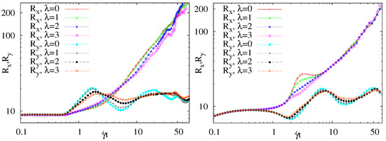
Figure 6. Average measures of domains along the flow ($R_x$) and the shear ($R_y$) directions as functions of time at weak (left panel) and strong (right panel) shear for different values of $\lambda$.

At weak shear, it results that $R_x\simeq R_y$ until $\dot{\gamma }t\lesssim 1$, then $R_y$ grows initially faster than $R_x$ due to the shear-induced dragging of droplets along the flow direction. The typical size along the shear direction attains a maximum at $\dot{\gamma }t\simeq 1.75$ and then decreases, while the growth rate along the flow direction increases due to shear stretching. The quantity $R_y$ oscillates on a logarithmic time scale between minimum and maximum values corresponding to elongated and broken domains, respectively. The amplitude of such oscillations diminishes when increasing the activity parameter $\lambda$ and is related to the existence of small droplets that cannot grow any further. The radii $R_x$ for different values of $\lambda$ show a similar trend compatible with an asymptotic power-law growth $R_x\sim A\left(\lambda \right)t^{{\alpha }_x}$. Fitting the power law for $R_x$ to numerical data shows that the amplitudes A decrease with the activity as illustrated in Table 1, while the exponent ${\alpha }_x\simeq 1$ does not seem to be affected by $\lambda$.

Table 1. Fitted values of the amplitudes A for different values of the activity $\lambda$ in the weak shear regime.

$\mathit{\lambda }$	A
0	4.40
1	2.75
2	0.99
3	0.82

Due to the limited size of the simulated system and the superimposed oscillations, it is difficult to estimate the growth exponent ${\alpha }_y$ along the shear direction although, at $\dot{\gamma }t\gtrsim 5$, one observes a regime with ${\alpha }_x-{\alpha }_y\simeq 1$. This result is due to the advection of domains by the applied flow, and has been observed in the passive model B under shear as well [41,42].

At increasing values of shear rate, the growth along the flow direction proceeds faster than that in the shear direction, with a local maximum of $R_x$ at $\dot{\gamma }t\simeq 3$ corresponding to a minimum for $R_y$, since domains are strongly deformed by the shear. Note that the height of the maximum of $R_x$ is reduced by increasing the activity, a feature associated to the presence of droplets which can be deformed only slightly by the flow. When $\dot{\gamma }t\gtrsim 7$, $R_x$ shows a power-law growth with an exponent ${\alpha }_x\simeq 1.1$ not depending on $\lambda$, while the size $R_y$ exhibits a periodic behavior on a logarithmic time scale with amplitude that shrinks with $\lambda$. By using power counting, it might be expected that the net effect of the convective term is to increase the growth exponent of the unsheared system by 1 in the flow direction. However, as previously discussed, in AMB with no external flow the value of the growth exponent has not been definitely determined yet. Our results seem to point towards a picture in which the activity has mild effect on the coarsening dynamics, as in the unsheared case [32], since we find that ${\alpha }_x\simeq 1$ as in the passive case and ${\alpha }_x-{\alpha }_y\simeq 1$. Additional simulations run on systems of size $L=512$ do not provide further insights for evaluating ${\alpha }_x$ and ${\alpha }_y$ as well as for attempting a finite-size scaling analysis. Indeed, a more accurate estimate of the growth exponents would likely require much larger systems, thus dramatically increasing the computational resources necessary to simulate their late-time dynamics.

To elucidate the role of flow strength, simulations with shear rate $\dot{\gamma }=2.8\times {10}^{-3}$ are also considered. This value is such that $\dot{\gamma }{t}_D\left(\lambda \right)\gtrsim 1.1$ for $0\le \lambda \le 3$ so that the system is in the strong regime. The time behavior of $R_x$ and $R_y$ is similar to the one shown in Figure 6, with no significant effect on the growth exponents. We only observe a reduction in the amplitudes of oscillations at the smallest values of activity along the x-direction, since domains are less affected by flow. Being less deformed, they can grow along the shear direction, a result witnessed by wider amplitudes of $R_y$ with respect to the case with $\dot{\gamma }=3.6\times {10}^{-3}$. These effects reduce when $\lambda$ increases, since, as previously discussed, the dynamics is deeply modified by the presence of droplets for the highest value of activity.

The size distribution of domains can be analyzed by calculating the normalized probability distributions $P\left(L_{x,y}\right)$, having domains of lengths $L_x$ and $L_y$ along the flow and the shear directions, respectively. By moving along all rows (the flow direction) of the computational domain, $L_x$ is computed as the size of unidimensional domains with equal composition (same sign of the density $\varphi$). From the registered values of $L_x$, the function $P\left(L_x\right)$ is derived. The same procedure is adopted along the columns (the shear direction) of the lattice to determine $L_y$ and then $P\left(L_y\right)$. In Figure 7 and Figure 8 we plot $P\left(L_x\right)$ and $P\left(L_y\right)$ for $\lambda =0.3$ in the weak and strong shear regime. At weak shear (see Figure 7), $P\left(L_x\right)$ and $P\left(L_y\right)$ show two peaks in the active case and a single one in the passive situation. The peaks at the smaller values of $L_x$ and $L_y$ (with $L_x\simeq L_y\simeq 8$) correspond to the presence of isolated droplets, while the other peaks indicate elongated domains. In particular, $P\left(L_x\right)$ broadens when going from the maximum of $R_y$ at $\dot{\gamma }t\simeq 1.75$ to the minimum at $\dot{\gamma }t\simeq 5.3$ and, then, shrinks when $R_y$ grows again. In the passive counterpart, the distribution functions are less broad. When looking at the shear direction, in the active case the peak of $P\left(L_y\right)$ at the larger value of $L_y$ oscillates in height, with a local maximum attained when $R_y$ is at the minimum ($\dot{\gamma }t\simeq 5.3$). Later $P\left(L_y\right)$ broadens. In the passive case the distribution $P\left(L_y\right)$ has a single peak (narrower than in the active case) that oscillates in height, following the cyclic dynamics of elongations and ruptures.

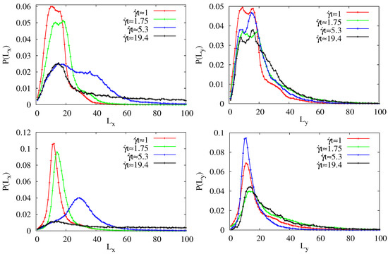
Figure 7. Probability distribution functions P of domains of length $L_x$ (left panels) and $L_y$ (right panels) with $\lambda =3$ (upper row) and $\lambda =0$ (lower row) in the weak shear regime.

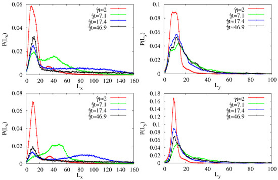
Figure 8. Probability distribution functions P of domains of length $L_x$ (left panels) and $L_y$ (right panels) with $\lambda =3$ (upper row) and $\lambda =0$ (lower row) in the strong shear regime.

Moving to the strong shear regime (Figure 8), we observe that $P\left(L_x\right)$ is characterized by the presence of two peaks both in the passive and in the active case, roughly at the same positions. When $\lambda =3$, the peak at $L_x\simeq 10$ is always the prevailing one, owing to the presence of droplets spanning the system. The value of $L_x$, corresponding to the second peak, increases in time attaining its maximum at $\dot{\gamma }t\simeq 17.4$, when domains are highly stretched ($R_y$ is at its minimum). The subsequent breaking-up of domains determines the shift in position of the second peak to smaller values. Moreover, it can be seen that the distributions are broader in the active case. This feature also holds for $P\left(L_y\right)$, whose main peak oscillates in height during the time evolution. We note here that in the active system the first peak of $P\left(L_y\right)$ at the smaller value of $L_y$, corresponding to isolated droplets, is less pronounced with respect to that of the weak shear regime. This can be attributed to the fact that, as previously discussed, initially forming droplets are fused by shear before growing in size.

4. Conclusions

To summarize, we have investigated the phase separation of an active binary mixture subject to an applied shear flow. For this purpose we numerically solved the phenomenological equation of the active model B [32], supplemented by a convective term that couples the order parameter to the external velocity field. The initial morphology depends on the strength of shear. Later, growing domains are elongated, tilted, and burst by the flow. This is reflected in the typical sizes of domains $R_x$ and $R_y$ along the two spatial dimensions, which appear to be modulated by oscillations on a logarithmic time scale. However, the presence of activity is such that the fraction of one phase is larger than the other one, despite the initial symmetric composition. This induces the presence of droplets of the more abundant phase which span the system and are responsible for the observed reduction of the amplitudes of the oscillations of $R_x$ and $R_y$ when increasing the activity parameter. Though the limited size of the simulated system does not allow an estimate of the growth exponents ${\alpha }_x$ and ${\alpha }_y$ along the flow and the shear directions, respectively, we find that ${\alpha }_x-{\alpha }_y\simeq 1$ as in the passive case [41,42]. The combined effect of activity and shear on the overall morphology has been studied by considering the probability distribution functions (PDFs) of the size of patterns along the two spatial directions. Our simulations suggest that such PDFs are characterized by a width that broadens with activity.

We hope that our results may stimulate further research on this system. It would be of interest, for example, understanding the role played by the shear in active binary mixtures where all terms breaking time-reversal symmetry to leading order in ∇ and $\varphi$ are included [28], as well as how thermal noise is expected to impact on morphology and growth dynamics in the presence of an external driving.

References

- Ramaswamy, S. The Mechanics and Statistics of Active Matter. Annu. Rev. Condens. Mat. Phys. 2010, 1, 323–345. [Google Scholar] [CrossRef]
- Romanczuk, P.; Bär, M.; Ebeling, W.; Lindner, B.; Schimansky-Geier, L. Active Brownian particles. Eur. Phys. J. Spec. Top. 2012, 202, 1–62. [Google Scholar] [CrossRef]
- Marchetti, M.C.; Joanny, J.F.; Ramaswamy, S.; Liverpool, T.B.; Prost, J.; Rao, M.; Sima, R.A. Hydrodynamics of soft active matter. Rev. Mod. Phys. 2013, 85, 1143. [Google Scholar] [CrossRef]
- Bechinger, C.; Leonardo, R.D.; Löwen, H.; Reichhardt, C.; Volpe, G.; Volpe, G. Active particles in complex and crowded environments. Rev. Mod. Phys. 2016, 88, 045006. [Google Scholar] [CrossRef]
- Ramaswamy, S. Active fluids. Nat. Rev. Phys. 2019, 1, 640. [Google Scholar] [CrossRef]
- Leonardo, R.D.; Angelani, L.; Dell’Arciprete, D.; Ruocco, G.; Iebba, V.; Schippa, S.; Conte, M.P.; Mecarini, F.; Angelis, F.D.; Fabrizio, E.D. Bacterial ratchet motors. Proc. Nat. Acad. Sci. USA 2010, 107, 9541. [Google Scholar] [CrossRef]
- Sanchez, T.; Chen, D.T.N.; DeCamp, S.J.; Heymann, M.; Dogic, Z. Spontaneous motion in hierarchically assembled active matter. Nature 2012, 491, 431. [Google Scholar] [CrossRef]
- López, H.M.; Gachelin, J.; Douarche, C.; Auradou, H.; Clément, E. Turning Bacteria Suspensions into Superfluids. Phys. Rev. Lett. 2015, 115, 028301. [Google Scholar] [CrossRef]
- Dell’Arciprete, D.; Blow, M.L.; Brown, A.T.; Farrell, F.D.C.; Lintuvuori, J.S.; McVey, A.S.; Marenduzzo, D.; Poon, W.C.K. A growing bacterial colony in two dimensions as an active nematic. Nat. Commun. 2018, 9, 1. [Google Scholar] [CrossRef]
- Theurkauff, I.; Cottin-Bizonne, C.; Palacci, J.; Ybert, C.; Bocquet, L. Dynamic Clustering in Active Colloidal Suspensions with Chemical Signaling. Phys. Rev. Lett. 2012, 108, 268303. [Google Scholar] [CrossRef]
- Buttinoni, I.; Bialké, J.; Kümmel, F.; Löwen, H.; Bechinger, C.; Speck, T. Dynamical Clustering and Phase Separation in Suspensions of Self-Propelled Colloidal Particles. Phys. Rev. Lett. 2013, 110, 238301. [Google Scholar] [CrossRef]
- Palacci, J.; Sacanna, S.; Steinberg, A.P.; Pine, D.J.; Chaikin, P.M. Living crystals of light-activated colloidal surfers. Science 2013, 339, 936. [Google Scholar] [CrossRef] [PubMed]
- Needleman, D.; Dogic, Z. Active particles induce large shape deformations in giant lipid vesicles. Nat. Rev. Mater. 2017, 2, 17048. [Google Scholar] [CrossRef]
- Saw, T.B.; Doostmohammadi, A.; Nier, V.; Kocgozlu, L.; Thampi, S.; Toyama, Y.; Marcq, P.; Lim, C.T.; Yeomans, J.M.; Ladoux, B. Topological defects in epithelia govern cell death and extrusion. Nature 2017, 544, 212. [Google Scholar] [CrossRef] [PubMed]
- Shaebani, M.R.; Wysocki, A.; Winkler, R.G.; Gompper, G.; Rieger, H. Computational models for active matter. Nat. Rev. Phys. 2020, 2, 181. [Google Scholar] [CrossRef]
- Tailleur, J.; Cates, M.E. Statistical Mechanics of Interacting Run-and-Tumble Bacteria. Phys. Rev. Lett. 2008, 100, 218103. [Google Scholar] [CrossRef] [PubMed]
- Cates, M.E.; Tailleur, J. Motility-Induced Phase Separation. Annu. Rev. Cond. Matt. Phys. 2015, 6, 219–244. [Google Scholar] [CrossRef]
- Gonnella, G.; Marenduzzo, D.; Suma, A.; Tiribocchi, A. Motility-induced phase separation and coarsening in active matter. Compt. Ren. Phys. 2015, 16, 316. [Google Scholar] [CrossRef]
- Fily, Y.; Marchetti, M.C. Athermal Phase Separation of Self-Propelled Particles with No Alignment. Phys. Rev. Lett. 2012, 108, 235702. [Google Scholar] [CrossRef]
- Stenhammar, J.; Tiribocchi, A.; Allen, R.J.; Marenduzzo, D.; Cates, M.E. Continuum Theory of Phase Separation Kinetics for Active Brownian Particles. Phys. Rev. Lett. 2013, 111, 145702. [Google Scholar] [CrossRef]
- Stenhammar, J.; Allen, R.J.; Marenduzzo, D.; Cates, M.E. Phase behaviour of active Brownian particles: The role of dimensionality. Soft Matter 2014, 10, 1489. [Google Scholar] [CrossRef]
- Speck, T.; Bialké, J.; Menzel, A.M.; Löwen, H. Effective Cahn-Hilliard Equation for the Phase Separation of Active Brownian Particles. Phys. Rev. Lett. 2014, 112, 218304. [Google Scholar] [CrossRef]
- Fodor, E.; Nardini, C.; Cates, M.E.; Tailleur, J.; Visco, P.; van Wijland, F. How Far from Equilibrium Is Active Matter? Phys. Rev. Lett. 2016, 117, 038103. [Google Scholar] [CrossRef] [PubMed]
- Nardini, C.; Fodor, E.; Tjhung, E.; van Wijland, F.; Tailleur, J.; Cates, M.E. Entropy Production in Field Theories without Time-Reversal Symmetry: Quantifying the Non-Equilibrium Character of Active Matter. Phys. Rev. X 2017, 7, 021007. [Google Scholar] [CrossRef]
- Takatori, S.C.; Yan, W.; Brady, J.F. Swim Pressure: Stress Generation in Active Matter. Phys. Rev. Lett. 2014, 113, 028103. [Google Scholar] [CrossRef]
- Solon, A.P.; Chaté, H.; Tailleur, J. From Phase to Microphase Separation in Flocking Models. Phys. Rev. Lett. 2015, 114, 068101. [Google Scholar] [CrossRef] [PubMed]
- Ginot, F.; Theuekauff, I.; Levis, D.; Ybert, C.; Bocquet, L.; Berthier, L.; Cottin-Bizonne, C. Nonequilibrium Equation of State in Suspensions of Active Colloids. Phys. Rev. X 2015, 5, 011004. [Google Scholar] [CrossRef]
- Tjhung, E.; Nardini, C.; Cates, M.E. Cluster Phases and Bubbly Phase Separation in Active Fluids: Reversal of the Ostwald Process. Phys. Rev. X 2018, 8, 031080. [Google Scholar] [CrossRef]
- Caporusso, C.B.; Digregorio, P.; Levis, D.; Cugliandolo, L.F.; Gonnella, G. Motility-Induced Microphase and Macrophase Separation in a Two-Dimensional Active Brownian Particle System. Phys. Rev. Lett. 2020, 125, 178004. [Google Scholar] [CrossRef]
- Shi, X.-Q.; Fausti, G.; Chaté, H.; Nardini, C.; Solon, A. Self-Organized Critical Coexistence Phase in Repulsive Active Particles. Phys. Rev. Lett. 2020, 125, 168001. [Google Scholar] [CrossRef]
- Cates, M.E. Active Field Theories. arXiv 2019, arXiv:1904.01330. [Google Scholar]
- Wittkowski, R.; Tiribocchi, A.; Stenhammar, J.; Allen, R.J.; Marenduzzo, D.; Cates, M.E. Scalar φ4 field theory for active-particle phase separation. Nat. Comm. 2014, 5, 4351. [Google Scholar] [CrossRef] [PubMed]
- Hohenberg, P.C.; Halperin, B.I. Theory of dynamic critical phenomena. Rev. Mod. Phys. 1977, 49, 435. [Google Scholar] [CrossRef]
- Cahn, J.W.; Hilliard, J.E. Free Energy of a Nonuniform System. I. Interfacial Free Energy. J. Chem. Phys. 1958, 28, 258. [Google Scholar] [CrossRef]
- Cahn, J.W.; Hilliard, J.E. Free Energy of a Nonuniform System. III. Nucleation in a Two-Component Incompressible Fluid. J. Chem. Phys. 1959, 31, 688. [Google Scholar] [CrossRef]
- Bray, J. Theory of phase-ordering kinetics. Adv. Phys. 1994, 43, 357. [Google Scholar] [CrossRef]
- Otha, T.; Nozaki, H.; Doi, M. Computer simulations of domain growth under steady shear flow. J. Chem. Phys. 1990, 93, 2664. [Google Scholar]
- Corberi, F.; Gonnella, G.; Lamura, A. Spinodal Decomposition of Binary Mixtures in Uniform Shear Flow. Phys. Rev. Lett. 1998, 81, 3852. [Google Scholar] [CrossRef]
- Corberi, F.; Gonnella, G.; Lamura, A. Structure and Rheology of Binary Mixtures in Shear Flow. Phys. Rev. E 2000, 61, 6621. [Google Scholar] [CrossRef]
- Berthier, L. Phase separation in a homogeneous shear flow: Morphology, growth laws, and dynamic scaling. Phys. Rev. E 2001, 63, 051503. [Google Scholar] [CrossRef]
- Corberi, F.; Gonnella, G.; Lamura, A. Two-Scale Competition in Phase Separation with Shear. Phys. Rev. Lett. 1999, 83, 4057. [Google Scholar] [CrossRef]
- Corberi, F.; Gonnella, G.; Lamura, A. Phase Separation of Binary Mixtures in Shear Flow: A Numerical Study. Phys. Rev. E 2000, 62, 8064. [Google Scholar] [CrossRef] [PubMed]
- Gonnella, G.; Lamura, A. Long-time behavior and different shear regimes in quenched binary mixtures. Phys. Rev. E 2007, 75, 011501. [Google Scholar] [CrossRef] [PubMed]
- Rothman, D.H. Complex rheology in a model of a phase-separating fluid. Europhys. Lett. 1991, 14, 337. [Google Scholar] [CrossRef]
- Hashimoto, T.; Matsuzaka, K.; Moses, E.; Onuki, A. String Phase in Phase-Separating Fluids under Shear Flow. Phys. Rev. Lett. 1995, 74, 126. [Google Scholar] [CrossRef]
- Nakano, H.; Minami, Y.; Sasa, S. Long-Range Phase Order in Two Dimensions under Shear Flow. Phys. Rev. Lett. 2021, 126, 160604. [Google Scholar] [CrossRef]
- Saracco, G.P.; Gonnella, G. Critical behavior of the Ising model under strong shear: The conserved case. Phys. A 2021, 576, 126038. [Google Scholar] [CrossRef]
- Stenhammar, J.; Wittkowski, R.; Marenduzzo, D.; Cates, M.E. Activity-Induced Phase Separation and Self-Assembly in Mixtures of Active and Passive Particles. Phys. Rev. Lett. 2015, 114, 018301. [Google Scholar] [CrossRef]
- Cates, M.E.; Tjhung, E. Theories of binary fluid mixtures: From phase-separation kinetics to active emulsions. J. Fluid Mech. 2018, 836, P1. [Google Scholar] [CrossRef]
- Caballero, F.; Nardini, C.; Cates, M.E. From bulk to microphase separation in scalar active matter: A perturbative renormalization group analysis. J. Stat. Mech. 2018, 2018, 123208. [Google Scholar] [CrossRef]
- Solon, A.P.; Stenhammar, J.; Cates, M.E.; Kafri, Y.; Tailleur, J. Generalized thermodynamics of phase equilibria in scalar active matter. Phys. Rev. E 2018, 97, 020602R. [Google Scholar] [CrossRef]
- Pattanayak, S.; Mishra, S.; Puri, S. Ordering kinetics in the active model B. Phys. Rev. E 2021, 104, 014606. [Google Scholar] [CrossRef] [PubMed]
- Pattanayak, S.; Mishra, S.; Puri, S. Domain Growth in the Active Model B: Critical and Off-critical Composition. Soft Mater. 2021, 19, 286. [Google Scholar] [CrossRef]
- Redner, G.S.; Hagan, M.F.; Baskaran, A. Structure and Dynamics of a Phase-Separating Active Colloidal Fluid. Phys. Rev. Lett. 2013, 110, 055701. [Google Scholar] [CrossRef]
- Tiribocchi, A.; Wittkowski, R.; Marenduzzo, D.; Cates, M.E. Scalar Active Matter in a Momentum-Conserving Fluid. Phys. Rev. Lett. 2015, 115, 188302. [Google Scholar] [CrossRef]
- Kardar, M.; Parisi, G.; Zhang, Y.-C. Dynamic Scaling of Growing Interfaces. Phys. Rev. Lett. 1986, 56, 889. [Google Scholar] [CrossRef] [PubMed]
- Hunter, J.K.; Saxton, R. Dynamics of Director Fields. Siam J. Appl. Math. 1991, 51, 1498. [Google Scholar] [CrossRef]
- Kuramoto, Y. Diffusion-Induced Chaos in Reaction Systems. Prog. Theor. Phys. Suppl. 1978, 64, 346. [Google Scholar] [CrossRef]
- Sivashinsky, G.I. On Flame Propagation Under Conditions of Stoichiometry. Siam J. Appl. Math. 1980, 39, 67. [Google Scholar] [CrossRef]
- Rogers, T.M.; Elder, K.R.; Desai, R.C. Numerical study of the late stages of spinodal decomposition. Phys. Rev. B 1988, 37, 9638. [Google Scholar] [CrossRef]
- Strikwerda, J.C. Finite Difference Schemes and Partial Differential Equations; Chapman and Hall: New York, NY, USA, 1989. [Google Scholar]
- Lees, A.W.; Edwards, S.F. The computer study of transport processes under extreme conditions. J. Phys. C 1972, 5, 1921. [Google Scholar] [CrossRef]
- Frischknecht, A. Effect of shear flow on the stability of domains in two-dimensional phase-separating binary fluids. Phys. Rev. E 1997, 56, 6970. [Google Scholar] [CrossRef]
- Gonnella, G.; Lamura, A. Sheared phase-separating binary mixtures with surface diffusion. J. Phys. A 2020, 53, 305002. [Google Scholar] [CrossRef]
- Lamura, A.; Gonnella, G. Computer simulations of domain growth in off-critical quenches of two-dimensional binary mixtures. Comput. Mater. 2002, 25, 531. [Google Scholar] [CrossRef][Green Version]
Publisher’s Note: MDPI stays neutral with regard to jurisdictional claims in published maps and institutional affiliations. |
© 2021 by the authors. Licensee MDPI, Basel, Switzerland. This article is an open access article distributed under the terms and conditions of the Creative Commons Attribution (CC BY) license (https://creativecommons.org/licenses/by/4.0/).