Abstract
This article shows a new Te-transform and its periodogram for applications that mainly exhibit stochastic behavior with a signal-to-noise ratio lower than −30 dB. The Te-transform is a dyadic transform that combines the properties of the dyadic Wavelet transform and the Fourier transform. This paper also provides another contribution, a corollary on the energy relationship between the untransformed signal and the transformed one using the Te-transform. This transform is compared with other methods used for the analysis in the frequency domain, reported in literature. To perform the validation, the authors created two synthetic scenarios: a noise-free signal scenario and another signal scenario with a signal-to-noise ratio equal to −69 dB. The results show that the Te-transform improves the sensitivity in the frequency spectrum with respect to previously reported methods.
1. Introduction
This paper presents three contributions. The first one is directed at a new dyadic Te-transform (DTeT). The second addresses the dyadic Te-periodogram (DTeP), and the last contribution shows a corollary on the energy conservation of the transformed signal by Te-transform. To carry out this work, the authors relied on the properties of the Fourier transform (FT), the dyadic Wavelet transform (DWT), and the Welch–Bartlett periodogram (WBP).
The dyadic Wavelet transform allows a signal to be analyzed by decomposing it into scales or decomposition levels [1,2,3], which provides a representation with variable sensitivity. On the other hand, the Fourier transform and the Welch–Bartlett periodogram provide information about the frequency components present in a signal.
At present, the analysis of a signal in the frequency domain is commonly used to extract characteristics in deterministic and stochastic processes. The authors in [4,5] present an article with a bibliographic review aimed at detecting a spectrum in cognitive radio. These researchers state that the main challenge in their field of research is to address the detection of signals with a signal-to-noise ratio (SNR) lower than zero. The bibliographic review shown in [6] is directed at vibration monitoring and signal processing methods. Its authors state that vibrations are directly related to mechanical disturbances by various sources such as motor, sound, noise, etc., which cause a decrease in the signal-to-noise ratio.
As we can see, it is very important to have mathematical tools that allow detecting the presence of a signal under the condition of a signal-to-noise ratio below zero, despite the fact that, at present, this problem still exists; many researchers continue to extract characteristics using traditional methods.
The research in [7] shows a work focused on the short-time adaptive Fourier transform and the synchronized compression transform for the separation of non-stationary signals. These researchers in their proposal only work with SNR ≥ 0 dB. For their part, the authors in [8] created an algorithm using the short-time Fourier transform for the diagnosis of transient states in a hydraulic pump system. In the results presented by these researchers, it is observed that when noise begins to increase, there is deterioration in the extraction of characteristics of the studied signal. Shuang Zhou et al. in [9] proposed an algorithm for the prediction of the useful life and the diagnosis of bearing failures. This procedure is based on the short-time Fourier transform.
On the other hand, many authors prefer to use the Welch–Bartlett periodogram to analyze signals with a signal-to-noise ratio below zero. This is due to the fact that the principle of operation of said periodogram is based on overlapping the windows by 50%. The authors of [10] conducted a study on passive impedance spectroscopy to monitor lithium-ion battery cells during vehicle operation. These researchers claim that the use of the Welch–Bartlett periodogram provides noise attenuation due to 50% overlap. Blaise Kévin Guépié et al. [11] presented an article focused on leak detection in a heat exchanger of a sodium-cooled fast reactor. The main contribution of these authors is that their proposal allows the extraction of features with SNR ≥ −30 dB.
In [12] results are presented on the separation characteristics between the time domain and the frequency domain for a signal from a wind farm. These authors in their study used the discrete Wavelet transform to analyze the time domain and the Welch–Bartlett periodogram to analyze the frequency domain.
However, in other applications, many researchers focus their proposal on the use of the spectrogram or the scalogram. The manuscript shown in [13] gives a proposal to predict bearing failures. Said researchers claim that the spectrogram is a good method to analyze the vibration signal with background noise. The authors in [14] show a procedure in which their main objective is to represent a spectrogram based on a method evaluated as an image to support transient analysis on rotating machines. In this work, they detect the presence of a signal with an SNR ≥ −22.9 dB. Thanh Tran and Jan Lundgren in [15] show a drilling fault diagnosis method based on scalogram and spectrogram of sound signals. These authors state that in industry, the ability to detect damage or abnormal operation in machinery is very important; however, they do not show the performance of their method with a signal-to-noise ratio below zero.
Researchers in [16] show a work on the application of the adaptive Wavelet transform for the diagnosis of gear failures using a filtered vibration signal. These authors state that the scalogram is excellent for analyzing signals with a signal-to-noise ratio below zero.
The main drawback of these methods is that they do not allow analyzing signals in the frequency domain maximizing the detection sensitivity, which allows to analyze signals with an SNR ≥ −69 dB attenuating cross-terms and also to isolate the frequency component, as shown in the section on validation.
The rest of the manuscript is organized as follows. Section 2 contains the definitions for the Te-transform. Section 3 shows the properties for the dyadic Te-transform. Section 4 shows the dyadic Te-periodogram (DTeP). Section 5 shows the validation for dyadic Te-transform and the dyadic Te-periodogram (DTeP). Finally, the main conclusions are shown in Section 6.
2. Definitions
This section shows the definitions used for a signal contained in a Hilbert space (). These definitions are used to prove the dyadic Te-transform in Section 3.
Fourier and Wavelet Transforms
Definition 1.
(Linear operator [17,18]): if , a linear operator from is mapping such that:
Definition 2.
(Hermitian symmetry [19]): the Fourier transform of a has Hermitian symmetry, such that:
where: is Fourier transform, represents frequency in Hz, and is the complex conjugate of .
Definition 3.
(Invariant operator [18,20]): if the for a signal shifted is:
Convolution theorem [3]: let z and function is in then:
where: is Fourier transform for h, and is Fourier transform for .
Definition 4.
(Time-frequency resolution [3]): a time-frequency dictionary is composed of waveforms of unit norm , which have a narrow localization in time and frequency. The time localization and spread around u are defined by:
Similarly, the frequency localization and spread of are defined by:
Definition 5.
(Parseval’s Theorem [3,18]): if , then:
where: is the Fourier transform of .
Definition 6.
(Generalities about frames [3,21]): a family of functions is called a frame if there exist and so that :
where: A and B are the frame bounds.
3. Dyadic Te-Transform
In this section, the authors present the Te-transform and its properties. Equations (11) and (12) show the short-time Fourier transform (STFT) and the dyadic Wavelet transform (DWT), respectively, for an [1,2,3,18,22,23,24].
where: is a window function, and is the short-time Fourier transform for .
where: is a dyadic wavelet, and are the scale and translation parameters, respectively, and is dyadic Wavelet transform of .
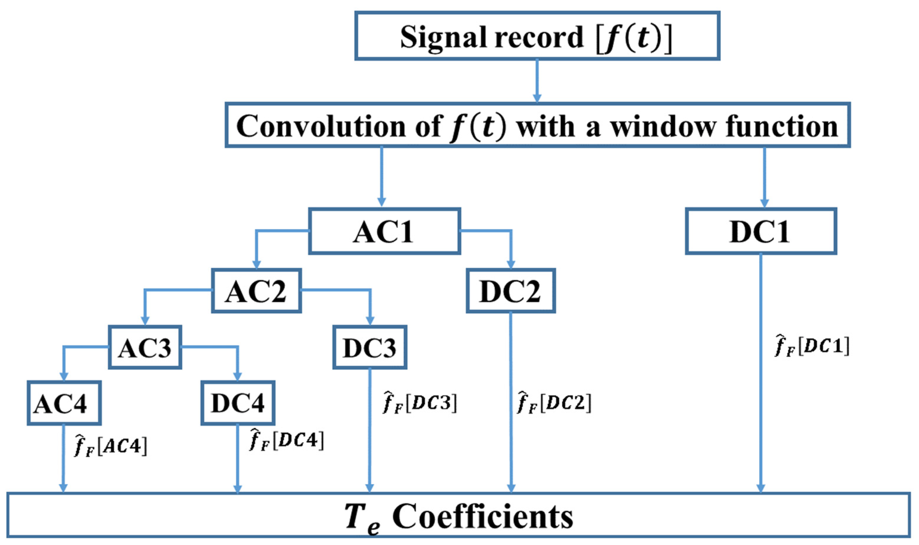
Since the short-time Fourier transform and the dyadic Wavelet transform are integrated into the same domain, can be integrated by both transforms, leading to the new dyadic Te-transform (see Equation (13)). The dyadic Te-transform analyzes the behavior of a signal in the Te-dyadic domain, having the main advantage of maximizing the sensitivity of the analysis. Figure 1 shows a graphical description of the dyadic Te-transform.
where: is the dyadic Te-transform of , and denotes the dyadic linear frequency.
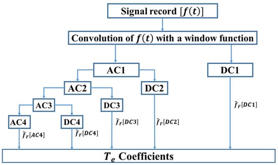
Figure 1.
Decomposition tree of the dyadic Te-transform, AC are the approximation coefficients, and DC are the detail coefficients.
3.1. Inverse Dyadic Te-Transform
To obtain the inverse of the dyadic Te-transform (iDTe), the authors used Figure 1, starting from the Te coefficients to the signal to be recovered, and the papers reported in [3,21,22]. First, they analyzed how to recover the signal using the dyadic Wavelet transform, see Equation (14). Then, they analyzed how to recover a signal in convolution with a function from the Fourier transform, see Equation (15). Equation (17) shows the inverse of the dyadic Te-transform.
In order to:
where: is the dual function of and are the dyadic wavelet coefficients.
Equation (15) shows how a convoluted signal is recovered from its frequency spectrum.
where: is short-time Fourier transform of , is the result of the convolution of with . After deconvolutioning , through Equation (16) we get .
where: is the deconvolution operation of . After carrying out these processes, we obtain an expression enabling us to recover the signal with a minimal error by means of the inverse of the dyadic Te-transform, shown in Equation (17).
where: are the Te coefficients.
3.2. Properties of the Dyadic Te-Transform
In this subsection, the properties corresponding to the dyadic Te-transform are shown. For this the authors relied on the properties shown in Section 2.
Definition 1 (Linearity property):
For , and :
Definition 2 (Hermitian symmetry):
To demonstrate this property we start from Equation (18):
Real part Symmetric (even):
Imaginary part Antisymmetric (odd):
Magnitude Symmetric (even):
Phase Antisymmetric (odd):
Definition 3 (Invariant operator):
To demonstrate this property, we translate the signal by , then :
Definition 4 (Time-frequency resolution):
The authors of [1,2,3] state that the time-frequency resolution depends on the time-frequency spread of the dictionary. Our dictionary is:
This implies that:
In this case we use the convolution theorem and the property shown by Mallat in [3] on the Fourier transform of a Wavelet, :
The result obtained on the time-frequency resolution shows that the dyadic Te-transform allows you to analyze signals with multi-sensitivity.
In order to obtain the time-frequency representation of DTe, the authors followed [3] to propose that the probability density of our dictionary being found in t is , where . The probability density that its momentum is equal to is . If we take into account the variance around the average values obtained for our dictionary, we obtain Equations (19) and (20):
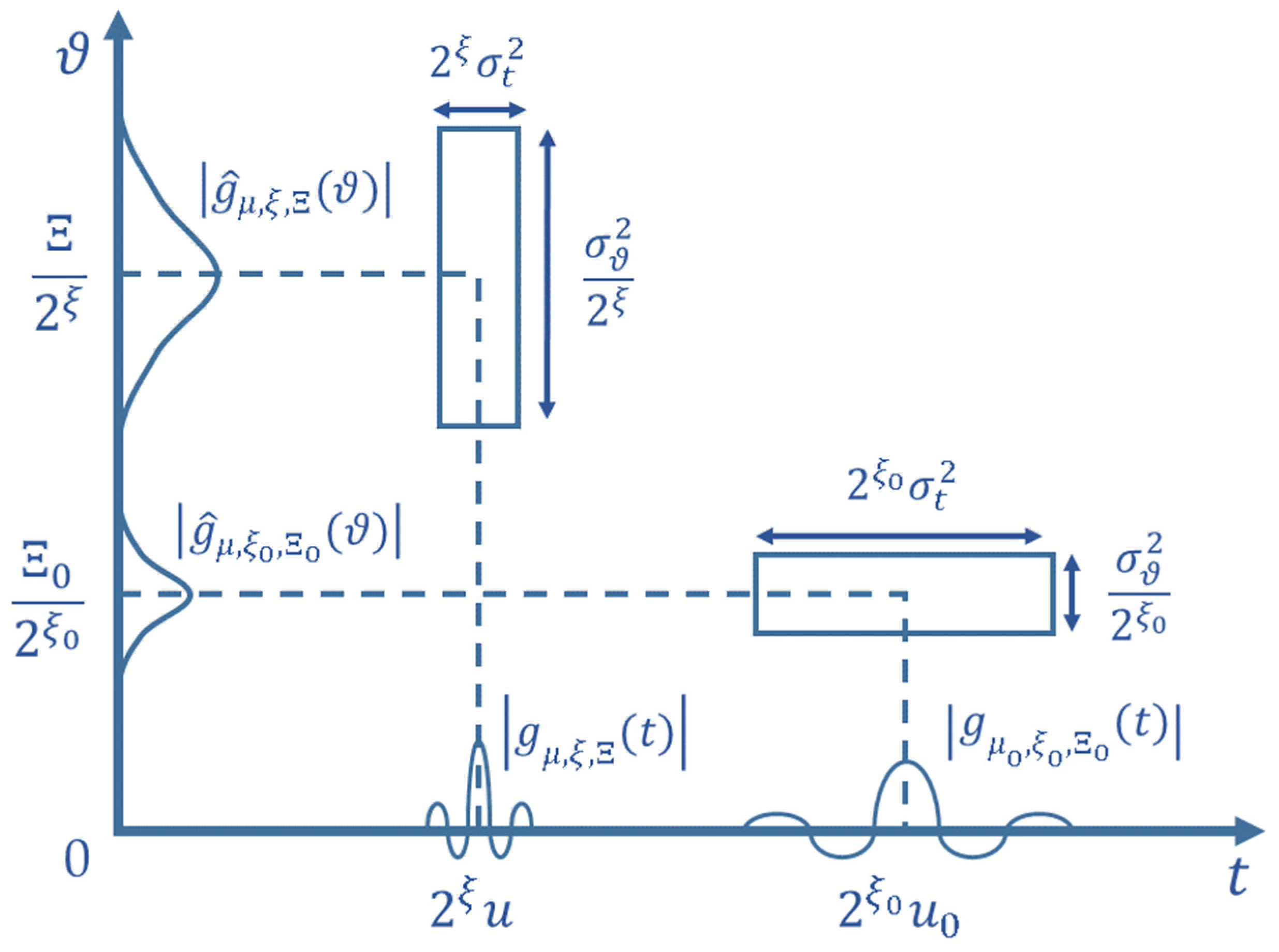
where: and are the location and moment averages, respectively. For the case of analysis we will take the instant where . Applying the Heisenberg Uncertainty theorem and the results obtained by [3] we obtain the condition shown in Equation (21). This result shows that our dictionary forms a Heisenberg box centered at () as shown in Figure 2.

Figure 2.
Time-frequency representation of .
3.3. Energy Analysis
In this subsection, the Parseval relation and the frame definition are used to propose a corollary. The authors of [3,21] state that when the limits of a frame shown in Definition 6, Section 2 are equal, the frame is called narrow, as shown in Equation (22).
On the other hand, if then the frame is an orthonormal basis and is represented by dyadic wavelets [25,26,27]. If we rewrite Equation (22) for orthonormal bases, we can reach the conclusion that the use of dyadic wavelet does not modify the energy of the transformed signal (see Equation (23)).
where: is a multi-index parameter, denotes the energy of the transformed signal , and denotes the energy of the untransformed signal [3].
If we calculate the energy of the transformed signal by means of the dyadic Te-transform using Equation (24) and the concept explained in Section 2 on Parseval’s theorem, we obtain:
Then, we substitute Equation (13) in Equation (24), obtaining Equation (25):
Considering the Euler identity, Equation (25) is reduced to Equation (26):
Assuming that is a unit-norm window function, which implies that its energy is the unit and that is an orthonormal function, from Equation (26) the relationship shown in Equation (27) is deduced.
This result shows that the dyadic Te-transform does not modify the energy of the signal in its transformation, which allows the authors to propose the following corollary.
Corollary: Given that the dyadic Te-transform uses orthonormal bases and , the energy of the transformed signal is unchanged, Equation (28):
3.3.1. Energy Distribution in the Frequency Dyadic Spectrum
In refs. [28,29] it is posited that the energy distribution, which is used to represent the frequency components of a signal, is nonlinear in nature. This phenomenon is more relevant when one intends to analyze a multicomponent signal such as the one shown in Equation (29). Such nonlinearity causes the generation of so-called cross-terms that degrade the purity of the frequency spectrum.
Since DTe is linear by definition, Equation (30) shows the DTe for the signal shown in Equation (29):
If we calculate the energy distribution provided by DTe for the signal shown in Equation (30); setting we obtain Equation (31), and developing it we obtain Equation (32):
where: is the complex conjugate of . Since is a complex, it can be represented in its polar form. Rewriting the third term of Equation (32) we obtain Equation (33):
In the work reported in [29] it is proposed that one way to reduce the cross-terms is to separate the frequency components. If we build on this analysis using the DTe by applying it to Equation (33) we find that, for the case in which , cross-terms may have an influence, but for the case where cross-terms are attenuated.
The first two terms of Equation (33) correspond to the auto-terms, while the remaining term is the cross-terms. In general, for the signal shown in Equation (29), the energy distribution, applying DTe, is shown in Equation (34):
The first terms are the energy distribution of the auto-terms. The second set of terms are the cross-components and are modulated by a cosine function that has as its argument the phase difference of and .
4. Te-Periodogram
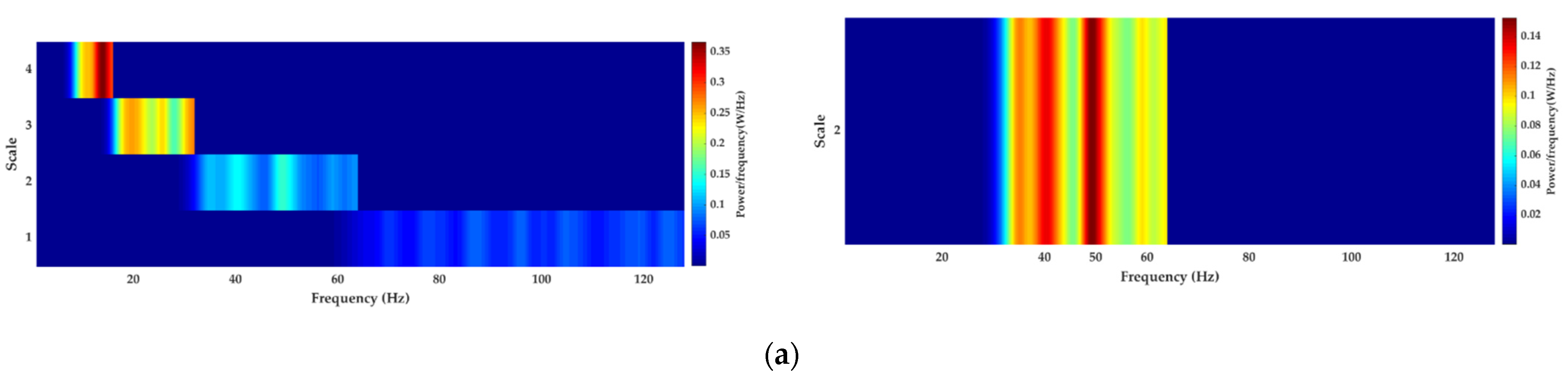
The dyadic Te-periodogram is based on the link of the detail coefficients calculated using a dyadic wavelet and the Welch–Bartlett periodogram. The use of detail coefficients in the Welch–Bartlett periodogram is due to the fact that they allow obtaining information from the analysis signal with different sensitivity. Equation (35) shows the classical Welch–Bartlett periodogram [23,30], and Equation (36) shows the dyadic Te-periodogram. The main advantage of using the detail coefficients of the different decomposition levels is that they allow obtaining a multi-sensitive fragmented frequency spectrum.
where: is the shifted signal segment , is the shifted detail coefficient segment obtained from the approximation coefficients shown in Figure 1, and are the windows of duration, and constitute the displacement distance, and .
5. Validation
5.1. Experimental Results and Discussion of Dyadic Te-Transform and Its Inverse
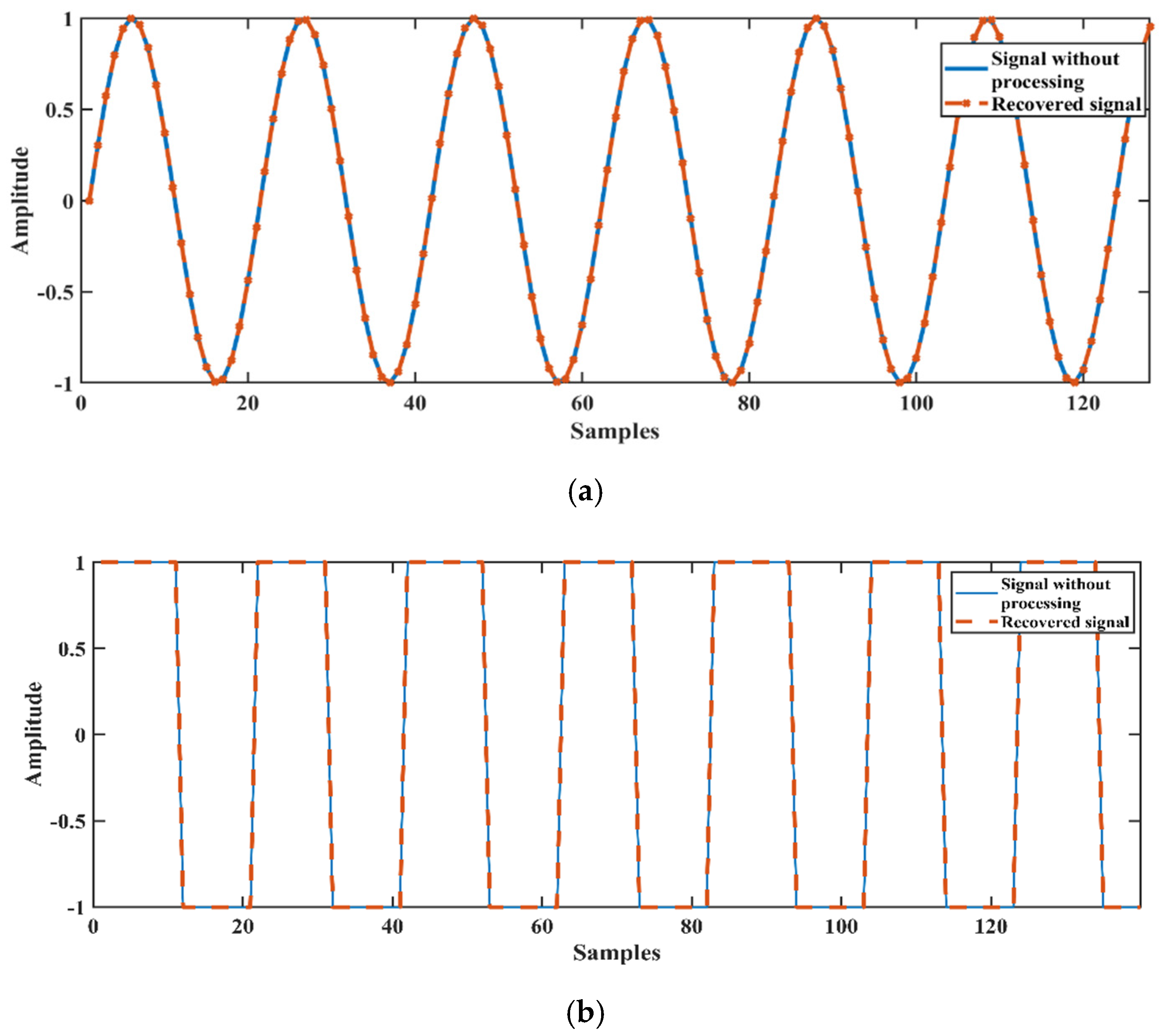
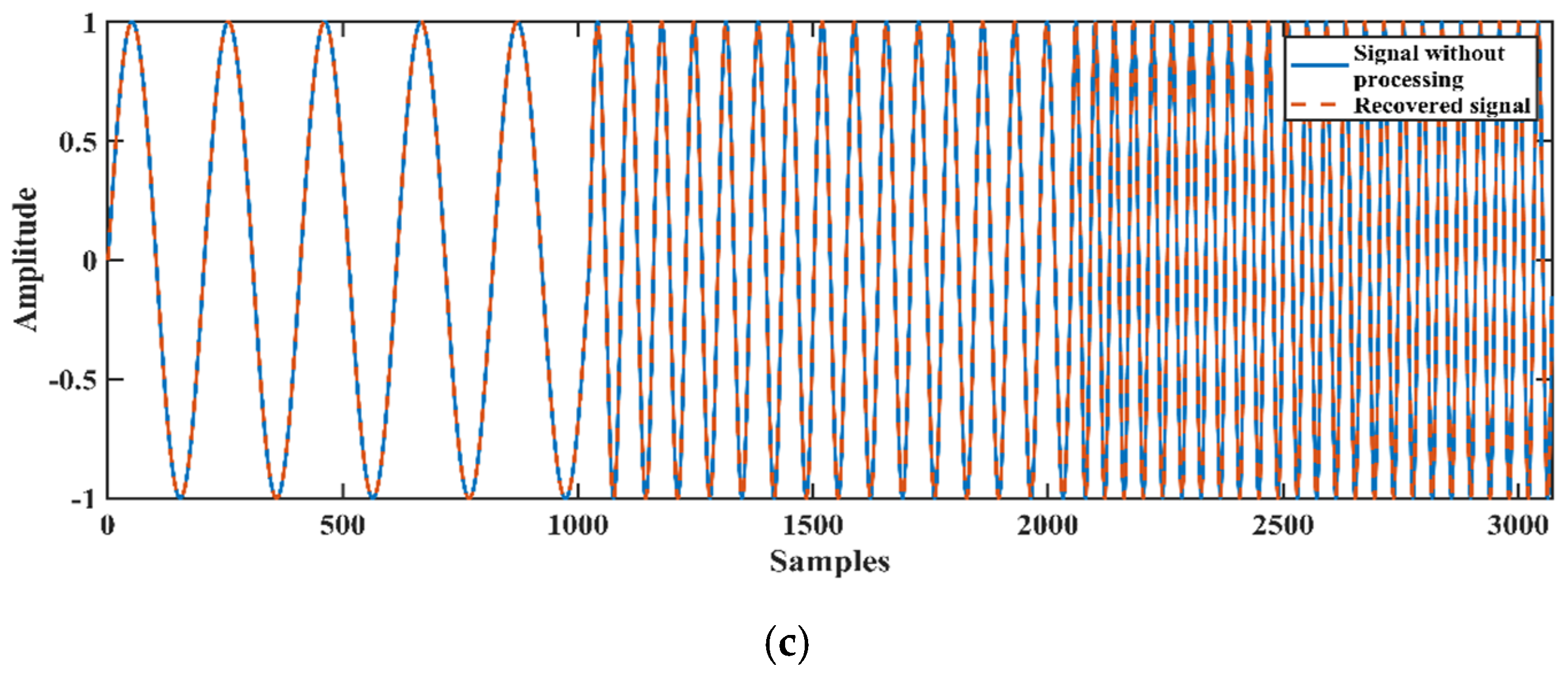
In this subsection the authors show that the dyadic Te-transform can map where , for this example, is locally and mapping . For this process, three synthetic signals were generated: the first is a sine function, the second is a pulse train, and the third is a stationary signal, see Figure 3.
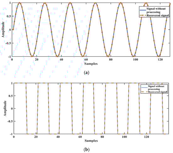
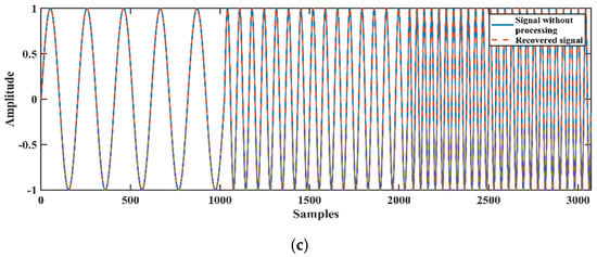
Figure 3.
Processed and recovered signals. (a) Sine function with color blue and recovered with color orange, absolute error in the recovery of . (b) Pulse train with color blue and recovered with color orange, absolute error in recovery of . (c) Non-stationary function with color blue and recovered with color orange, absolute error in the recovery of .
5.2. Analysis of a Signal in the Te Domain
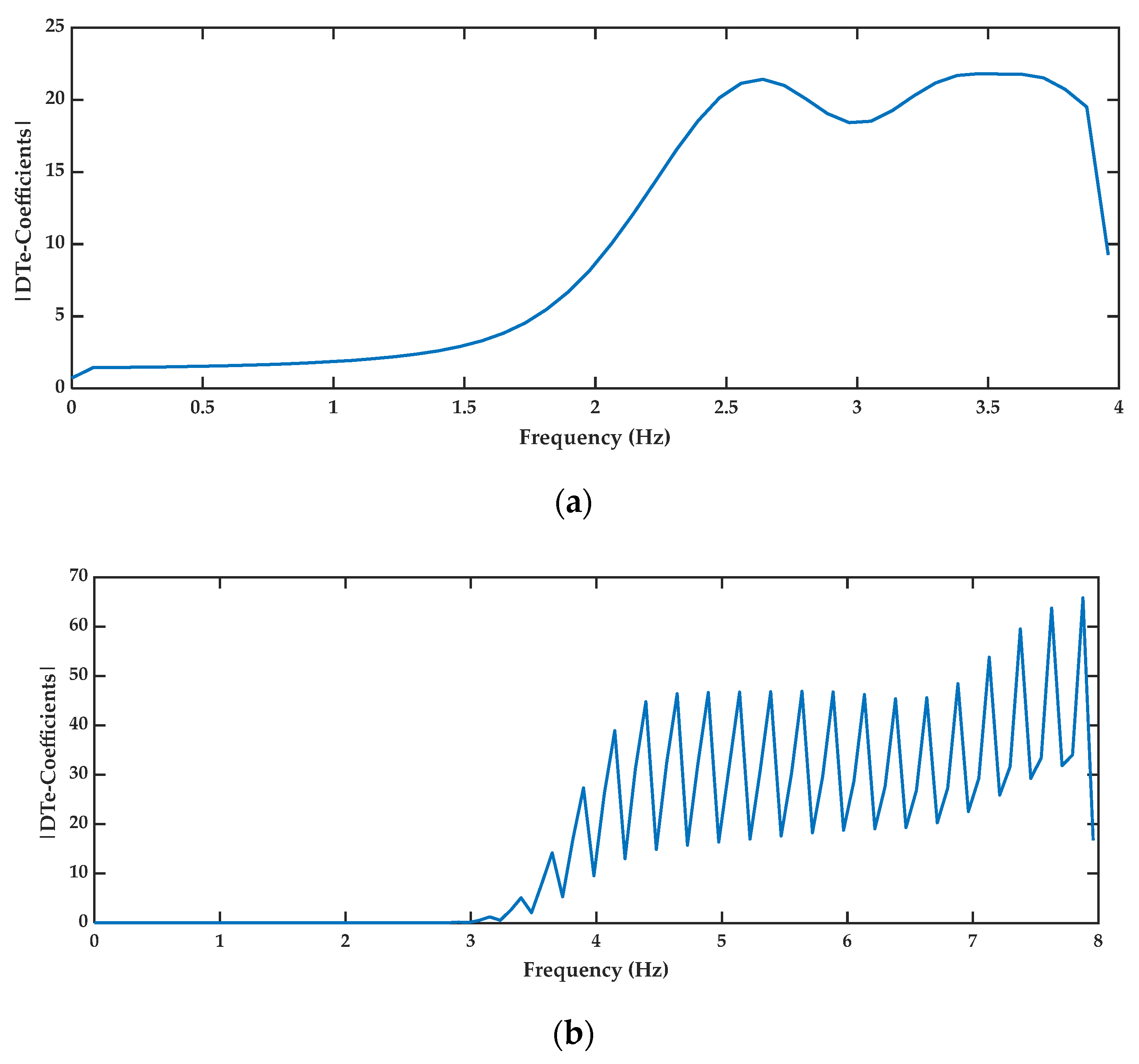
In this subsection, we analyze a non-stationary stochastic signal in the Te-domain using a Daubechies 45 wavelet function and a Kaiser-6 window. This signal has three frequency components, 15 Hz, 50 Hz, and 100 Hz, and the sampling frequency used was 256 Hz.
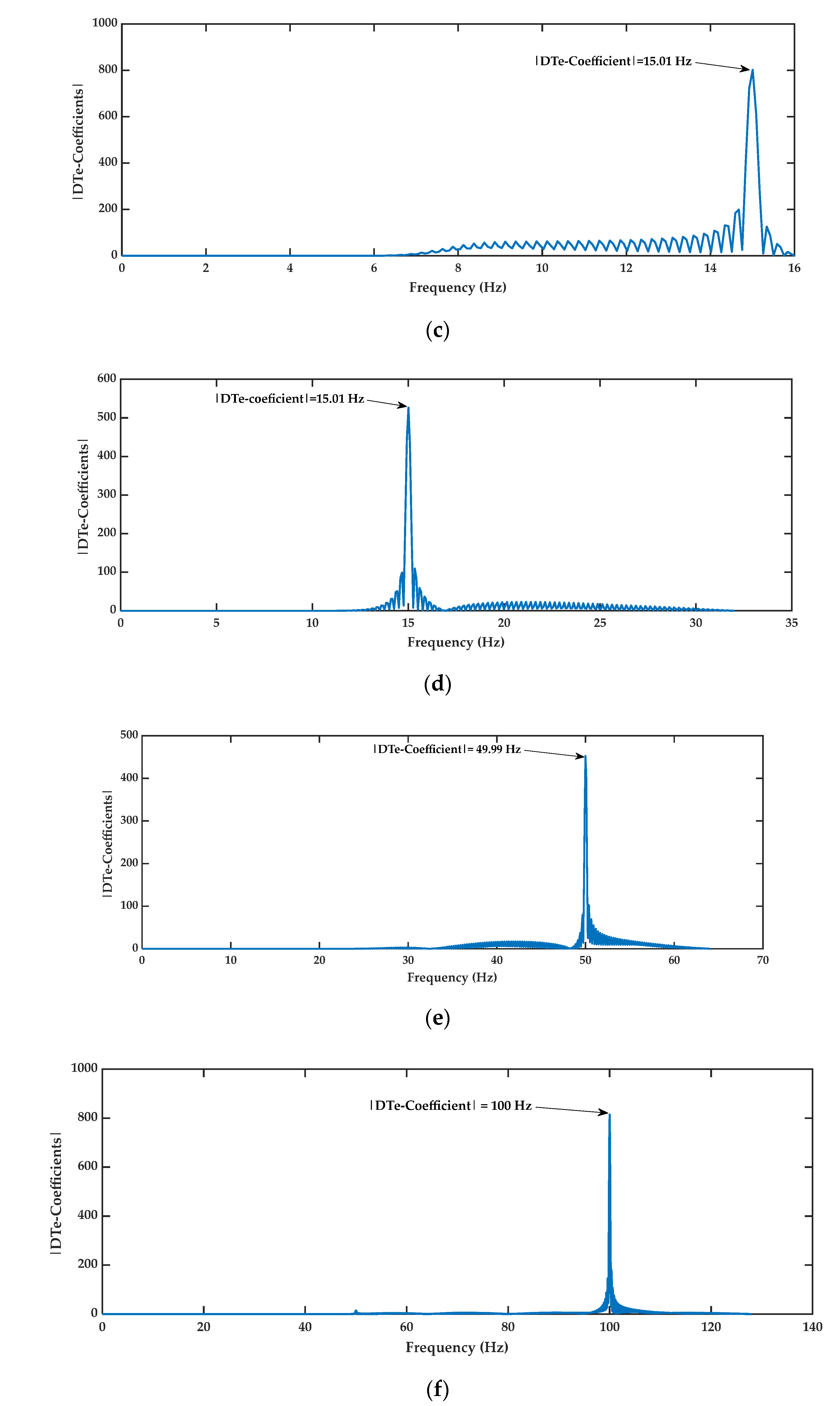
Note that in Figure 4a,b there are no frequency components. This is because the signal studied does not contain frequency components that can be extracted at decomposition levels 5 and 6. On the other hand, Figure 4c shows a frequency component of 15.01 Hz, revealing that the DTe at decomposition level 4 presents an error in the estimation of the frequency component of 0.06%.
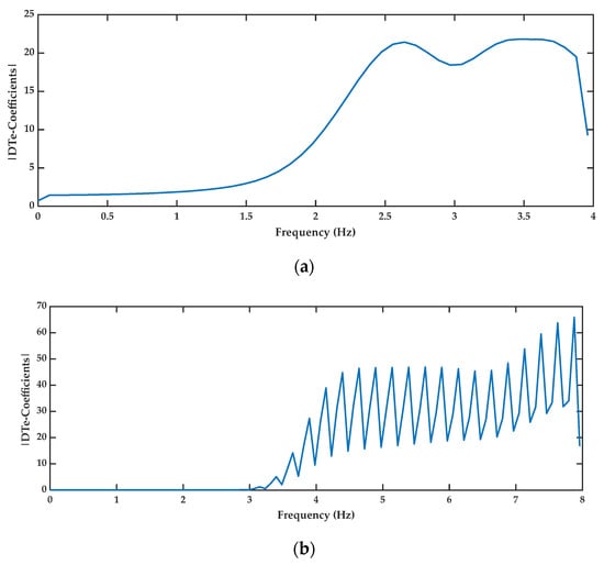
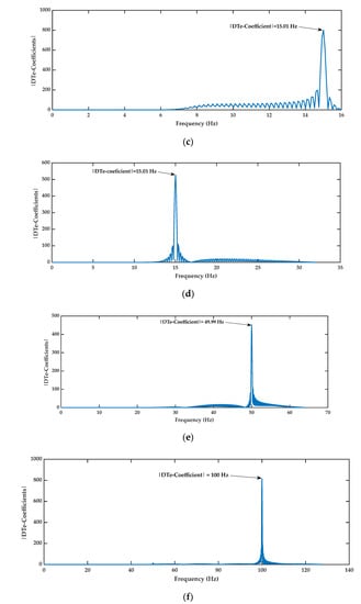
Figure 4.
Analysis of a signal in the Te domain. (a) Decomposition level 6. Estimation error N/A. (b) Decomposition level 5. Estimation error N/A. (c) Decomposition level 4. Estimation error 0.06%. (d) Decomposition level 3. Estimation error 0.06%. (e) Decomposition level 2. Estimation error 0.02%. (f) Decomposition level 1. Estimation error 0.01%.
A similar case is observed in Figure 4d because at decomposition level 3, the DTe yielded a frequency estimation error equal to decomposition level 4. Figure 4e clearly shows the frequency component close to 50 Hz with a frequency estimation error of 0.02%. Finally, Figure 4f shows the frequency component corresponding to 100 Hz showing an error in the estimation of the frequency component of 0.01%.
These results show the main advantage of DTe; they focus on the isolation of the frequency components present in a multi-component signal. The validation of the analysis performed in Section 3.3.1 shows the importance of the frequency dyadic spectrum versus cross-term attenuation.
The concept of frequency dyadic spectrum proposed in this work allows to separate the frequency components of a multi-component signal by attenuating the cross-terms.
5.3. Experimental Result and Discussion of Te-Periodogram
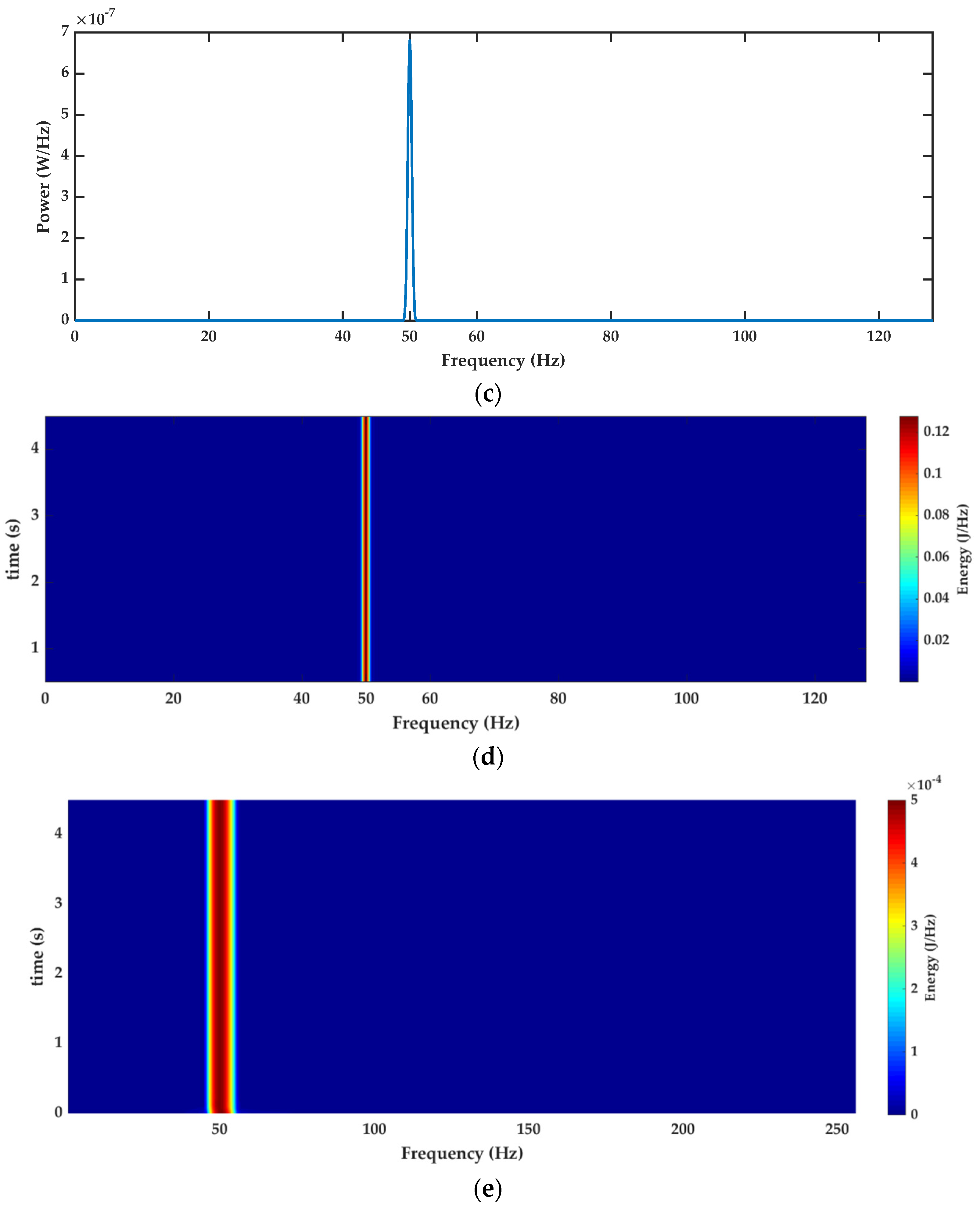
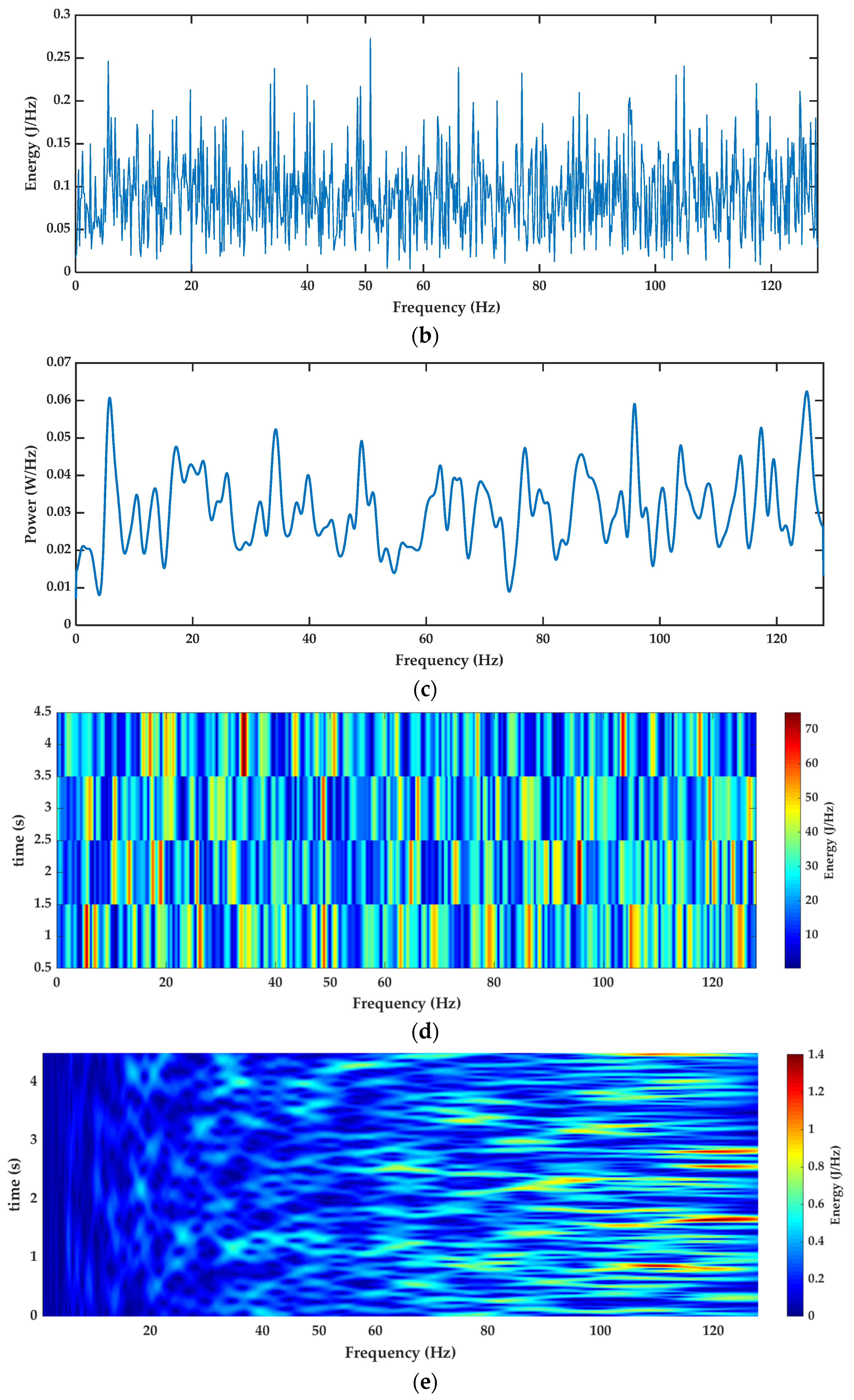
The Kaiser-6 window and the Daubechies 45 wavelet function were used to validate the dyadic Te-periodogram. Subsequently, two scenarios were generated with a synthetic signal of 50 Hz and a sampling frequency equal to 256 Hz. Once the signal was generated, we compared the Te-periodogram with other methods reported in the literature—short-time Fourier transform, Welch–Bartlett periodogram, spectrogram, and a method reported by [31]—to analyze time-frequency signals with continuous Wavelet transform (CWT). The first scenario had no noise (see Figure 5). The second scenario had a signal-to-noise ratio equal to −69 dB (see Figure 6). Note how the dyadic Te-periodogram showed excellent performance for signal-to-noise ratio equal to −69 dB, showing an error in the estimation of the frequency component of 0.8%. In the same way, the results obtained in Figure 4, Figure 5 and Figure 6 show how the frequency component can be isolated.
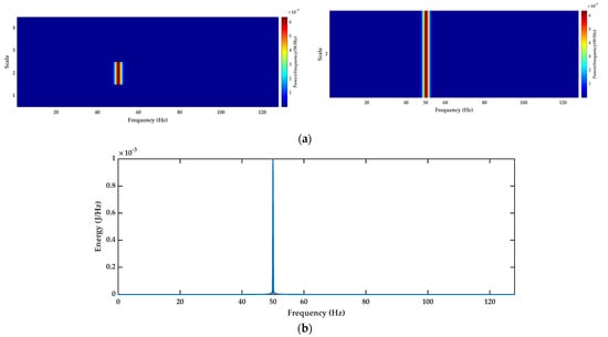

Figure 5.
Results for the first scenario (no noise). (a) Estimation error 0.06%, (b) Estimation error 0.04%, (c) Estimation error 0.02%, (d) Estimation error 0.12%, (e) Estimation error 0.2%.
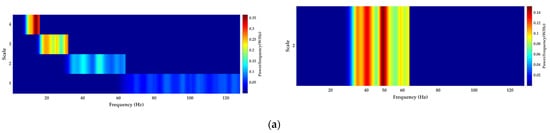

Figure 6.
Results for the second scenario (with noise). (a) Error estimation 0.8%, (b) Error estimation 1.72%, (c) Error estimation N/A, (d) Error estimation N/A, (e) Error estimation N/A.
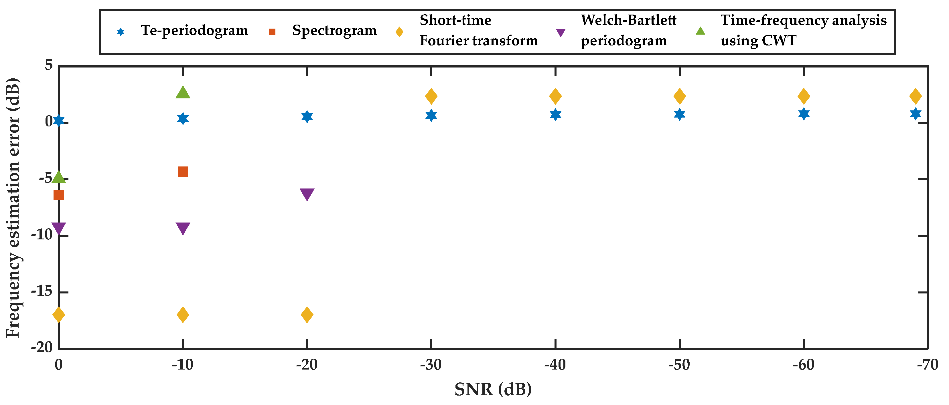
Figure 7 shows a comparison in frequency estimation error vs. SNR. The Welch–Bartlett periodogram, the spectrogram, and the method reported by [31] (time-frequency analysis using CWT) did not extract the frequency information of the signal for signal-to-noise ratios below −20 dB.
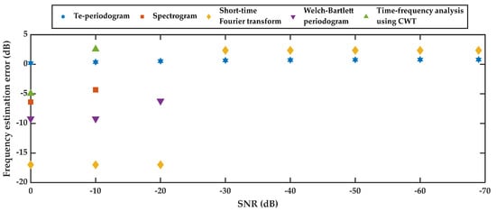
Figure 7.
Frequency estimation error.
On the other hand, note how the short-time Fourier transform was more imprecise than the Te-periodogram in the estimation of the frequency component; this result confirms the superiority of the Te-periodogram over the methods reported in the literature for the analysis of signals with signal-to-noise ratios lower than −30 dB.
6. Conclusions
The new Te-transform fulfilled the properties of the Fourier transform and the dyadic Wavelet transform. This implies that the new transform makes it possible to analyze the frequency components of a signal, but in this case in a dyadic way, allowing obtaining a dyadic frequency spectrum. Another contribution is the formulation of a corollary related to the conservation of energy in the signal before and after transforming. The main advantage that we obtain with the implementation of this methodology is that the frequency spectrum can be fragmented, obtaining multi-sensitivity, a minimum error in the recovery of the signal, and the attenuation of cross-terms. The ease that said transform provides on multi-sensitivity is observable in the new Te-periodogram since a frequency component can be detected with a signal-to-noise ratio equal to −69 dB. In future work, we will work on the analysis of the numerical stability of the dyadic Te-transform and its inverse.
Author Contributions
Conceptualization, E.T.-C.; Formal analysis, J.M.N.-J.; Supervision, D.S.-J. All authors have read and agreed to the published version of the manuscript.
Funding
This research received no external funding.
Institutional Review Board Statement
Not applicable.
Informed Consent Statement
Not applicable.
Acknowledgments
The authors thank H. Seuret-Silva for the technical support for reviewing the manuscripts. The work described in this paper is supported by CONACYT, Mexico.
Conflicts of Interest
The authors declare no conflict of interest concerning the publication of this manuscript.
References
- Meyer, Y. Wavelets: Algorithms & Applications; Society for Industrial and Applied Mathematics: Philadelphia, PA, USA, 1993. [Google Scholar]
- Goswami, J.C.; Chan, A.K. Fundamentals of Wavelets: Theory, Algorithms, and Applications; John Wiley & Sons: Hoboken, NJ, USA, 2011. [Google Scholar]
- Mallat, S. A Wavelet Tour of Signal Processing, 3rd ed.; Elsevier: Amsterdam, The Netherlands, 2009. [Google Scholar]
- Seshukumar, K.; Saravanan, R.; Suraj, M.S. Spectrum sensing review in cognitive radio. In Proceedings of the 2013 International Conference on Emerging Trends in VLSI, Embedded System, Nano Electronics and Telecommunication System, ICEVENT, Tiruvannamalai, India, 7–9 January 2013; pp. 1–4. [Google Scholar]
- Omer, A.E. Review of spectrum sensing techniques in Cognitive Radio networks. In Proceedings of the 2015 International Conference on Computing, Control, Networking, Electronics and Embedded Systems Engineering, ICCNEEE, Khartoum, Sudan, 14 January 2016; pp. 439–446. [Google Scholar]
- Goyal, D.; Pabla, B.S. The Vibration Monitoring Methods and Signal Processing Techniques for Structural Health Monitoring: A Review. Arch. Comput. Methods Eng. 2016, 23, 585–594. [Google Scholar] [CrossRef]
- Li, L.; Cai, H.; Han, H.; Jiang, Q.; Ji, H. Adaptive short-time fourier transform and synchrosqueezing transform for non-stationary Signal Separation. Signal Process. 2020, 166, 107231. [Google Scholar] [CrossRef]
- Przystupa, K.; Ambrożkiewicz, B.; Litak, G. Diagnostics of Transient States in Hydraulic Pump System with Short Time Fourier Transform. Adv. Sci. Technol. Res. J. 2020, 14, 178–183. [Google Scholar] [CrossRef]
- Zhou, S.; Xiao, M.; Bartos, P.; Filip, M.; Geng, G. Remaining Useful Life Prediction and Fault Diagnosis of Rolling Bearings Based on Short-Time Fourier Transform and Convolutional Neural Network. Shock Vib. 2020, 1–14. [Google Scholar] [CrossRef]
- Liebhart, B.; Komsiyska, L.; Endisch, C. Passive impedance spectroscopy for monitoring lithium-ion battery cells during vehicle operation. J. Power Sources 2020, 449, 227297. [Google Scholar] [CrossRef]
- KévinGuépié, B.; Grall-Maës, E.; Beauseroy, P.; Nikiforov, I.; Michel, F. Reliable leak detection in a heat exchanger of a sodium-cooled fast reactor. Ann. Nucl. Energy 2020, 142, 107357. [Google Scholar] [CrossRef]
- Wan, J.; Yao, K.; Peng, E.; Cao, Y.; U, Y.N.I.; Yu, J. Separation characteristics between time domain and frequency domain of wireless power communication signal in wind farm. EURASIP J. Wirel. Commun. Netw. 2020, 2020, 1–12. [Google Scholar] [CrossRef]
- Pham, M.T.; Kim, J.M.; Kim, C.H. Accurate bearing fault diagnosis under variable shaft speed using convolutional neural networks and vibration spectrogram. Appl. Sci. 2020, 10, 6385. [Google Scholar] [CrossRef]
- Manhertz, G.; Bereczky, A. STFT spectrogram based hybrid evaluation method for rotating machine transient vibration analysis. Mech. Syst. Signal Process. 2021, 154, 107583. [Google Scholar] [CrossRef]
- Tran, T.; Lundgren, J. Drill Fault Diagnosis Based on the Scalogram and Mel Spectrogram of Sound Signals Using Artificial Intelligence. IEEE Access 2020, 8, 203655–203666. [Google Scholar] [CrossRef]
- Sahoo, S.; Das, J.K. Application of Adaptive Wavelet Transform for Gear Fault Diagnosis Using Modified-LLMS Based Filtered Vibration Signal. Recent Adv. Electr. Electron. Eng. 2018, 12, 257–262. [Google Scholar] [CrossRef]
- Maher, P.; Young, N. An Introduction to Hilbert Space; Cambridge University Press: Cambridge, UK, 1991. [Google Scholar]
- Cooley, J.W.; Lewis, P.A.W.; Welch, P.D. The Fast Fourier Transform and Its Applications; Prentice-Hall, Inc.: Hoboken, NJ, USA, 1969. [Google Scholar]
- Napolitano, A. Cyclostationary Processes and Time Series: Theory, Applications, and Generalizations; Academic Press: London, UK, 2019. [Google Scholar]
- Hong, D.; Wang, J.; Gardner, R. Real Analysis with an Introduction to Wavelets and Applications; Elsevier: Amsterdam, The Netherlands, 2004. [Google Scholar]
- Griffel, D.H.; Daubechies, I. Ten Lectures on Wavelets; Siam: Philadelphia, PA, USA, 1995. [Google Scholar]
- Gao, R.X.; Yan, R. Wavelets: Theory and Applications for Manufacturing; Springer Science & Business Media: Berlin, Germany, 2011. [Google Scholar]
- Manolakis, D.; Ingle, V.; Kogon, S. Statistical and Adaptive Signal Processing: Spectral Estimation, Signal Modeling, Adaptive Filtering, and Array Processing; McGraw-Hill: Boston, MA, USA, 2005. [Google Scholar]
- Shah, F.A.; Debnath, L. Wavelet neural network model for yield spread forecasting. Mathematics 2017, 5, 72. [Google Scholar] [CrossRef] [Green Version]
- Bakić, D.; Krishtal, I.; Wilson, E.N. Parseval frame wavelets with En(2)-dilations. Appl. Comput. Harmon. Anal. 2005, 19, 386–431. [Google Scholar] [CrossRef] [Green Version]
- Luthy, P.M.; Weiss, G.L.; Wilson, E.N. Projections and dyadic Parseval frame MRA wavelets. Appl. Comput. Harmon. Anal. 2015, 39, 511–533. [Google Scholar] [CrossRef]
- Li, Z.; Shi, X. Parseval frame wavelet multipliers in L2(ℝd). Chin. Ann. Math. Ser. B 2012, 33, 949–960. [Google Scholar] [CrossRef]
- Kadambe, S.; Boudreaux-Bartels, G.F. A Comparison of the Existence of “Cross Terms” in the Wigner Distribution and the Squared Magnitude of the Wavelet Transform and the Short Time Fourier Transform. IEEE Trans. Signal Process. 1992, 40, 2498–2517. [Google Scholar] [CrossRef]
- Pachori, R.B.; Sircar, P. A novel technique to reduce cross terms in the squared magnitude of the wavelet transform and the short-time Fourier transform. In Proceedings of the 2005 IEEE International Workshop on Intelligent Signal Processing, Faro, Portugal, 1–3 September 2005; pp. 217–222. [Google Scholar]
- Proakis, J.G.; Monolakis, D.G. Digital Signal Processing: Principles, Algorithms, and Applications; Pearson Education: New Delhi, India, 1996. [Google Scholar]
- Nuñez, M. Time Frequency Analysis Using CWT. MATLAB Central File Exchange. Retrieved 11 November 2021. Available online: https://www.mathworks.com/matlabcentral/fileexchange/64860-time-frequency-analysis-using-cwt (accessed on 25 July 2021).

Publisher’s Note: MDPI stays neutral with regard to jurisdictional claims in published maps and institutional affiliations. |
© 2021 by the authors. Licensee MDPI, Basel, Switzerland. This article is an open access article distributed under the terms and conditions of the Creative Commons Attribution (CC BY) license (https://creativecommons.org/licenses/by/4.0/).