1. Introduction
The theory of fractional integrals and derivatives of arbitrary real or complex orders dates back approximately three centuries. In recent years, researchers have shown that differential equations with non-integer order derivatives can better model real-world physical phenomena than integer-order derivatives. Because of their importance in science and engineering, chemistry, physics, finance, and other fields [
1], fractional differential equations have received increasing attention in recent years. In some cases, the analytical solution to fractional differential equations can be obtained using Laplace and Fourier transforms, as well as the Green function [
2,
3]. Due to the presence of a singular kernel in fractional derivatives, it is difficult to find an analytical solution for the majority of fractional differential equations.
In this paper, we implement a difference analog of the Caputo fractional derivative known as the
[
4] formula, which provides second-order global convergence in the time direction. Abbaszadeh and Dehghan [
5] developed an accurate and robust numerical solution for solving neutral delay time-space distributed-order fractional damped diffusion-wave equation based on the Galerkin meshless method. They also obtained a meshless numerical simulation for a fractional damped diffusion-wave equation with delay [
6]. Abbaszadeh et al. [
7] introduced an interpolating stabilized element-free Galerkin method for neutral delay fractional damped diffusion-wave equations. In some important applications, the fourth-order derivative term plays a crucial role. Nikan et al. [
8] proposed an efficient numerical procedure, the local radial basis function created by the finite difference method, for computing the approximation solution of the time-fractional fourth-order reaction-diffusion equation in terms of the Riemann–Liouville derivative. The time-fractional derivative was estimated using the second-order accurate formulation, while the spatial terms were discretized using the local radial basis function generated by the finite difference method. Huang and Stynes [
9] studied
-robust error analysis of a mixed
-finite element method for a time-fractional fourth-order diffusion equation. For a two-dimensional distributed-order time-fractional fourth-order partial differential equation, Fakhar-Izadi [
10] investigated the space-time Petrov–Galerkin spectral approach. The problem is converted to a multi-term time-fractional equation by using an appropriate Gauss-quadrature rule to discretize the distributed integral operator. Liu et al. [
11] presented and discussed a finite difference/finite element algorithm for casting about for numerical solutions to a time-fractional fourth-order reaction–diffusion problem with a nonlinear reaction term, which is based on a finite difference approximation in time and a finite element method in spatial direction. Moreover, many numerical methods have been developed for solving different classes of fractional differential equations such as spectral methods [
12,
13,
14,
15,
16,
17,
18,
19], finite difference methods [
20,
21,
22,
23,
24,
25], finite element methods [
26,
27], finite volume method [
28,
29], and matrix transfer technique [
30,
31]. The study of delay differential equations with fractional derivatives is rapidly expanding these days since they are frequently employed in modeling of elastic media and stress–strain behavior for the torsional model, control difficulties, high-speed machining communications, and so on [
1].
The multidimensional fourth order nonlinear fractional subdiffusion model with time delay is obtained from the standard problem by replacing the first-order time derivative by fractional derivatives in the Caputo sense. The analytical solution of this problem is only gained for the linear case when the coefficients constants. Recently, the authors of [
32,
33,
34] constructed numerical techniques for this problem with fourth-order fractional diffusion wave equations and some modifications have been considered in [
35]. In [
36], a Newton-linearized compact ADI scheme for Riesz space fractional nonlinear reaction-diffusion equations was constructed and analyzed. The numerical computation for a class of fourth-order linear fractional subdiffusion equations with spatially variable coefficient under the first Dirichlet boundary conditions were considered in [
37]. Two finite difference schemes with second-order accuracy were derived by applying
formula and
formula, respectively, to approximate the time Caputo derivative. Liu et al. [
38] studied and analyzed a Galerkin mixed finite element method combined with time second-order discrete scheme for solving nonlinear time fractional diffusion equation with fourth-order derivative term. Most of the numerical techniques opted in the articles are based upon
approximation of Caputo time derivative which gives first-order convergence for fractional order
, where
is the fractional order (present in time-fractional derivative). Recently, articles based on orthogonal spline collocation method are published [
39] which focus on weakly singular solutions and constructing a high-order numerical scheme for fourth-order subdiffusion equations.
In the real world, parameters such as the coefficients in the problem under consideration are spatially or temporally variable. Therefore, presenting a numerical scheme and finding numerical solution becomes a tedious task. There are many difficulties to build numerical schemes for fourth-order fractional differential equations with delay due to non-locality of the problem, variable coefficients, nonlinearity, and error depends upon the history of considered problem. Therefore, the main issue we address in this paper is introducing an effective numerical approach for multi-dimensional fourth-order fractional subdiffusion equations with delay. In the studies discussed above and mainly in literature, there is a lack of studies available on delay differential equations.
In this paper, our target is to present high ordered difference scheme to solve the following two-dimensional time-fractional subdiffusion equation of fourth-order with variable coefficients and nonlinear source term having a delay constant.
with the initial and the boundary conditions:
where
and
is its boundary. Here,
is the temporal Caputo fractional operator of order
,
is the constant delay parameter and
is the nonlinear source function with delay.
,
,
,
,
,
,
,
, and
are all given sufficiently smooth functions. Now, we present the definitions of fractional integral, and fractional derivatives which would be used later.
Definition 1. The Caputo fractional derivative [40] of order is defined by Next, for discretization, we partition the mesh , where , , . Introducing the positive integers , , and N, let , , ( is a positive constant) are the spatial and temporal steps respectively. Define , , , , , .
1.1. The Discretization of the Time Fractional Operator
Alikhanov [
4] constructed a discrete approximation for Caputo fractional derivative which will be mentioned firstly. Next, some Lemmas important in the later context are introduced to aid in constructing the numerical scheme for the system (1).
Definition 1 ([
4]).
Let , the approximated formula for at the fixed point , , is called formula of second order temporal convergence for , given as follows:Let , , ,
, ,
For , , and
further when ,Defining Below given Lemma estimates the error of the formula.
Lemma 1 ([
4]).
For any and , it holds that The next lemmas are giving some technical properties for Alikhanov formula.
Lemma 2 ([
41,
42]).
Let function , , and , then For any
,
,
, we introduce the following notations:
Now, we define inner products and discrete norms useful in the analysis section of the described numerical scheme (for any
):
1.2. Numerical Scheme Construction
A numerical scheme is constructed by employing the linear operator for the spatial dimensions and the approximation of Caputo time-fractional derivative.
Substituting (
7) into (1a), yields
The numerical scheme for (1) is ready after that order reduction. Considering Equations (
8)–(
10) at
yields
Using Lemma 1, we can write
Using the Taylor’s expansion we can write the following equalities:
Acting the operator
on (
16) gives
Similarly, acting the operator
on (
17) gives
Employing Taylor’s expansion for the source term (linearization) gives
Acting the operator
on Equations (
11)–(
13) and substituting above equations gives
where
,
,
,
,
, , , ,
, , , , and there exists a positive constant C such that , , , .
Noticing the initial and boundary conditions at
Omitting the small terms in (
21)–(
23), we construct the numerical scheme for (1) as follows:
such that
2. Numerical Simulations
Two examples are presented here to show the efficiency of numerical scheme (29) for the problem defined in (1). Let be the solution of proposed numerical scheme.
Denote . , , .
Example 1. Consider the following two-dimensional fourth-order subdiffusion equation:
where the initial and boundary conditions are defined specially so that the exact solution of above problem is Problem (1) is solved using our proposed method. The numerical results are listed in
Table 1 and
Table 2. It can be monitored from the results that our proposed method gives
order of convergences. The numerical results are obtained for different values of fractional order
with varying values of time and spatial step sizes.
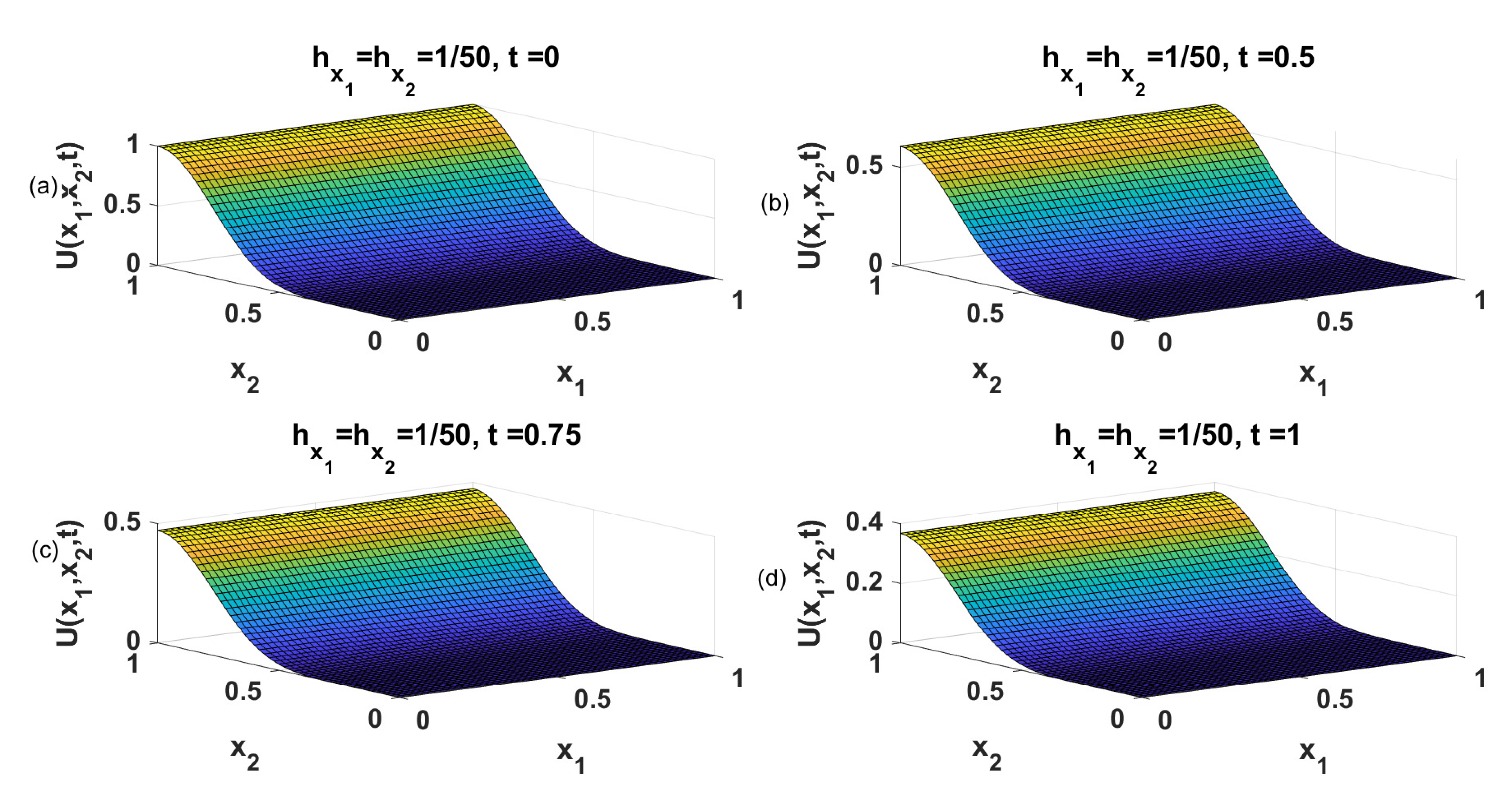
Figure 1 gives surface plot for different values of time
. The variation in numerical values can be observed from the varying range in
with respect to change in the value of time variable. The obtained convergence orders are approximately 4, 4, 2 for spatial directions and time direction, respectively, and same is validated in Stability and Convergence section discussed above.
We present a second problem solved with described numerical scheme. Maximum error was being computed for varying step sizes in space and time dimensions as given in
Table 3 and
Table 4. The decrease in error can be observed from these tables with decrease in step size. Moreover, we can observe that approximate convergence orders for space and time are 4 and 2, respectively.
Figure 2 depicts the numerical solution for different values of time variable with spatial step sizes
. Moreover, the convergence orders for spatial and time dimensions are authenticated in Stability and convergence section as well.
Example 2. Consider the two dimensional fourth order subdiffusion equation in the following form:
The exact solution of above example is 2.1. A Final Example
Finally, we consider a problem whose exact solution is not known to us.
Similar to above problems, we find the numerical results using the numerical scheme given in Equation (29). The above problem has variable coefficients and the exact solution is not known to us; therefore, we check the accuracy of proposed numerical scheme by means of absolute residual error function, which is a measure of how well the approximation satisfies the original nonlinear fractional differential problem given in Example
Section 2.1. The absolute residual error is defined as
The numerical results are shown in
Figure 3 with different time variable values.
Table 5 and
Table 6 show the numerical results of residual error
,
. From our numerical results, we can conclude that numerical and theoretical results are in agreement. The numerical scheme gives the global second-order time convergence and fourth-order convergence in spatial dimensions. The accuracy of getting convergence order becomes more pronounced when step sizes are decreased. In all the calculations MATLAB is used.


