F4: An All-Purpose Tool for Multivariate Time Series Classification

Abstract

We propose Fast Forest of Flexible Features (F4), a novel approach for classifying multivariate time series, which is aimed to discriminate between underlying generating processes. This goal has barely been addressed in the literature. F4 consists of two steps. First, a set of features based on the quantile cross-spectral density and the maximum overlap discrete wavelet transform are extracted from each series. Second, a random forest is fed with the extracted features. An extensive simulation study shows that F4 outperforms some powerful classifiers in a wide variety of situations, including stationary and nonstationary series. The proposed method is also capable of successfully discriminating between electrocardiogram (ECG) signals of healthy subjects and those with myocardial infarction condition. Additionally, despite lacking shape-based information, F4 attains state-of-the-art results in some datasets of the University of East Anglia (UEA) multivariate time series classification archive.

1. Introduction

Time series classification (TSC) is a hot topic with applications in many fields, including economics, finance, environmental sciences, medicine, physics, speech recognition and multimedia, among many others. Given a set of univariate (UTS) or multivariate (MTS) time series with class labels, the target is to train an algorithm to predict the class of unlabelled time series. Unlike UTS, MTS involve a number of variables or dimensions which should be jointly considered to extract information about its right class label. Although many algorithms have been developed in the last few years for univariate time series classification (UTSC), multivariate time series classification (MTSC) has received much less attention (a review on the topic of feature-based MTSC can be seen in [1]). However, the increasing amount of data that are generated every day by sensors and Internet of Things (IoT) devices makes totally pivotal the development of fast and accurate MTSC algorithms. For instance, it is common for doctors to decide whether or not a patient is likely to suffer a myocardial infarction based on multivariate ECG data. The availability of MTSC approaches capable of tackling this task in an automated manner could free healthcare professionals from individually examining each ECG, resulting in increased efficiency. Similar examples can be extracted from different application fields. In [2], a comprehensive overview on MTSC, including current advances, future prospects, important references and several application areas, is provided.

One of the first approaches for MTSC was introduced in the early work [3]. Each MTS is characterised by means of a set of spectral matrices and then a classifier based on measures of divergence between the corresponding sets is proposed. By nature, this approach is aimed at classifying MTS according to the underlying multivariate process. However, in [3], the procedure is only assessed with a real dataset of MTS coming either from earthquakes or explosions without reporting the results of its behaviour for different generating models.

Some approaches for MTSC based on dimensionality reduction techniques were introduced in the last decade [4,5,6]. In [4,5], two different procedures of feature selection for MTS using the singular value decomposition (SVD) were proposed. The first approach considers the first singular vector, whereas the second one considers the first two dominating singular vectors weighted by their associated singular values. The correlations between dimensions are taken into account in both cases, but the class labels are ignored when the feature extraction is performed. To address this issue, Weng and Xen [6] proposed to classify MTS by using locality preserving projections (LPP). The method consists of two steps. First, feature extraction is carried out by using one of the approaches in [4] or [5]. Second, the feature vectors are projected in a lower dimensional space in a way that MTS sharing the same class label are close to each other. In the reported simulation study, Weng and Xen [6] also considered the two-dimensional singular value decomposition (2dSVD) for MTSC, which was introduced in [7] as an extension of the classical SVD to sets of 2D objects, as matrices.

A classical technique to perform TSC is based on the dynamic time warping (DTW) distance along with the one nearest neighbour (1NN) classifier (see, e.g., [8,9]). Two main extensions of this distance are frequently used in MTSC tasks [10]. Furthermore, multivariate DTW has been used along with other distances to develop some sophisticated MTSC procedures. In this regard, Mei et al. [11] proposed an approach considering DTW and the Mahalanobis distance. Bankó and Abonyi [12] presented a novel algorithm called correlation based dynamic time warping where DTW and PCA-based similarity measures are combined so that the correlation between dimensions is taken into consideration in the classification procedure. Górecki and Luczak [13] introduced a method called derivative dynamic time warping where the distance between two MTS is defined as a convex combination of the multivariate DTW distances between them and between their derivatives. A hyperparameter $\alpha$ chosen in the learning phase (by leave-one-out cross-validation) determines the weight of each individual distance and the 1NN rule is used to classify new observations. The procedure is shown to improve the results achieved by DTW in some datasets. Due to their generally great performance on classifying MTS, the multivariate extensions of DTW distance with the 1NN classifier are usually considered as a benchmark when a new MTS classification approach is introduced [11,14,15,16]. Indeed, in [14], where an extensive analysis of some of the most promising approaches for MTSC is performed, the authors conclude that: The standard TSC benchmark, DTW, is still hard to beat and competitive with more recently proposed alternatives.

Approaches based on word extraction and symbolic representations have also been constructed for MTSC. Schäfer and Leser [16] proposed WEASEL+MUSE, which builds a multivariate feature vector, first using a sliding window approach applied to each UTS constituting the MTS and then extracting the discrete features by window and dimension. Next, the feature vector is utilised in a traditional classifier. WEASEL+MUSE is based on the WEASEL classifier that the same authors proposed for UTS relying on a similar idea [17]. Baydogan and Runger [18] introduced a classifier based on a new symbolic representation, called SMTS, where all the dimensions are simultaneously considered. The procedure builds on the application of two random forests, one for variable selection and the other for the classification task.

The well-known idea of ensemble learning has also played a central role in MTSC in recent years. The most successful method considering this approach is the Hierarchical Vote Collective of Transformation-based Ensembles, so-called HIVE-COTE, which combines classifiers based on five types of discriminatory features. Although it was originally designed for UTSC [19], a multivariate extension can easily be developed by building each component as an independent ensemble [14]. Multivariate HIVE-COTE is, on average, one of the best performing algorithms when dealing with the datasets contained in the University of East Anglia (UEA) multivariate time series classification archive [20].

Deep learning algorithms have also been applied to MTSC during the last few years. Karim et al. [15] proposed a long short-term memory fully convolutional network (LSTM-FCN) to perform the classification task. This work is an extension of a previous work where a fully convolutional with long short-term memory recurrent neural network is introduced to perform UTSC [21]. The results given in [15] indicate that the LSTM-FCN beats the state of the art in many of the considered datasets. However, it is worth mentioning that these results differ from the ones reported in [14], where LSTM-FCN was tested in some of the same datasets. As it is stated there: The deep learning algorithms have been disappointing in these experiments. They have a tendency to occasionally completely fail. No doubt these will be improved over time, but, as yet, they are not consistently state-of-the-art. This casts doubt on the ability of the current deep learning techniques to solve MTSC problems. Liu, Hsaio and Tu [22] designed a methodology for MTSC relying on convolutional neural networks (CNN). The approach is based on a tensor scheme along with an innovative deep learning architecture considering multivariate and lag-feature characteristics. Fan, Shrestha and Qiu [23] presented a technique to classify spatial temporal patterns which employs spiking neural networks (SNN). The method is evaluated in some MTS datasets, achieving a performance comparable to deep neural networks.

There also exists some methods based solely on statistical feature extraction and then on feeding a traditional classifier with the extracted features. For example, Zagorecki [24] developed a generic method which extracts many statistical quantities from a given MTS. The majority of those are derived from each UTS individually, but the approach also considers the cross-correlation between each pair of UTS, thus accounting for the relationship between dimensions. This method was the runner-up in the 2015 AAIA Data Mining Competition [25], in which 80 participant teams took part, thus proving itself as a powerful approach.

The above-mentioned MTSC methods are fairly general in the sense that they are presented to be applied to an arbitrary MTS dataset. A few other proposed approaches are domain-specific. In [26], an approach particularly designed to classify multivariate ECG data is provided. The method performs feature extraction via the maximum overlap discrete wavelet transform (MODWT), and the features are then used to feed a linear or quadratic discriminant analysis classifier. The approach is shown to compare favourably with other techniques for classifying ECG signals. Formisano, De Martino and Valente [27] designed a straightforward approach to classify multivariate functional magnetic resonance imaging (fMRI) signals involving two steps: feature selection based on raw fMRI data through recursive feature elimination, and application of a support vector machine considering the selected features. Seto, Zhang and Zhou [28] presented a technique for classifying MTS from human activity recognition. It first builds a paragon for each class by using cluster analysis in the training data. Then, feature extraction is performed via DTW and a classifier, such as the support vector machine, is applied.

Aside from [3,26], all the mentioned approaches address the MTSC task from a shape-based point of view, in the sense that they assume that MTS in different classes are mainly characterised by different geometric profiles. It seems surprising that, in the last 20 years, almost nobody has proposed a procedure for classifying MTS in a setting where the different categories are associated with distinct underlying generating processes. Furthermore, although the approaches in [3,26] should be able to distinguish between generating processes, their performance is only illustrated with real datasets in those works. Thus, their effectiveness under different dependence structures between classes has not been examined. To the best of our knowledge, none of the existing MTSC approaches have been evaluated in a scenario with different multivariate generating processes. However, such a situation is not uncommon. For instance, it is well known that the MTS of daily returns of different pairs of sector indexes can be modelled by means of multivariate generalized autoregressive conditional heteroscedasticity (MGARCH) models with different coefficients [29]. Furthermore, multivariate electroencephalogram (EEG) signals collected from a group of subjects have been shown to follow vector autoregressive moving average (VARMA) models whose coefficients depend on the specific mental task that the subject is performing [30].

In addition, due to the lack of methods addressing the MTSC task from the previously stated point of view, it remains uncertain if a classifier of this nature would do a good job when dealing with the real datasets most commonly considered in MTSC, for example, the ones included in the UEA multivariate time series classification archive. The archive consists of 30 MTS datasets covering a wide range of cases, dimensions and series lengths. Some approaches such as multivariate DTW, WEASEL + MUSE and HIVE-COTE have been tested with these datasets, showing a great performance. However, it remains totally unanswered if the different classes in these datasets, or at least in some of them, can be described by means of the underlying dependence structures in addition to the shapes. If so, the implications of this fact would be profound, as it would encourage researchers to take into account dependence measures when coping with a MTSC task.

The first contribution of this paper is to introduce a novel approach for classifying MTS aimed at discriminating between underlying generating processes. The proposed classifier is based on the quantile cross-spectral density (QCD) and the maximum overlap discrete wavelet transform (MODWT). Both spectral tools are utilised to extract suitable features, which are then used to feed a random forest classifier. Consideration of QCD and MODWT is motivated by our previous work [31], where they separately proved their usefulness in MTS clustering, exhibiting a high discriminatory power. Unlike other conventional spectral features, quantile cross-spectral densities examine the dependence between the components in quantiles, thus allowing us to simultaneously characterise cross-sectional and serial dependence, exhibiting robustness to outliers and heavy tails and capturing changes in the conditional shape (skewness, kurtosis). On the other hand, the wavelet features are useful to distinguish between signals with spectra changing over time and hence particularly suitable to deal with nonstationary processes. Therefore, both feature types provide a valuable picture of the underlying dynamic structures and report complementary information so that their combined use is expected to increase the classification accuracy. Our approach avoids the need to analyse and model each single MTS, which is computationally expensive and far from being the actual goal. The second contribution of this work is to show how the proposed methodology can be successfully applied to discriminate between ECG signals of healthy subjects and those with myocardial infarction condition, which is an active and important research topic. Finally, the third contribution is to show the excellent results reached by the proposed approach in some classical MTS datasets despite lacking shape-based information.

The remainder of this paper is organised as follows. In Section 2, we present the proposed classifier along with some related theoretical background and a toy example illustrating its usefulness. Section 3 shows an extensive assessment of the proposed approach via a simulation study covering a broad variety of scenarios. The corresponding classes are represented by means of different stationary processes. The proposed classifier is compared with some competitive alternatives reported in the literature. In Section 4, the classifier is evaluated in nonstationary settings. The effectiveness of the method and its competitors when varying the amount of training data and the series length is reported in Section 5. The computation times of the analysed procedures are discussed through Section 6. Section 7 illustrates the application of the proposed methodology to a classical dataset containing ECG data. In Section 8, the classification method is applied to some datasets in the UEA archive. Some concluding remarks and future work are provided in Section 9.

2. A Combined Feature-Based Approach for Multivariate Time Series Classification

In this section, we present Fast Forest of Flexible Features (F4), the proposed approach for classifying MTS. After some brief comments on the considered features and some theoretical background, the classifier F4 is introduced and a motivating example is used to highlight the advantages of combining the selected features.

2.1. Combining Two Types of Features

F4 is based on a combination of two types of features. In [31], we proposed a dissimilarity measure based on QCD to perform clustering of MTS, so-called $d_{QCD}$. In an extensive simulation study where a range of state-of-the-art dissimilarities were compared, $d_{QCD}$ turned out to be the average best-performing measure, showing robustness against the generating mechanism and exhibiting low computation times. On the other hand, a dissimilarity based on multiple-scale wavelet variances and wavelet correlations, so-called $d_W$ [32] also worked very well in the majority of scenarios simulated in [31], besides being the most efficient. Both $d_{QCD}$ and $d_W$ are simply Euclidean distances between extracted features and their high capability to discern between generating processes in an unsupervised learning context suggests great performance when facing supervised classification tasks. Furthermore, given their different nature, it is expected that a classifier considering both types of features significantly improves the behaviour of classifiers based on only one of these features. Whereas $d_{QCD}$ focuses on capturing the dependence structure at different pairs of quantile levels, $d_W$ relies on decomposing a signal into a set of mutually orthogonal wavelet basis functions. Both features complement each other, with $d_{QCD}$ well suited to detect different dependence structures in parts of the joint distribution (which remain hidden for standard spectral measures), and $d_W$ relying on a time-frequency analysis which allows us to capture differences in times where the changes occur, and hence particularly useful to deal with series exhibiting long-range dependence and nonstationarity.

2.2. Background

Some background knowledge of QCD and MODWT is provided below.

2.2.1. The Quantile Cross-Spectral Density

Following [31], let $\{{\mathbf{X}}_t,t\in \mathbb{Z}\}=\{(X_{t,1},\dots ,X_{t,d}),t\in \mathbb{Z}\}$ be a d-variate real-valued strictly stationary stochastic process. Denote by $F_j$ the marginal distribution function of $X_{t,j}$, $j=1,\dots ,d$, and by $q_j\left(\tau \right)=F_j^{-1}\left(\tau \right)$, $\tau \in [0,1]$, the corresponding quantile function. Fixed $l\in \mathbb{Z}$ and an arbitrary couple of quantile levels $(\tau ,{\tau }^{\prime })\in {[0,1]}^2$, consider the cross-covariance of the indicator functions $I\{X_{t,j_1}\le q_{j_1}\left(\tau \right)\}$ and $I\{X_{t+l,j_2}\le q_{j_2}\left({\tau }^{\prime }\right)\}$ given by

$${\gamma }_{j_1,j_2}(l,\tau ,{\tau }^{\prime })=\mathrm{Cov}\left(I\{X_{t,j_1}\le q_{j_1}\left(\tau \right)\},I\{X_{t+l,j_2}\le q_{j_2}\left({\tau }^{\prime }\right)\}\right),$$

(1)

for $1\le j_1,j_2\le d$. Taking $j_1=j_2=j$, the function ${\gamma }_{j,j}(l,\tau ,{\tau }^{\prime })$, with $(\tau ,{\tau }^{\prime })\in {[0,1]}^2$, so-called quantile autocovariance function of lag l, generalises the traditional autocovariance function.

In the case of the multivariate process $\{{\mathbf{X}}_t,t\in \mathbb{Z}\}$, we can consider the $d\times d$ matrix

$$\Gamma (l,\tau ,{\tau }^{\prime })={\left({\gamma }_{j_1,j_2}(l,\tau ,{\tau }^{\prime })\right)}_{1\le j_1,j_2\le d},$$

(2)

which jointly provides information about both the cross-dependence (when $j_1\ne j_2$) and the serial dependence (because the lag l is considered). To obtain a much richer picture of the underlying dependence structure, $\Gamma (l,\tau ,{\tau }^{\prime })$ can be computed over a range of prefixed values of L lags, $\mathcal{L}=\{l_1,\dots ,l_L\}$, and r quantile levels, $\mathcal{T}=\{{\tau }_1,\dots ,{\tau }_r\}$, thus having available the set of matrices

$${\Gamma }_{{\mathbf{X}}_t}\left(\mathcal{L},\mathcal{T}\right)=\left\{\Gamma (l,\tau ,{\tau }^{\prime }),l\in \mathcal{L},\tau ,{\tau }^{\prime }\in \mathcal{T}\right\}.$$

(3)

In the same way as the spectral density is the representation in the frequency domain of the autocovariance function, the spectral counterpart for the cross-covariances ${\gamma }_{j_1,j_2}(l,\tau ,{\tau }^{\prime })$ can be introduced. Under suitable summability conditions (mixing conditions), the Fourier transform of the cross-covariances is well defined and QCD is given by

$${\mathfrak{f}}_{j_1,j_2}(\omega ,\tau ,{\tau }^{\prime })=(1/2\pi )\sum _{l=-\infty }^{\infty }{\gamma }_{j_1,j_2}(l,\tau ,{\tau }^{\prime })e^{-il\omega },$$

(4)

for $1\le j_1,j_2\le d$, $\omega \in \mathbb{R}$ and $\tau ,{\tau }^{\prime }\in [0,1]$. Note that ${\mathfrak{f}}_{j_1,j_2}(\omega ,\tau ,{\tau }^{\prime })$ is complex-valued so that it can be represented in terms of its real and imaginary parts, which will be denoted by $\Re \left({\mathfrak{f}}_{j_1,j_2}(\omega ,\tau ,{\tau }^{\prime })\right)$ and $\Im \left({\mathfrak{f}}_{j_1,j_2}(\omega ,\tau ,{\tau }^{\prime })\right)$, respectively. The quantity $\Re \left({\mathfrak{f}}_{j_1,j_2}(\omega ,\tau ,{\tau }^{\prime })\right)$ is known as quantile cospectrum of ${\left(X_{t,j_1}\right)}_{t\in \mathbb{Z}}$ and ${\left(X_{t,j_2}\right)}_{t\in \mathbb{Z}}$, whereas the quantity $-\Im \left({\mathfrak{f}}_{j_1,j_2}(\omega ,\tau ,{\tau }^{\prime })\right)$ is called quantile quadrature spectrum of ${\left(X_{t,j_1}\right)}_{t\in \mathbb{Z}}$ and ${\left(X_{t,j_2}\right)}_{t\in \mathbb{Z}}$.

Proceeding as in (3), QCD can be evaluated on a range of frequencies $\mathsf{\Omega }$ and of quantile levels $\mathcal{T}$ for every couple of components in order to obtain a complete representation of the process, i.e., consider the set of matrices

$${\mathfrak{f}}_{{\mathbf{X}}_t}\left(\mathsf{\Omega },\mathcal{T}\right)=\left\{\mathfrak{f}(\omega ,\tau ,{\tau }^{\prime }),\omega \in \mathsf{\Omega },\tau ,{\tau }^{\prime }\in \mathcal{T}\right\},$$

(5)

where $\mathfrak{f}(\omega ,\tau ,{\tau }^{\prime })$ denotes the $d\times d$ matrix in $\mathbb{C}$

$$\mathfrak{f}(\omega ,\tau ,{\tau }^{\prime })={\left({\mathfrak{f}}_{j_1,j_2}(\omega ,\tau ,{\tau }^{\prime })\right)}_{1\le j_1,j_2\le d}.$$

(6)

Representing ${\mathbf{X}}_t$ through ${\mathfrak{f}}_{{\mathbf{X}}_t}$, a complete information on the general dependence structure of the process is available. As the true QCD is unknown, estimates of this quantity must be obtained. A consistent estimator of ${\mathfrak{f}}_{j_1,j_2}(\omega ,\tau ,{\tau }^{\prime })$ is given by the so-called smoothed CCR-periodogram, ${\widehat{G}}_{T,R}^{j_1,j_2}(\omega ,\tau ,{\tau }^{\prime })$ (see Equation (10) in [31]). Consistency and asymptotic performance of this estimator are established in Theorem S4.1 of [33].

This way, the set of complex-valued matrices ${\mathfrak{f}}_{{\mathbf{X}}_t}\left(\mathsf{\Omega },\mathcal{T}\right)$ in (5) characterising the underlying process can be estimated by

$${\widehat{\mathfrak{f}}}_{{\mathbf{X}}_t}\left(\mathsf{\Omega },\mathcal{T}\right)=\left\{\widehat{\mathfrak{f}}(\omega ,\tau ,{\tau }^{\prime }),\omega \in \mathsf{\Omega },\tau ,{\tau }^{\prime }\in \mathcal{T}\right\},$$

(7)

where $\widehat{\mathfrak{f}}(\omega ,\tau ,{\tau }^{\prime })$ is the matrix

$$\widehat{\mathfrak{f}}(\omega ,\tau ,{\tau }^{\prime })={\left({\widehat{G}}_{T,R}^{j_1,j_2}(\omega ,\tau ,{\tau }^{\prime })\right)}_{1\le j_1,j_2\le d}.$$

(8)

2.2.2. The Maximum Overlap Discrete Wavelet Transform

Following [32], we give some background of MODWT. The discrete wavelet transform (DWT) is a orthonormal transform which re-expresses a univariate time series of length T in terms of coefficients that are associated with a particular time and dyadic scale as well as one or more scaling coefficients. A dyadic scale is of the form $2^{j-1}$, where $j=1,\dots ,J$, and J is the maximum allowable number of scales. Provided $T=2^J$, the number of coefficients at the j-th scale is $T/2^j$. Generally, the wavelet coefficients at scale $2^{j-1}$ are associated with frequencies in the interval $[1/2^{j+1},1/2^j]$. Thus, large time scales give more low-frequency information, while small time scales give more high-frequency information. A UTS $x_t$ can be recovered from its DWT by a multiresolution analysis (MRA), which is expressed as:

$$x_t=\sum _{j=1}^J{d}_j+s_J,j=1,\dots ,J,$$

(9)

where $d_j$ is the series of inverse of the series of wavelet coefficients at scale j, called wavelet detail, and $s_J$ is the smooth series, which is the inverse of the series of scaling coefficients.

The MODWT is a variation of the DWT. Under the MODWT, the number of resulting wavelet coefficients is the same as the length of the original series. The MODWT decomposition retains all of the possible times at each time scale, thus overcoming the lack of time invariance of the DWT. The MODWT can also be used to define a multiresolution analysis of a given time series. In contrast to the DWT, the MODWT details and smooths are associated with zero phase filters making it easy to line up features in a MRA with the original time series more meaningfully.

Let $h_{jl}$, $l=0,\dots ,L_j$, be a j-level wavelet filter of length $L_j$ associated with scale ${\nu }_j=2^{j-1}$. Let $X_t$ be a discrete parameter stochastic process. Let $W_{X,jt}={\sum }_{l=0}^{L_j}{h}_{jl}{X}_{t-l}$ be the stochastic process by filtering $X_t$ with the MODWT wavelet filter $h_{jl}$. If it exists and is finite, the time independent variance at scale ${\nu }_j$ is defined as $v_X^2\left({\nu }_j\right)=\mathrm{Var}\left(W_{X,jt}\right)$ and the equality ${\sum }_{j=1}^{\infty }{v}_X^2\left({\nu }_j\right)=\mathrm{Var}\left(X_t\right)$ holds. For more details, we refer the reader to [34].

Given a time series $x_t$, which is a realisation of the stochastic process $X_t$, an unbiased estimator of $v_X^2\left({\nu }_j\right)$ can be obtained by means of

$${\widehat{v}}_X^2\left({\nu }_j\right)=\frac{1}{M_j}\sum _{t=L_j}^{T-1}{\widehat{W}}_{X,jt}^2,$$

(10)

where ${\widehat{W}}_{X,jt}^2$ are MODWT coefficients associated with the time series $x_t$ and $M_j=T-L_j+1$ are the number of wavelet coefficients excluding the boundary coefficients that are affected by the circular assumption of the wavelet filter. Let $X_t$ and $Y_t$ be two appropriate stochastic processes with MODWT coefficients $W_{X,jt}$ and $W_{Yjt}$, respectively, the wavelet covariance can be defined as $v_{XY}\left({\nu }_j\right)=\mathrm{Cov}(W_{X,jt},W_{Y,jt})$ which gives a scale-based decomposition of the covariance between $X_t$ and $Y_t$, i.e., ${\sum }_{j=1}^{\infty }{v}_{XY}\left({\nu }_j\right)=\mathrm{Cov}(X_t,Y_t)$. Similarly, the wavelet correlation at scale ${\nu }_j$ is defined as

$${\rho }_{XY}\left({\nu }_j\right)=\frac{v_{XY}\left({\nu }_j\right)}{v_X^2\left({\nu }_j\right)v_Y^2\left({\nu }_j\right)},$$

(11)

where $v_X^2\left({\nu }_j\right)$ and $v_Y^2\left({\nu }_j\right)$ are the wavelet variances of $X_t$ and $Y_t$, respectively. For two time series $x_t$ and $y_t$, which are realisations of $X_t$ and $Y_t$, respectively, the estimator of ${\rho }_{XY}\left({\nu }_j\right)$ is obtained by replacing $v_{XY}\left({\nu }_j\right)$, $v_X^2\left({\nu }_j\right)$ and $v_Y^2\left({\nu }_j\right)$ by their estimators. Thus, by considering unbiased estimators ${\widehat{v}}_{XY}\left({\nu }_j\right)$, ${\widehat{v}}_X^2\left({\nu }_j\right)$ and ${\widehat{v}}_Y^2\left({\nu }_j\right)$ we obtain:

$${\widehat{\rho }}_{XY}\left({\nu }_j\right)=\frac{{\widehat{v}}_{XY}\left({\nu }_j\right)}{{\widehat{v}}_X^2\left({\nu }_j\right){\widehat{v}}_Y^2\left({\nu }_j\right)}.$$

(12)

2.3. The Proposed Classifier

F4 consists of two main steps, namely (i) a feature extraction step and (ii) a classification step based on the extracted features. In the first step, each MTS in the original labelled sample is characterised by a vector of specific features as described below.

• QCD-based features. Estimates of QCD are obtained via the smoothed CCR-periodogram ${\widehat{G}}_{T,R}^{j_1,j_2}(\omega ,\tau ,{\tau }^{\prime })$ for each pair of UTS by considering the set of quantile levels $\mathcal{T}=\{0.1,0.5,0.9\}$ and the Fourier frequencies $\mathsf{\Omega }=\{{\omega }_k=2\pi k/T,0\le k\le T/2\}$. Then, each series is characterised by a vector consisting of the concatenation of the real and imaginary parts of all the elements in the set $\{{\widehat{G}}_{T,R}^{j_1,j_2}(\omega ,\tau ,{\tau }^{\prime })$, $\omega \in \mathsf{\Omega },\tau ,{\tau }^{\prime }\in \mathcal{T},1\le j_1,j_2\le d\}$, such as described in Section 2.3 of our previous work [31]. The classical principal component analysis (PCA) transformation is applied to the new dataset and the first ⌊$0.12p$⌋ principal components are retained, ⌊p⌋ being the number of principal components and · denoting the floor function. Our analyses have shown that the discriminatory power of the QCD-based features significantly improves when PCA is performed. In addition, the rate 0.12 has shown to give good results in a wide variety of situations. Apart from improving the classification performance, this dimensionality reduction step significantly reduces the runtime of F4.
• MODWT-based features. Estimates of wavelet variances for each UTS and of wavelet correlations between each pair of UTS are extracted in a number of scales via the MODWT by considering (10) and (12), respectively. This requires choosing a wavelet filter of a given length and the number of scales. In [31], we concluded that the wavelet filter of length 4 of the Daubechies family, DB4, along with the maximum allowable number of scales were the choices that led to the best average results in terms of clustering quality indexes. Thus, we decided to use these hyperparameters in F4 to perform supervised classification.

After the feature extraction stage, each MTS is replaced by a vector obtained by stacking the two individual vectors associated with each type of features. The new dataset is used as input to the random forest [35], thus concluding the classification process. Indeed, a different classifier can be selected. In fact, our extensive numerical study also analysed the performance of the gradient boosting machine [36] and different types of support vector machines. The support vector machines showed significantly worse performance than the tree-based classifiers in the majority of situations. The gradient boosting machine and the random forest obtained similar results, but the hyperparameter tuning stage is easier to carry out in the latter. In addition, the computation times were substantially lower for the random forest than for the gradient boosting machine. According with these arguments, the random forest was the classifier selected for F4.

It is worth remarking that F4 does not consider the fine-tuning of the hyperparameters involved in the feature extraction stage, namely the quantile levels, the number of selected principal components, the wavelet filter and the number of scales. Of course one could look for an optimal set of hyperparameters, for instance, via cross-validation and grid search, but this would substantially increase the computation time of F4.

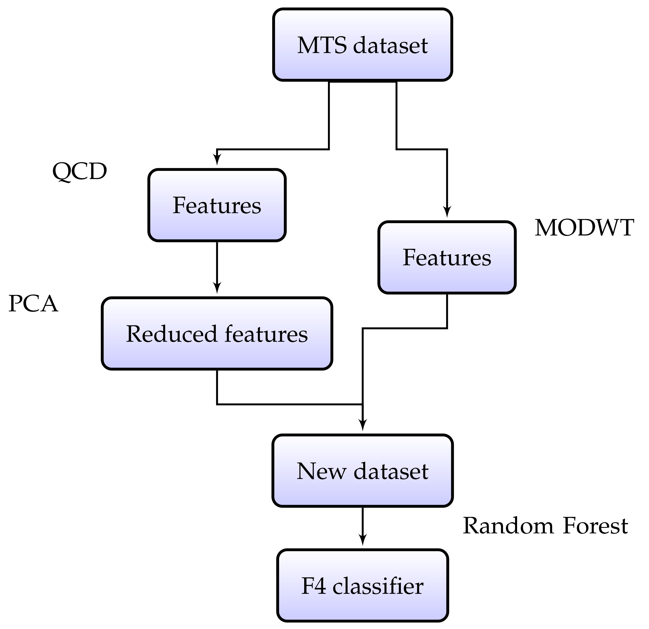
Figure 1 shows a flowchart of F4 classifier.

2.4. Effectiveness of Combining Both Feature Types: An Illustrative Example

Consider a supervised classification problem consisting of three classes, each one of them defined by a linear, nonlinear and conditional heteroskedastic bivariate process, which are given below.

• Class 1

  $$\left(\begin{array}{c}{X}_{t,1}\\ X_{t,2}\end{array}\right)=\left(\begin{array}{cc}0.6& 0.4\\ -0.4& 0.5\end{array}\right)\left(\begin{array}{c}{X}_{t-1,1}\\ X_{t-1,2}\end{array}\right)+\left(\begin{array}{c}{ϵ}_{t,1}\\ {ϵ}_{t,2}\end{array}\right).$$
• Class 2

  $$\begin{array}{c}\hfill \left(\begin{array}{c}{X}_{t,1}\\ X_{t,2}\end{array}\right)=\left(\begin{array}{c}0.9X_{t-1,2}{I}_{\left\{\right|X_{t-1,1}|\le 1\}}-3X_{t-1,1}{I}_{\left\{\right|X_{t-1,1}|>1\}}\\ 0.9X_{t-1,1}{I}_{\left\{\right|X_{t-1,2}|\le 1\}}-3X_{t-1,2}{I}_{\left\{\right|X_{t-1,2}|>1\}}\end{array}\right)+\left(\begin{array}{c}{ϵ}_{t,1}\\ {ϵ}_{t,2}\end{array}\right).\end{array}$$
• Class 3. Let ${(X_{t,1},X_{t,2})}^{⊺}={(a_{t,1},a_{t,2})}^{⊺}={({\sigma }_{t,1}{ϵ}_{t,1},{\sigma }_{t,2}{ϵ}_{t,2})}^{⊺}$, denoting ⊺ the transpose operator. The data-generating process consists of two Gaussian GARCH models

  $${\sigma }_{t,1}^2=0.01+0.05a_{t-1,1}^2+0.94{\sigma }_{t-1,1}^2,$$

  $${\sigma }_{t,2}^2=0.5+0.2a_{t-1,2}^2+0.5{\sigma }_{t-1,2}^2.$$

In the three cases, the vector ${({ϵ}_{t,1},{ϵ}_{t,2})}^{⊺}$ is an i.i.d. vector error process following a bivariate normal distribution with zero mean. The variance of ${ϵ}_{t,1}$ and ${ϵ}_{t,2}$ is 1. The covariance between ${ϵ}_{t,1}$ and ${ϵ}_{t,2}$ is 0 in Classes 1 and 2 and 0.5 in Class 3.

We simulated 50 realisations of length $T=10$ from each class, which were randomly divided into equal sized training and testing sets to assess the performance of classifier F4. The classification was also carried out considering each kind of features separately. The average accuracies based on 400 trials of the simulation mechanism are given in

Table 1. Average accuracy of F4 and the individual classifiers.

Features for Classification	QCD	MODWT	F4
Accuracy	0.651	0.649	0.718

.

Even though the series length is substantially small, the classifiers based only on a feature type (QCD or MODWT) performed significantly better than a naive classifier (which here has an expected accuracy of 0.33). However, the combined classifier F4 led to a higher average score than the individual approaches. With the aim of rigorously confirming the superiority of F4, we performed Wilcoxon–Mann–Whitney tests. The 400 accuracy values obtained by F4 were compared either with the values attained by the QCD-based classifier or the MODWT-based classifier. In both cases, the alternative hypothesis stated that F4 achieves higher accuracy than the single classifier with a probability greater than 0.5. Both p-values were less than $2.2\times {10}^{-16}$, thus indicating rejection of the null hypothesis.

Table 2. Average confusion matrices for the individual (QCD and MODWT) and combined (F4) classifiers.

		QCD			MODWT			F4
		Predicted			Predicted			Predicted
		Class 1	Class 2	Class 3	Class 1	Class 2	Class 3	Class 1	Class 2	Class 3
Actual	Class 1	16.73	3.51	3.76	14.28	5.02	4.70	16.97	3.47	3.56
	Class 2	3.92	15.89	4.19	5.75	15.63	2.62	3.98	17.36	2.66
	Class 3	5.82	5.01	16.18	5.03	3.20	18.77	4.38	3.08	19.54

shows the average confusion matrices based on the 400 trials for QCD, MODWT and F4, respectively. Therefore, the quantities at each matrix add up to 75, the size of the test set. The diagonal elements are related to correct classifications, whereas the off-diagonal elements correspond to the different types of errors. All diagonal elements in the matrix obtained with F4 are greater than the corresponding ones in the other two matrices, thus indicating that F4 performed better than the individual classifiers with regards to the three classes. The greatest improvement occurred in Class 2, associated with the nonlinear MTS. An interesting aspect is that both individual classifiers are prone to different kinds of errors. For example, the QCD-based classifier is more likely to predict Class 3 from a series coming from Class 2, or to predict Class 2 for a series pertaining to Class 3. On the other hand, the MODWT-based classifier is more likely to anticipate Class 1 for an MTS coming from Class 2, or to predict Class 3 for an MTS belonging to Class 1.

It can be deduced from the previous remarks that, in this example, both single classifiers are able to extract from the data complementary information. Thus, the joint use of features extracted via QCD and via MODWT seems a reasonable choice in order to obtain improved performance in an MTSC problem.

3. Experimental Evaluation under Stationary Processes

In this section, we carry out a set of simulations with the aim of assessing the performance of F4 in different scenarios of MTSC. All the generating processes here are stationary. The simulation mechanism and the assessment procedure are properly detailed and the obtained results are presented and discussed.

3.1. Experimental Design

Three supervised classification setups were considered in order to cover a wide variety of stationary generating processes. Specifically, we consider the classification of (1) VARMA (vector autoregressive moving average) processes, (2) nonlinear processes and (3) dynamic conditional correlation processes. This selection is aimed at achieving a fair and general assessment, including indeed pivotal scenarios in many application domains. The specific generating models are given below.

Scenario 1.

VARMA processes classification.

(a)

VAR(1)

$$\left(\begin{array}{c}{X}_{t,1}\\ X_{t,2}\\ X_{t,3}\end{array}\right)=\left(\begin{array}{ccc}0.6& 0.5& 0\\ -0.4& 0.5& 0.3\\ 0& -0.5& 0.7\end{array}\right)\left(\begin{array}{c}{X}_{t-1,1}\\ X_{t-1,2}\\ X_{t-1,3}\end{array}\right)+\left(\begin{array}{c}{ϵ}_{t,1}\\ {ϵ}_{t,2}\\ {ϵ}_{t,3}\end{array}\right),$$

(b)

VAR(1)

$$\left(\begin{array}{c}{X}_{t,1}\\ X_{t,2}\\ X_{t,3}\end{array}\right)=\left(\begin{array}{ccc}0.2& 0.2& 0.1\\ -0.2& 0.2& 0.6\\ 0.1& -0.3& 0.2\end{array}\right)\left(\begin{array}{c}{X}_{t-1,1}\\ X_{t-1,2}\\ X_{t-1,3}\end{array}\right)+\left(\begin{array}{c}{ϵ}_{t,1}\\ {ϵ}_{t,2}\\ {ϵ}_{t,3}\end{array}\right),$$

(c)

VMA(1)

$$\left(\begin{array}{c}{X}_{t,1}\\ X_{t,2}\\ X_{t,3}\end{array}\right)=\left(\begin{array}{ccc}0.6& 0.5& 0\\ -0.4& 0.5& 0.3\\ 0& -0.5& 0.7\end{array}\right)\left(\begin{array}{c}{ϵ}_{t-1,1}\\ {ϵ}_{t-1,2}\\ {ϵ}_{t-1,3}\end{array}\right)+\left(\begin{array}{c}{ϵ}_{t,1}\\ {ϵ}_{t,2}\\ {ϵ}_{t,3}\end{array}\right),$$

(d)

VMA(1)

$$\left(\begin{array}{c}{X}_{t,1}\\ X_{t,2}\\ X_{t,3}\end{array}\right)=\left(\begin{array}{ccc}0.3& 0.1& 0.3\\ -0.2& 0.1& 0.4\\ 0.1& -0.5& 0.4\end{array}\right)\left(\begin{array}{c}{ϵ}_{t-1,1}\\ {ϵ}_{t-1,2}\\ {ϵ}_{t-1,3}\end{array}\right)+\left(\begin{array}{c}{ϵ}_{t,1}\\ {ϵ}_{t,2}\\ {ϵ}_{t,3}\end{array}\right),$$

(e)

VARMA(1,1)

$$\begin{array}{ccc}\hfill \left(\begin{array}{c}{X}_{t,1}\\ X_{t,2}\\ X_{t,3}\end{array}\right)& =& \left(\begin{array}{ccc}0.6& 0.5& 0\\ -0.4& 0.5& 0.3\\ 0& -0.5& 0.7\end{array}\right)\left(\begin{array}{c}{X}_{t-1,1}\\ X_{t-1,2}\\ X_{t-1,3}\end{array}\right)+\hfill \\ & & \left(\begin{array}{ccc}0.6& 0.5& 0\\ -0.4& 0.5& 0.3\\ 0& -0.5& 0.7\end{array}\right)\left(\begin{array}{c}{ϵ}_{t-1,1}\\ {ϵ}_{t-1,2}\\ {ϵ}_{t-1,3}\end{array}\right)+\left(\begin{array}{c}{ϵ}_{t,1}\\ {ϵ}_{t,2}\\ {ϵ}_{t,3}\end{array}\right).\hfill \end{array}$$

In all of the cases, ${({ϵ}_{t,1},{ϵ}_{t,2},{ϵ}_{t,3})}^{⊺}$ is an i.i.d. vector error process following the trivariate normal distribution with zero mean and covariance matrix equals the identity matrix.

Scenario 2.

Nonlinear processes classification.

(a)

NAR (nonlinear autoregressive process)

$$\left(\begin{array}{c}{X}_{t,1}\\ X_{t,2}\end{array}\right)=\left(\begin{array}{c}0.7|X_{t-1,1}|/(|X_{t-1,2}|+1)\\ 0.7|X_{t-1,2}|/(|X_{t-1,1}|+1)\end{array}\right)+\left(\begin{array}{c}{ϵ}_{t,1}\\ {ϵ}_{t,2}\end{array}\right),$$

(b)

TAR (threshold autoregressive process)

$$\left(\begin{array}{c}{X}_{t,1}\\ X_{t,2}\end{array}\right)=\left(\begin{array}{c}0.9X_{t-1,2}{I}_{\left\{\right|X_{t-1,1}|\le 1\}}-0.3X_{t-1,1}{I}_{\left\{\right|X_{t-1,1}|>1\}}\\ 0.9X_{t-1,1}{I}_{\left\{\right|X_{t-1,2}|\le 1\}}-0.3X_{t-1,2}{I}_{\left\{\right|X_{t-1,2}|>1\}}\end{array}\right)+\left(\begin{array}{c}{ϵ}_{t,1}\\ {ϵ}_{t,2}\end{array}\right),$$

(c)

(BL (bilinear process)

$$\left(\begin{array}{c}{X}_{t,1}\\ X_{t,2}\end{array}\right)=\left(\begin{array}{c}0.7X_{t-1,1}{ϵ}_{t-2,2}\\ 0.7X_{t-1,2}{ϵ}_{t-2,1}\end{array}\right)+\left(\begin{array}{c}{ϵ}_{t,1}\\ {ϵ}_{t,2}\end{array}\right),$$

(d)

EXPAR (exponential autoregressive process)

$$\left(\begin{array}{c}{X}_{t,1}\\ X_{t,2}\end{array}\right)=\left(\begin{array}{c}0.3-10exp\left(-X_{t-1,1}^2-X_{t-1,2}^2\right)X_{t-1,2}\\ 0.3-10exp\left(-X_{t-1,1}^2-X_{t-1,2}^2\right)X_{t-1,1}\end{array}\right)+\left(\begin{array}{c}{ϵ}_{t,1}\\ {ϵ}_{t,2}\end{array}\right).$$

In all of the cases, ${({ϵ}_{t,1},{ϵ}_{t,2})}^{⊺}$ is an i.i.d. vector error process following the bivariate normal distribution with zero mean and covariance matrix equals the identity matrix.

Scenario 3.

Dynamic conditional correlation processes classification. Consider ${(X_{t,1},X_{t,2})}^{⊺}={(a_{t,1},a_{t,2})}^{⊺}={({\sigma }_{t,1}{ϵ}_{t,1},{\sigma }_{t,2}{ϵ}_{t,2})}^{⊺}$. The data generating process consists of two GARCH models. Specifically,

$${\sigma }_{t,1}^2=0.01+c_1{a}_{t-1,1}^2+c_2{\sigma }_{t-1,1}^2,$$

$${\sigma }_{t,2}^2=0.5+c_3{a}_{t-1,2}^2+c_4{\sigma }_{t-1,2}^2,$$

$$\left(\begin{array}{c}{ϵ}_{t,1}\\ {ϵ}_{t,2}\end{array}\right)\sim N\left[\left(\begin{array}{c}0\\ 0\end{array}\right),\left(\begin{array}{cc}1& {\rho }_t\\ {\rho }_t& 1\end{array}\right)\right].$$

The coefficients in the GARCH models and the correlation between the standardised shocks, ${\rho }_t$, are given by the following expressions:

(a)

Piecewise constant correlation

$${\rho }_t=0.9I_{\{t\le (T/2\left)\right\}}-0.7I_{\{t>(T/2\left)\right\}},c_1=0.05,c_2=0.94,c_3=0.2,c_4=0.5,$$

(b)

Constant correlation

$${\rho }_t=0.5,c_1=0.075,c_2=0.93,c_3=0.25,c_4=0.5,$$

(c)

Piecewise constant correlation

$${\rho }_t=0.9I_{\{t\le (T/2\left)\right\}}-0.2I_{\{t>(T/2\left)\right\}},c_1=0.10,c_2=0.92,c_3=0.3,c_4=0.5,$$

(d)

Piecewise varying correlation

$$\begin{array}{c}\hfill {\rho }_t=\frac{0.99}{log(t+100)}{I}_{\left\{t\mathrm{odd}\right\}}-\frac{0.99}{log(t+100)}{I}_{\left\{t\mathrm{even}\right\}},\\ \hfill c_1=0.125,c_2=0.91,c_3=0.35,c_4=0.5.\end{array}$$

Scenario 1 constitutes a slight modification of the first scenario in [31] and focuses on the classification of VARMA models. VARMA models are broadly used in many fields but the determination of the models order is quite complex since fixing orders too small leads to inconsistent estimators, whereas too large orders produce less accurate predictions. Our classifier does not require prior modelling and the goal is to assess its capability to learn the underlying model and its accuracy to classify new unlabelled realisations. In particular, Scenario 1 involves up to five classes of different three-dimensional VARMA structures, thus generating a not simple classification framework. Scenario 2 consists of multivariate extensions of univariate NAR, TAR and BL processes presented in [37] and EXPAR process given in [38]. Nonlinear UTS arise in several application fields [39,40,41]. Although nonlinear MTS have received much less attention, there exist some fields, such as neurophysiology [42] and economics [43], in which nonlinear analysis of MTS has proven to be critical. Thus, a good classifier should be able to discriminate between different nonlinear generating processes. Scenario 3 is based on Scenario 2 in [31], which is in turn motivated by a simulation study in the landmark work [44], where dynamic conditional correlation models are introduced. In [31], the GARCH coefficients remained constant between the different classes, being the distinctive features the correlations between the error terms. However, this time, in order to cover a broader picture, each class is characterised by both the correlation between the error terms and the GARCH coefficients. Multivariate GARCH models have been extensively investigated over the last decades (an extensive survey is offered in [45]). Specifically, the estimation of dynamic conditional correlation models has been widely applied to financial series of different nature [46,47,48]. Furthermore, we have decided to include in Scenario 3 both positive and negative correlations, since it has been shown that some financial quantities are either positively or negatively correlated depending on the period [49].

The simulation procedure was carried out as follows. For each process, 50 time series of length $T=50$ (Scenario 1), $T=40$ (Scenario 2) and $T=250$ (Scenario 3) were generated. The whole set of MTS was randomly split into training and test sets, each one of them containing half of the observations. The simulation mechanism was repeated 100 times.

3.2. Alternative Approaches and Assessment Criteria

To shed light on the performance of F4, it was compared with some classical approaches for MTSC. They are summarised below.

• DTW-based classifiers (DTW). The two multivariate extensions of the dynamic time warping distance described in [10] are usually considered as a benchmark in MTS classification (see, e.g., [14,15,16,18]). The “independent” warping version (DTWI) computes DTW between each pair of UTS, whereas the “dependent” version (DTWD) forces all of the dimensions to warp identically, in a single warping matrix. Classification is generally carried out with a nearest neighbour classifier based on these distances. Since both distances produced very similar results, only the outcomes with DTWD are reported, which gave rise to slightly greater average scores.
• Nonparametric approach in the frequency domain (KST). The work of [3] proposed to describe each MTS ${\mathbf{X}}_t$ by means of a set of spectral matrices ${\mathbf{S}}_X$, and then measuring the dissimilarity between a pair of series in terms of the so-called J-divergence, $d_J$, a measure of disparity between the corresponding sets of spectral matrices. In a supervised classification setup with K classes, sets of average spectral density matrices ${\mathbf{S}}_1,\dots ,{\mathbf{S}}_K$ are obtained for each class by considering the training set, and a test observation ${\mathbf{Y}}_t$ is assigned to the class $k^{*}={arg\; min}_{1\le k\le K}{d}_J({\mathbf{S}}_k,{\mathbf{S}}_Y)$. In [31], $d_J$ was tested in cluster analysis, achieving outstanding results when grouping linear processes. Hence, this classifier provides a good benchmark in our Scenario 1.
• Two-dimensional singular value decomposition (2dSVD). The work of [7] introduced 2dSVD, which is an extension of the standard SVD. Two-dimensional singular value decomposition explicitly captures the 2D nature of 2D objects, such as 2D images. MTS row–row and column–column covariance matrices are directly constructed for each MTS and the eigenvectors are computed. The first r and s eigenvectors are retained and each MTS is replaced by the matrix obtained via 2dSVD, which is a function of r and s. Finally, a nearest neighbour classifier considering the Euclidean distances between columns of the resulting matrices is executed. In [6], a comparison between some MTS classifiers is carried out by using three real MTS datasets. The authors considered 2dSVD along with four other approaches [4,5,6], being the results obtained by 2dSVD very close to the best ones. All of the methods are based on dimensionality reduction and SVD. Thus, we have considered that choosing only one of these approaches (2dSVD) is enough to reach satisfactory conclusions about the performance of this type of method in the designed scenarios. The 2dSVD classifier requires the selection of r and s. Our numerical experiments have shown that, in most cases, the higher the number of retained eigenvectors, the better the performance of the classifier. Thus, we have decided to retain all of the eigenvectors from both covariance matrices.
• A versatile approach based on features of different nature (ZK). The work of [24] proposed a generic method to perform MTSC over an arbitrary set of MTS data. Each MTS is described by means of a set of features derived from each UTS (mean, maximal value, skewness, kurtosis, etc.). The cross-correlations between each pair of UTS are also included. The resulting features are then used to feed a random forest. This method produced the second-highest score of nearly 80 participant teams who took part in the 2015 AAIA Data Mining Competition concerned with classifying firefighter activities. Note that this method relies on statistical features as the sample moments, thus being suitable for MTSC based on generating processes.

The random forest algorithm was implemented throughout the paper by means of the function ranger() of the R package ranger, with the default options. Specifically, we considered 500 trees, unlimited depth for each tree and a splitting criterion based on the Gini Index. Concerning the number of variables to possibly split at in each node of the trees, the value $\lfloor \sqrt{P}\rfloor$ was taken into account, P being the number of predictors. Several combinations of hyperparameters were tested in the different scenarios, but usually no improvements were obtained over the default settings. It is worth remarking that this result is in accordance with the fact that the random forest algorithm does not require hyperparameter tuning in most cases [50].

The KST classifier does not need hyperparameter tuning, while DTW and 2dSVD only require to set the number k of neighbours. We considered $k=1$ in both cases since this is the most common choice in the literature. In fact, DTW is usually applied along with the 1NN classifier [1,14,20] and the comparative study carried out in [6] also considered 2dSVD with the 1NN classifier.

The behaviour of the different classifiers was assessed by means of four common performance measures computed with regards to the test set, namely accuracy (ACC), precision (PR), recall (RE) and F1-score (F1). To compute PR and RE, we considered the so-called macro average, which gives the same weight to every class regardless of the number of instances involved. All of the considered metrics take values between 0 and 1 in such a way that the closer to 1 the measure, the better the predictive ability of the classifier.

3.3. Results and Discussion

The averages and standard deviations of the performance measures over the 100 trials are given in

Table 3. Averages and standard deviations (in brackets) of the performance metrics for the five classifiers in Scenarios 1, 2 and 3. For each scenario and metric, the best average result is shown in bold.

	Metric	F4	KST	ZK	2dSVD	DTW
Scenario 1	Accuracy	0.933	0.954	0.806	0.291	0.324
		(0.024)	(0.020)	(0.041)	(0.050)	(0.048)
	Precision	0.937	0.958	0.813	0.528	0.564
		(0.022)	(0.018)	(0.037)	(0.083)	(0.089)
	Recall	0.936	0.954	0.811	0.296	0.327
		(0.022)	(0.020)	(0.039)	(0.042)	(0.041)
	F1-score	0.934	0.954	0.806	0.210	0.244
		(0.023)	(0.020)	(0.040)	(0.106)	(0.113)
Scenario 2	Accuracy	0.882	0.854	0.805	0.403	0.380
		(0.041)	(0.036)	(0.044)	(0.049)	(0.056)
	Precision	0.886	0.862	0.808	0.610	0.647
		(0.040)	(0.038)	(0.043)	(0.059)	(0.050)
	Recall	0.886	0.855	0.808	0.404	0.382
		(0.036)	(0.035)	(0.042)	(0.042)	(0.045)
	F1-score	0.878	0.845	0.799	0.321	0.300
		(0.042)	(0.038)	(0.047)	(0.074)	(0.077)
Scenario 3	Accuracy	0.952	0.635	0.867	0.329	0.600
		(0.025)	(0.058)	(0.032)	(0.041)	(0.064)
	Precision	0.953	0.675	0.869	0.376	0.648
		(0.024)	(0.050)	(0.032)	(0.047)	(0.069)
	Recall	0.953	0.633	0.869	0.328	0.601
		(0.024)	(0.056)	(0.031)	(0.026)	(0.060)
	F1-score	0.951	0.616	0.865	0.080	0.577
		(0.025)	(0.064)	(0.033)	(0.125)	(0.070)

. According to these results, F4 was the best performing classifier in Scenarios 2 and 3, and the runner-up in Scenario 1. In this latter scenario, the KST classifier achieved the best results, only slightly above those obtained by F4. Zagorecki’s approach achieved acceptable results, but quite far from those of the top performers. The remaining competitors, DTW and 2dSVD, attained very poor scores, only slightly improving the expected accuracy of a naive classifier (0.20).

As for Scenario 2, F4 and KST continued to be the approaches receiving the highest scores, the former slightly outperforming the latter. Here, ZK obtained results close to the top classifiers. Finally, KST significantly worsened its performance in Scenario 3, where only F4 (with scores close to one for all of the metrics) and ZK obtained satisfactory results. Classifier DTW obtained its highest average scores in this scenario.

Table 3 allows us to conclude that F4 was, on average, the most effective classifier in the considered settings. The combined use of QCD- and MODWT-based features gives F4 enough versatility to achieve excellent scores when facing either linear, nonlinear or conditionally heteroskedastic processes.

To gain more insights into the previous remarks, the top panels in Figure 2, Figure 3 and Figure 4 display the boxplots based on the performance measures of the 100 simulation trials for Scenarios 1, 2 and 3, respectively. The graphs clearly show that the weak spot of KST is Scenario 3, where its performance substantially worsened. F4 and ZK showed a more stable behaviour, maintaining similar scores along the three considered scenarios. DTW and 2dSVD always received, on average, higher scores for PR than for RE. Therefore, these classifiers did a worse job finding the observations of a given class than getting the right decision over the test observations assigned to a particular class. Interestingly enough, the dynamic time warping-based approach obtained acceptable results in Scenario 3, receiving an average accuracy of 0.6.

The average accuracy over all of the 300 trials for F4, the QCD- and the MODWT-based classifiers was $0.922$, $0.861$ and $0.849$, respectively. Therefore, as in the motivating example of Section 2.4, F4 produced significantly greater scores than its solo counterparts, thus illustrating the importance of considering simultaneously both types of features.

We also checked the behaviour of the classifiers under some amount of fat-tailedness in the error distribution. Note that this characteristic is frequently exhibited by either UTS and MTS arising in several application domains [51,52,53,54], which motivated us to analyse its effect in our experiments. The whole simulation was replicated with errors generated from a multivariate t distribution with 3 degrees of freedom and the results are given in

Table 4. Averages and standard deviations (in brackets) of the performance metrics for the five classifiers in Scenarios 1, 2 and 3 with heavy tails. For each scenario and metric, the best average result is shown in bold.

	Metric	F4	KST	ZK	2dSVD	DTW
Scenario 1	Accuracy	0.918	0.734	0.714	0.296	0.315
		(0.029)	(0.087)	(0.046)	(0.043)	(0.065)
	Precision	0.921	0.773	0.722	0.469	0.588
		(0.028)	(0.069)	(0.045)	(0.079)	(0.085)
	Recall	0.921	0.736	0.720	0.300	0.320
		(0.028)	(0.087)	(0.042)	(0.039)	(0.057)
	F1-score	0.918	0.720	0.709	0.232	0.220
		(0.029)	(0.100)	(0.046)	(0.106)	(0.121)
Scenario 2	Accuracy	0.832	0.647	0.753	0.403	0.390
		(0.045)	(0.063)	(0.053)	(0.049)	(0.070)
	Precision	0.840	0.722	0.763	0.610	0.672
		(0.040)	(0.057)	(0.05)	(0.059)	(0.099)
	Recall	0.837	0.643	0.758	0.404	0.387
		(0.041)	(0.065)	(0.049)	(0.042)	(0.057)
	F1-score	0.830	0.625	0.751	0.321	0.273
		(0.045)	(0.075)	(0.053)	(0.074)	(0.116)
Scenario 3	Accuracy	0.903	0.442	0.804	0.577	0.589
		(0.034)	(0.075)	(0.042)	(0.051)	(0.055)
	Precision	0.906	0.521	0.809	0.576	0.589
		(0.033)	(0.070)	(0.038)	(0.053)	(0.060)
	Recall	0.906	0.439	0.807	0.578	0.592
		(0.034)	(0.070)	(0.040)	(0.048)	(0.054)
	F1-score	0.902	0.390	0.802	0.561	0.576
		(0.035)	(0.086)	(0.04)	(0.053)	(0.057)

.

In this new situation, F4 achieved the best average scores in the three considered scenarios, followed by KST in Scenario 1 and by ZK in Scenarios 2 and 3. Whereas F4 and ZK slightly decreased their average effectiveness when heavy tails were introduced, KST suffered a substantial decline for all of the performance metrics. The distance-based approaches, 2dSVD and DTW, obtained poor results in Scenarios 1 and 2, and higher scores in Scenario 3. Surprisingly, 2dSVD improved its behaviour under heavy tails in Scenario 3. The corresponding boxplots are depicted in the bottom panels of Figure 2, Figure 3 and Figure 4. All of the plots clearly show that F4 outperformed the remaining competitors by a large margin. Whereas Zagorecki’s approach ZK showed again a stable behaviour, the decline suffered by KST due to the distributional form of the errors was so substantial that it was beaten by 2dSVD and DTW in Scenario 3 regardless of the considered performance measure.

4. Experimental Evaluation under Nonstationary Processes

In this section, the simulation study is extended to examine the performance of F4 when coping with some types of nonstationary processes.

4.1. Experimental Design

Two new classification scenarios involving exploding VAR (vector autoregressive) processes and VAR processes with time-varying coefficients (tVAR) were considered. The specific generating models concerning each class of processes are given below.

Scenario 4.

Explosive VAR processes classification.

(a)

VAR(1)

$$\left(\begin{array}{c}{X}_{t,1}\\ X_{t,2}\\ X_{t,3}\end{array}\right)=\left(\begin{array}{ccc}1.01& 0.9& 0\\ -0.8& 0.9& 0.8\\ 0& -0.9& 0.9\end{array}\right)\left(\begin{array}{c}{X}_{t-1,1}\\ X_{t-1,2}\\ X_{t-1,3}\end{array}\right)+\left(\begin{array}{c}{ϵ}_{t,1}\\ {ϵ}_{t,2}\\ {ϵ}_{t,3}\end{array}\right),$$

(b)

VAR(1)

$$\left(\begin{array}{c}{X}_{t,1}\\ X_{t,2}\\ X_{t,3}\end{array}\right)=\left(\begin{array}{ccc}1.03& 0.95& 0\\ -0.85& 0.6& 0.8\\ 0& -0.95& 0.9\end{array}\right)\left(\begin{array}{c}{X}_{t-1,1}\\ X_{t-1,2}\\ X_{t-1,3}\end{array}\right)+\left(\begin{array}{c}{ϵ}_{t,1}\\ {ϵ}_{t,2}\\ {ϵ}_{t,3}\end{array}\right).$$

Scenario 5.

Time-varying VAR processes classification.

(a)

tVAR(1)

$$\left(\begin{array}{c}{X}_{t,1}\\ X_{t,2}\end{array}\right)=\left(\begin{array}{cc}0.49cos(t\pi /2T)& 0.49cos(t\pi /2T)\\ 0.49cos(t\pi /2T)& 0.49\end{array}\right)\left(\begin{array}{c}{X}_{t-1,1}\\ X_{t-1,2}\end{array}\right)+\left(\begin{array}{c}{ϵ}_{t,1}\\ {ϵ}_{t,2}\end{array}\right),$$

(b)

tVAR(1)

$$\left(\begin{array}{c}{X}_{t,1}\\ X_{t,2}\end{array}\right)=\left(\begin{array}{cc}0.01cos(t\pi /2T)& 0.01cos(t\pi /2T)\\ 0.01cos(t\pi /2T)& -0.3\end{array}\right)\left(\begin{array}{c}{X}_{t-1,1}\\ X_{t-1,2}\end{array}\right)+\left(\begin{array}{c}{ϵ}_{t,1}\\ {ϵ}_{t,2}\end{array}\right).$$

In all of the cases, the error is an i.i.d. process following a multivariate standard Gaussian distribution. The generating models in Scenario 4 correspond to nonstationary processes since their coefficient matrices have eigenvalues with a modulus greater than one (see, e.g., Chapter 2 in [55]). These kinds of VAR processes are usually referred to as explosive. Explosive VAR processes have been shown to naturally arise in some disciplines, such as macroeconomics [56]. The matrices of coefficients in Scenario 5 vary with t, thus making the processes nonstationary despite verifying the stationarity conditions for each t. This scenario is a multivariate extension of the scenario of Simulation 2 in [57]. Time-varying VAR models have empirical applications in monetary policy [58] or in estimating fiscal and monetary interactions, among others [59]. Thus, Scenarios 4 and 5 are two examples of nonstationary processes commonly encountered in practice.

It is worth pointing out that the classifier F4 is based on quantile cross-spectral densities, which are not defined for nonstationary processes. However, the sample quantities ${\widehat{G}}_{T,R}^{j_1,j_2}(\omega ,\tau ,{\tau }^{\prime })$ always exist and can be computed as descriptive features, even if they do not have a direct interpretation in a nonstationary setting. Since the target is not modelling the underlying processes but properly learning an algorithm to classify unlabelled MTS accurately, the relevant issue is whether or not the sample features provide distinct spectral characterisations of different nonstationarity structures. To illustrate the usefulness of QCD in Scenario 4, we have depicted in Figure 5 estimates of the quantile cospectrum and quantile quadrature spectrum between $X_{t,1}$ and $X_{t,3}$ for large sample size simulations ($T=2000$) of the two models involved in this scenario. The probability levels ${\tau }_1=0.1$ and ${\tau }_2=0.5$ were considered. The left panels refer to particular realisations of the processes, whereas the right panels refer to different ones. Each line has been plotted with a distinct intensity level of red and blue according to the underlying class. It can be deduced from the plots that both estimates tend to the same quantities within a given class as the series length approaches infinity, and these limits are different between the two classes. Similar situations occur when a different pair of variables and quantile levels are taken into account. Thus, it is expected that F4 can appropriately discriminate between both classes in Scenario 4. Analogous conclusions can be obtained for Scenario 5.

4.2. Results and Discussion

The simulation procedure was carried out along the same lines as for the stationary scenarios in Section 3.1 except for the series lengths, which were $T=60$ in Scenario 4 and $T=100$ in Scenario 5. The averages and standard deviations of the performance metrics are provided in

Table 5. Averages and standard deviations (in brackets) of the performance metrics for the five classifiers in Scenarios 4 and 5. For each scenario and metric, the best average result is shown in bold.

	Metric	F4	KST	ZK	2dSVD	DTW
Scenario 4	Accuracy	1	1	0.952	0.902	0.894
		(0)	(0)	(0.033)	(0.054)	(0.049)
	Precision	1	1	0.955	0.905	0.903
		(0)	(0)	(0.031)	(0.053)	(0.042)
	Recall	1	1	0.953	0.903	0.895
		(0)	(0)	(0.033)	(0.052)	(0.048)
	F1-score	1	1	0.952	0.901	0.892
		(0)	(0)	(0.033)	(0.054)	(0.050)
Scenario 5	Accuracy	1	1	0.980	0.776	0.788
		(0)	(0)	(0.024)	(0.072)	(0.079)
	Precision	1	1	0.980	0.814	0.853
		(0)	(0)	(0.023)	(0.060)	(0.853)
	Recall	1	1	0.980	0.780	0.791
		(0)	(0)	(0.025)	(0.068)	(0.791)
	F1-score	1	1	0.979	0.769	0.775
		(0)	(0)	(0.025)	(0.076)	(0.775)

. The classifiers KST and F4 achieved perfect results in both scenarios, followed by ZK, which performed pretty well, especially in Scenario 5. The classifiers 2dSVD and DTW received worse scores, Scenario 5 being particularly challenging for these methods.

5. Effect of the Size of the Training Set and the Series Length

This section is devoted to analysing how the effectiveness of the five considered classifiers behaves according to the series length T and the amount of training data M. To do so, 100 simulation trials of Scenario 2 were performed for different values of T and M, namely $T\in \{10,20,40,60,80,100\}$ and $M\in \{40,80,200,400,600,800\}$. When varying the value of T, the value of M remained constant, $M=200$, whereas when varying the value of M, the value of T remained constant, $T=40$. Note that these values of M and T were the ones utilised in the simulations of Scenario 2 in Section 3.

The curves of average accuracies as a function of T and M are shown in the top and bottom panels of Figure 6, respectively. F4, ZK and KST increased their accuracy with the series length, which was expected because these classifiers are feature-based and the true features are more accurately estimated with larger realisations. For values of T beyond 60, the rate of increase was greater for F4 than for ZK and KST. As for 2dSVD and DTW, they obtained worse results as T got larger, eventually approaching the accuracy associated with a naive classifier (0.20). This seems counterintuitive at first, but it has a logical explanation. These approaches are based on separating geometric profiles, and when the series length is small, they are able to discriminate between classes to some degree. However, as the series get longer, the classification task depends more and more on removing the noise, which is complex for these classifiers, and they are no longer able to distinguish between generating processes. With regards to the effect of adding more training data, classifiers F4, ZK and 2dSVD seem to benefit from this fact, the increase in accuracy being considerably slight for $M>400$. On the other hand, the effectiveness of KST and DTW does not seem to significantly vary across the different values of M. It is worth mentioning that F4 and ZK are the only approaches benefiting from both an increase of the series length and the amount of training data.

6. Time Consumption Comparison

To assess the computational efficiency of the five classifiers analysed throughout the paper, we have recorded the runtime spent by the corresponding programs in finishing the classification task regarding Scenario 2. Note that, for some approaches, as F4 and ZK, the classification process consists of feature extraction followed by the construction of a random forest. In contrast, for other approaches, such as DTW, the classification procedure consists directly of the computation of a distance between each element in the test set and all of the elements in the training set. We consider that the classification task is over when all of the performance measures regarding the test set have been computed. We recorded the running times for $(M,T)\in \left\{\right(200,40),(200,80),(400,40\left)\right\}$, with M and T denoting the amount of training data and the MTS length, respectively. With the aim of mitigating the uncertainty caused by uncontrollable factors, we have taken the running time over the 100 simulation trials. The computer used to run the programs was a MacBook Pro with processor Quad-Core Intel Core i7, a speed of 2.9 GHz and a RAM memory of 16 GB. The programs were coded and executed in RStudio. The R version was 3.6.1.

The CPU runtime for the five methods is given in

Table 6. The CPU runtime (minutes) for the five classifiers regarding the 100 simulation trials in Scenario 2. Different values for the amount of training data (M) and the length of the series (T) were considered.

Classifier	$\mathit{M}=\mathbf{200}$, $\mathit{T}=\mathbf{40}$	$\mathit{M}=\mathbf{200}$, $\mathit{T}=\mathbf{80}$	$\mathit{M}=\mathbf{400}$, $\mathit{T}=\mathbf{40}$
F4	4.239	5.125	7.017
KST	86.524	102.177	197.480
ZK	3.510	3.573	4.927
2dSVD	26.279	26.304	67.686
DTW	37.154	186.986	80.018

. The most efficient classifier was ZK, closely followed by F4, while the less efficient ones were KST and DTW. The classifier 2dSVD lies somewhere in the middle. The linear increase in time suffered by the distance-based classifier DTW when adding more training data was expected due to the approach employed by these classifier. Unlike the rest of the methods, DTW was affected to a large extent when the series length increased. With regards to F4 and ZK, their running times grew less than linearly with M and T. In summary, besides getting the best average results in our experiments, F4 has shown to be one of the most efficient classifiers.

7. Application to ECG Data

In this section, F4 is applied to a common MTSC problem: discriminating between ECG signals coming from subjects suffering from myocardial infarction (MI) and ECG signals from healthy subjects. This problem has been extensively studied in the medical literature [26,60,61,62]. It is worth remarking that ECG signals are known to be nonstationary.

The considered data come from the PTB Diagnostic ECG Database [63]. Specifically, we have downloaded the database from the Kaggle repository (https://www.kaggle.com/openmark/ptb-diagnostic-ecg-database (accessed on 2 October 2021)), containing 448 15-lead ECG signals from 148 MI patients (368 instances) and 52 healthy volunteers (80 instances). The minimum series length in this MTS dataset is T = 32,000. This database has been broadly used for ECG classification [26,64,65,66,67]. Before performing the classification task, we have decided to make the following preprocessing steps.

• The first 80 ECG records from MI patients and all of the records from healthy controls were considered to have a balanced classification problem. This way, the results are more easily interpretable, as a naive classifier is expected to achieve an accuracy of 0.5 in the new dataset.
• For the sake of simplicity and reasonable computation times, the first 6 leads and 500 time observations of each ECG signal were selected. The choice of certain subsets of dimensions and time observations is common in ECG classification [26,62].

In summary, the considered dataset consists of 160 6-lead ECG signals of length $T=500$, 80 pertaining to MI patients and 80 coming from healthy controls. Figure 7 displays a signal of each class. The top panel shows the ECG of a subject suffering from MI, whereas the bottom panel displays a signal of a healthy volunteer.

F4 and the competitors regarded throughout this work were used to perform the classification task. As this dataset does not contain a training–testing default split, we took the following steps in order to properly evaluate the classifiers.

• Randomly splitting the original dataset into training and testing datasets, each one of them containing 80 ECG signals.
• Fitting each classifier in the training set and evaluating its effectiveness in the test set.

Hyperparameter selection for classifiers F4 and ZK was made in the same way as in the simulations. Methods 2dSVD and DTW were used again along with the 1NN classifier. Steps 1 and 2 before were repeated 10 times and the average accuracies are given in

Table 7. Average accuracies of the five classifiers in the ECG database. The best result is shown in bold.

Classifier	F4	ZK	KST	2dSVD	DTW
Accuracy	0.860	0.800	0.693	0.554	0.568

. F4 obtained the best average score, 0.860, and ZK also performed pretty well. On the contrary, the approaches 2dSVD and DTW achieved poor results. They were virtually unable to discriminate between the two classes of ECG signals. The classifier KST lay in the middle. These results illustrate the usefulness of the F4 classifier in an important and active field of research as it is ECG classification.

8. Application to Some UEA Datasets

We now apply F4 to some datasets in the UEA multivariate time series classification archive. Training and testing sets are given in the archive for each dataset, thus allowing to perform a rigorous assessment of new MTSC algorithms. Notice that our goal here is not running F4 in each and every dataset and comparing the results with those that are state of the art. This would be unfair for F4, as it does not contain any shape or level-based information, such as the mean or the maximal or minimal values of each UTS constituting the given MTS, which are known to be proper discriminative features for the datasets in the archive (a simple graphical analysis of some MTS confirms this fact). Instead, we want to show how F4, which is mainly aimed at discriminating between generating processes, can also obtain good results when dealing with some real-life classification problems in which each class is characterised by a different geometric profile.

The considered datasets are summarised in

Table 8. Summary of the six datasets from the UEA multivariate time series classification archive.

Dataset	Train Cases	Test Cases	Dimensions	Length	Classes
Cricket	108	72	6	1197	12
Libras	180	180	2	45	15
Epilepsy	137	138	3	206	4
RacketSports	151	152	6	30	4
Handwriting	150	850	3	152	26
BasicMotions	40	40	6	100	4

. They cover a broad variety of dimensions, series lengths and numbers of classes, thus constituting a heterogeneous subset of the UEA archive. Each dataset in Table 8 pertains to a different problem. For instance, the data in RacketSports were created from university students playing badminton or squash while wearing a smart watch, the problem being to identify the sport and the stroke of each player. A summary of the corresponding problems can be seen in [20].

The F4 algorithm, along with its competitors, was used to perform MTSC in the six considered datasets. We maintained the same setting considered throughout the work. Accuracies obtained in the test set are given in

Table 9. Accuracies of the five classifiers in the six datasets from the UEA multivariate time series classification archive.

Dataset	F4	KST	ZK	2dSVD	DTW
Cricket	1	0.986	0.986	0.931	1
Libras	0.861	0.422	0.894	0.811	0.872
Epilepsy	1	0.877	0.978	0.587	0.884
RacketSports	0.888	0.447	0.849	0.816	0.816
Handwriting	0.433	0.179	0.280	0.328	0.621
BasicMotions	1	1	1	0.600	0.750
Average	0.864	0.652	0.831	0.679	0.824

. F4 got the best average results in these challenging scenarios, showing its huge versatility. It clearly beat KST and 2dSVD, and reaped better results than ZK and DTW in four out of the six datasets.

As a matter of fact, F4 attained perfect results with the datasets containing series of large length (Cricket, Epilepsy and Basic Motions), and worse results with the datasets containing series of short length (Libras and RacketSports). The exception to this fact was the dataset Handwriting. F4 achieved the worst results in this dataset. However, this could be due to the large number of existing classes (26), which makes the classification task in Handwriting particularly challenging. The previous insights are not surprising, since a larger value of the series length implies a more accurate estimate of QCD and the wavelet quantities. This suggests that F4 could be particularly useful when dealing with datasets containing long MTS.

9. Conclusions and Future Work

Given the massive amount of data that are generated everyday, TSC has become a topic of paramount importance. MTSC is a more challenging task than UTSC given the high dimensionality of MTS objects. Classification of MTS should take into account the relationships between dimensions. Whereas most of the approaches for MTSC are based on considering that the different classes are described by means of unequal geometric profiles, only a few authors have tackled the classification task from a point of view of multivariate generating processes. The first contribution of this paper was addressing that issue by proposing F4, a versatile, effective and efficient classifier for MTSC. F4 consists of two steps: feature extraction via QCD and MODWT, and feeding a traditional random forest classifier with the extracted features. F4 was tested in a wide variety of simulated scenarios, including stationary and nonstationary settings. In all of the considered cases, F4 led to very good results, comparing favourably with some powerful classifiers proposed in the literature.

The great performance of F4 when dealing with nonstationary MTS called for its evaluation in some real datasets, which are usually comprised of nonstationary series. Particularly, the UEA multivariate time series classification archive provided a good starting point. Actually, we were sceptical about F4 performing well in these datasets. Furthermore, we did not suspect that F4 would be able to beat ZK and DTW in some of them. The classes in these datasets are often characterised by changes in level and other shape patterns, and neither of them are taken into consideration by F4, which is mainly based on the dependence structure within and between MTS dimensions. Thus, another contribution of this work was to show that even in an MTSC problem calling for a shape-based classifier, a dependence-based classifier could be helpful.

Finally, F4 was also used to solve a classical problem in medicine: classifying ECG signals of MI and healthy patients. The approach was successful in discriminating between both types of signals in a well-known ECG dataset.

There are two main ways through which this work could be further developed. First, an extension of F4 considering the inclusion of geometric features could be constructed. This way, classification performance is likely to improve substantially, at least when coping with datasets such as the ones in the UEA archive. Indeed, we have already obtained promising preliminary results by considering this approach. Second, it would be interesting to design an even computationally cheaper version of F4 to properly cope with situations in which the number of dimensions becomes considerably large. Both approaches will be properly addressed in upcoming months.

References

1. Wu, J.; Yao, L.; Liu, B. An overview on feature-based classification algorithms for multivariate time series. In Proceedings of the 2018 3rd IEEE International Conference on Cloud Computing and Big Data Analysis, ICCCBDA 2018, Chengdu, China, 20–22 April 2018; pp. 32–38. [Google Scholar]
2. Handhika, T.; Murni; Lestari, D.P.; Sari, I. Multivariate time series classification analysis: State-of-the-art and future challenges. In IOP Conference Series: Materials Science and Engineering, Proceedings of the International Conference on Science and Innovated Engineering (I-COSINE), Aceh, Indonesia, 21–22 October 2018; IOP Publishing: Bristol, UK, 2019; Volume 536, p. 012003. [Google Scholar]
3. Kakizawa, Y.; Shumway, R.H.; Taniguchi, M. Discrimination and clustering for multivariate time series. J. Am. Stat. Assoc. 1998, 93, 328–340. [Google Scholar] [CrossRef]
4. Li, C.; Khan, L.; Prabhakaran, B. Real-time classification of variable length multi-attribute motions. Knowl. Inf. Syst. 2006, 10, 163–183. [Google Scholar] [CrossRef]
5. Li, C.; Khan, L.; Prabhakaran, B. Feature selection for classification of variable length multiattribute motions. In Multimedia Data Mining and Knowledge Discovery; Springer: Berlin/Heidelberg, Germany, 2007; pp. 116–137. [Google Scholar]
6. Weng, X.; Shen, J. Classification of multivariate time series using locality preserving projections. Knowl.-Based Syst. 2008, 21, 581–587. [Google Scholar] [CrossRef]
7. Ding, C.; Ye, J. 2-dimensional singular value decomposition for 2D maps and images. In Proceedings of the 2005 SIAM International Conference on Data Mining, SDM 2005, Neport Beach, CA, USA, 21–23 April 2005; Society for Industrial and Applied Mathematics: Philadelphia, PA, USA, 2005; pp. 32–43. [Google Scholar]
8. Jeong, Y.S.; Jeong, M.K.; Omitaomu, O.A. Weighted dynamic time warping for time series classification. Pattern Recognit. 2011, 44, 2231–2240. [Google Scholar] [CrossRef]
9. Kate, R.J. Using dynamic time warping distances as features for improved time series classification. Data Min. Knowl. Discov. 2016, 30, 283–312. [Google Scholar] [CrossRef]
10. Shokoohi-Yekta, M.; Hu, B.; Jin, H.; Wang, J.; Keogh, E. Generalizing DTW to the multi-dimensional case requires an adaptive approach. Data Min. Knowl. Discov. 2017, 31, 1–31. [Google Scholar] [CrossRef] [Green Version]
11. Mei, J.; Liu, M.; Wang, Y.F.; Gao, H. Learning a mahalanobis distance-based dynamic time warping measure for multivariate time series classification. IEEE Trans. Cybern. 2015, 46, 1363–1374. [Google Scholar] [CrossRef]
12. Bankó, Z.; Abonyi, J. Correlation based dynamic time warping of multivariate time series. Expert Syst. Appl. 2012, 39, 12814–12823. [Google Scholar] [CrossRef]
13. Górecki, T.; Łuczak, M. Multivariate time series classification with parametric derivative dynamic time warping. Expert Syst. Appl. 2015, 42, 2305–2312. [Google Scholar] [CrossRef]
14. Ruiz, A.P.; Flynn, M.; Bagnall, A. Benchmarking Multivariate Time Series Classification Algorithms. arXiv 2020, arXiv:2007.13156. [Google Scholar]
15. Karim, F.; Majumdar, S.; Darabi, H.; Harford, S. Multivariate LSTM-FCNs for time series classification. Neural Netw. 2019, 116, 237–245. [Google Scholar] [CrossRef] [Green Version]
16. Schäfer, P.; Leser, U. Multivariate time series classification with WEASEL+ MUSE. arXiv 2017, arXiv:1711.11343. [Google Scholar]
17. Schäfer, P.; Leser, U. Fast and accurate time series classification with weasel. In Proceedings of the 2017 ACM on Conference on Information and Knowledge Management, Singapore, 6–10 November 2017; pp. 637–646. [Google Scholar]
18. Baydogan, M.G.; Runger, G. Learning a symbolic representation for multivariate time series classification. Data Min. Knowl. Discov. 2014, 29, 400–422. [Google Scholar] [CrossRef]
19. Lines, J.; Taylor, S.; Bagnall, A. Time series classification with HIVE-COTE: The hierarchical vote collective of transformation-based ensembles. ACM Trans. Knowl. Discov. Data 2018, 12. [Google Scholar] [CrossRef] [Green Version]
20. Bagnall, A.; Dau, H.A.; Lines, J.; Flynn, M.; Large, J.; Bostrom, A.; Southam, P.; Keogh, E. The UEA multivariate time series classification archive, 2018. arXiv 2018, arXiv:1811.00075. [Google Scholar]
21. Karim, F.; Majumdar, S.; Darabi, H.; Chen, S. LSTM Fully Convolutional Networks for Time Series Classification. IEEE Access 2017, 6, 1662–1669. [Google Scholar] [CrossRef]
22. Liu, C.L.; Hsaio, W.H.; Tu, Y.C. Time series classification with multivariate convolutional neural network. IEEE Trans. Ind. Electron. 2018, 66, 4788–4797. [Google Scholar] [CrossRef]
23. Fang, H.; Shrestha, A.; Qiu, Q. Multivariate time series classification using spiking neural networks. In Proceedings of the 2020 International Joint Conference on Neural Networks (IJCNN), Glasgow, UK, 19–24 July 2020; pp. 1–7. [Google Scholar]
24. Zagorecki, A. A versatile approach to classification of multivariate time series data. In Proceedings of the 2015 Federated Conference on Computer Science and Information Systems, FedCSIS 2015, Lodz, Poland, 13–16 September 2015; Volume 5, pp. 407–410. [Google Scholar]
25. Meina, M.; Janusz, A.; Rykaczewski, K.; Slkezak, D.; Celmer, B.; Krasuski, A. Tagging Firefighter Activities at the Emergency Scene: Summary of AAIA’15 Data Mining Competition at Knowledge Pit. Ann. Comput. Sci. Inf. Syst. 2015, 5, 367–373. [Google Scholar]
26. Maharaj, E.A.; Alonso, A.M. Discriminant analysis of multivariate time series: Application to diagnosis based on ECG signals. Comput. Stat. Data Anal. 2014, 70, 67–87. [Google Scholar] [CrossRef]
27. Formisano, E.; De Martino, F.; Valente, G. Multivariate analysis of fMRI time series: Classification and regression of brain responses using machine learning. Magn. Reson. Imaging 2008, 26, 921–934. [Google Scholar] [CrossRef] [PubMed]
28. Seto, S.; Zhang, W.; Zhou, Y. Multivariate time series classification using dynamic time warping template selection for human activity recognition. In Proceedings of the 2015 IEEE Symposium Series on Computational Intelligence, Cape Town, South Africa, 7–10 December 2015; pp. 1399–1406. [Google Scholar]
29. Hassan, S.A.; Malik, F. Multivariate GARCH modeling of sector volatility transmission. Q. Rev. Econ. Financ. 2007, 47, 470–480. [Google Scholar] [CrossRef]
30. Anderson, C.W.; Stolz, E.A.; Shamsunder, S. Multivariate autoregressive models for classification of spontaneous electroencephalographic signals during mental tasks. IEEE Trans. Biomed. Eng. 1998, 45, 277–286. [Google Scholar] [CrossRef] [PubMed]
31. López-Oriona, Á.; Vilar, J.A. Quantile cross-spectral density: A novel and effective tool for clustering multivariate time series. Expert Syst. Appl. 2021, 185, 115677. [Google Scholar] [CrossRef]
32. Durso, P.; Maharaj, E.A. Wavelets-based clustering of multivariate time series. Fuzzy Sets Syst. 2012, 193, 33–61. [Google Scholar] [CrossRef]
33. Baruník, J.; Kley, T. Quantile coherency: A general measure for dependence between cyclical economic variables. Econom. J. 2019, 22, 131–152. [Google Scholar] [CrossRef] [Green Version]
34. Coppi, R.; D’Urso, P. The geometric approach to the comparison of multivariate time trajectories. In Advances in Classification and Data Analysis; Springer: Berlin/Heidelberg, Germany, 2001; pp. 93–100. [Google Scholar]
35. Breiman, L. Random forests. Mach. Learn. 2001, 45, 5–32. [Google Scholar] [CrossRef] [Green Version]
36. Friedman, J.H. Greedy function approximation: A gradient boosting machine. Ann. Stat. 2001, 29, 1189–1232. [Google Scholar] [CrossRef]
37. Zhang, G.P.; Patuwo, B.E.; Hu, M.Y. A simulation study of artificial neural networks for nonlinear time-series forecasting. Comput. Oper. Res. 2001, 28, 381–396. [Google Scholar] [CrossRef]
38. Lafuente-Rego, B.; Vilar, J.A. Clustering of time series using quantile autocovariances. Adv. Data Anal. Classif. 2016, 10, 391–415. [Google Scholar] [CrossRef]
39. Granger, C.W.J.; Terasvirta, T. Modelling non-linear economic relationships. In OUP Catalogue; Oxford University Press: Oxford, UK, 1993. [Google Scholar]
40. Granger, C.W.J.; Andersen, A.P. An Introduction to Bilinear Time Series Models; Vandenhoeck und Rupreckt: Gottingen, Germany, 1978. [Google Scholar]
41. Tong, H.; Lim, K.S. Threshold autoregression, limit cycles and cyclical data. In Exploration Of A Nonlinear World: An Appreciation of Howell Tong’s Contributions to Statistics; World Scientific: Singapore, 2009; pp. 9–56. [Google Scholar]
42. Pereda, E.; Quiroga, R.Q.; Bhattacharya, J. Nonlinear multivariate analysis of neurophysiological signals. Prog. Neurobiol. 2005, 77, 1–37. [Google Scholar] [CrossRef] [Green Version]
43. Koop, G.; Pesaran, M.H.; Potter, S.M. Impulse response analysis in nonlinear multivariate models. J. Econom. 1996, 74, 119–147. [Google Scholar] [CrossRef]
44. Engle, R. Dynamic conditional correlation: A simple class of multivariate generalized autoregressive conditional heteroskedasticity models. J. Bus. Econ. Stat. 2002, 20, 339–350. [Google Scholar] [CrossRef]
45. Bauwens, L.; Laurent, S.; Rombouts, J.V. Multivariate GARCH models: A survey. J. Appl. Econom. 2006, 21, 79–109. [Google Scholar] [CrossRef] [Green Version]
46. Ku, Y.H.H.; Chen, H.C.; Chen, K.H. On the application of the dynamic conditional correlation model in estimating optimal time-varying hedge ratios. Appl. Econ. Lett. 2007, 14, 503–509. [Google Scholar] [CrossRef]
47. Naoui, K.; Liouane, N.; Brahim, S. A dynamic conditional correlation analysis of financial contagion: The case of the subprime credit crisis. Int. J. Econ. Financ. 2010, 2, 85–96. [Google Scholar] [CrossRef] [Green Version]
48. Kuper, G.H. Dynamic conditional correlation analysis of financial market interdependence: An application to Thailand and Indonesia. J. Asian Econ. 2007, 18, 670–684. [Google Scholar] [CrossRef] [Green Version]
49. Andersson, M.; Krylova, E.; Vähämaa, S. Why does the correlation between stock and bond returns vary over time? Appl. Financ. Econ. 2008, 18, 139–151. [Google Scholar] [CrossRef]
50. Probst, P.; Wright, M.N.; Boulesteix, A.L. Hyperparameters and tuning strategies for random forest. Wiley Interdiscip. Rev. Data Min. Knowl. Discov. 2019, 9, e1301. [Google Scholar] [CrossRef] [Green Version]
51. Harvey, A.C. Dynamic Models for Volatility and Heavy Tails: With Applications to Financial and Economic Time Series; Cambridge University Press: Cambridge, UK, 2013; Volume 52. [Google Scholar]
52. Anderson, P.L.; Meerschaert, M.M. Modeling river flows with heavy tails. Water Resour. Res. 1998, 34, 2271–2280. [Google Scholar] [CrossRef] [Green Version]
53. Weron, R. Heavy-tails and regime-switching in electricity prices. Math. Methods Oper. Res. 2009, 69, 457–473. [Google Scholar] [CrossRef] [Green Version]
54. Davis, R.A.; Heiny, J.; Mikosch, T.; Xie, X. Extreme value analysis for the sample autocovariance matrices of heavy-tailed multivariate time series. Extremes 2016, 19, 517–547. [Google Scholar] [CrossRef] [Green Version]
55. Reinsel, G.C. Elements of Multivariate Time Series Analysis; Springer Science & Business Media: New York, NY, USA, 2003. [Google Scholar]
56. Qureshi, H. Explosive Roots in Level Vector Autoregressive Models. Technical Report. 2008. Available online: https://core.ac.uk/download/pdf/7199482.pdf (accessed on 3 October 2021).
57. Alonso, A.M.; Casado, D.; López-Pintado, S.; Romo, J. Robust functional supervised classification for time series. J. Classif. 2014, 31, 325–350. [Google Scholar] [CrossRef]
58. Primiceri, G.E. Time varying structural vector autoregressions and monetary policy. Rev. Econ. Stud. 2005, 72, 821–852. [Google Scholar] [CrossRef]
59. Gerba, E.; Hauzenberger, K. Estimating US Fiscal and Monetary Interactions in a Time Varying VAR; Technical Report, School of Economics Discussion Papers; University of Kent: Canterbury, UK, 2013. [Google Scholar]
60. Diker, A.; Cömert, Z.; Avcı, E. A diagnostic model for identification of myocardial infarction from electrocardiography signals. Bitlis Eren Univ. J. Sci. Technol. 2017, 7, 132–139. [Google Scholar] [CrossRef]
61. Liu, B.; Liu, J.; Wang, G.; Huang, K.; Li, F.; Zheng, Y.; Luo, Y.; Zhou, F. A novel electrocardiogram parameterization algorithm and its application in myocardial infarction detection. Comput. Biol. Med. 2015, 61, 178–184. [Google Scholar] [CrossRef] [PubMed]
62. Sadhukhan, D.; Pal, S.; Mitra, M. Automated identification of myocardial infarction using harmonic phase distribution pattern of ECG data. IEEE Trans. Instrum. Meas. 2018, 67, 2303–2313. [Google Scholar] [CrossRef]
63. Goldberger, A.L.; Amaral, L.A.; Glass, L.; Hausdorff, J.M.; Ivanov, P.C.; Mark, R.G.; Mietus, J.E.; Moody, G.B.; Peng, C.K.; Stanley, H.E. PhysioBank, PhysioToolkit, and PhysioNet: Components of a new research resource for complex physiologic signals. Circulation 2000, 101, e215–e220. [Google Scholar] [CrossRef] [Green Version]
64. Kachuee, M.; Fazeli, S.; Sarrafzadeh, M. Ecg heartbeat classification: A deep transferable representation. In Proceedings of the 2018 IEEE International Conference on Healthcare Informatics (ICHI), New York, NY, USA, 4–7 June 2018; pp. 443–444. [Google Scholar]
65. Remya, R.; Indiradevi, K.; Babu, K.A. Classification of myocardial infarction using multi resolution wavelet analysis of ECG. Procedia Technol. 2016, 24, 949–956. [Google Scholar] [CrossRef] [Green Version]
66. Banerjee, S.; Mitra, M. ECG feature extraction and classification of anteroseptal myocardial infarction and normal subjects using discrete wavelet transform. In Proceedings of the 2010 International Conference on Systems in Medicine and Biology, Kharagpur, India, 16–18 December 2010; pp. 55–60. [Google Scholar]
67. Banerjee, S.; Mitra, M. Application of cross wavelet transform for ECG pattern analysis and classification. IEEE Trans. Instrum. Meas. 2013, 63, 326–333. [Google Scholar] [CrossRef]
Figure 1. Flowchart of F4 classifier.
Mathematics 09 03051 g001
Figure 2. Boxplots of accuracy, precision, recall and F1-score based on the 100 trials of the simulation procedure for Scenario 1 (top panel) and for Scenario 1 with heavy tails (bottom panel).
Mathematics 09 03051 g002
Figure 3. Boxplots of accuracy, precision, recall and F1-score based on 100 trials of the simulation procedure for Scenario 2 (top panel) and for Scenario 2 with heavy tails (bottom panel).
Mathematics 09 03051 g003
Figure 4. Boxplots of accuracy, precision, recall and F1-score based on 100 trials of the simulation procedure for Scenario 3 (top panel) and for Scenario 3 with heavy tails (bottom panel).
Mathematics 09 03051 g004
Figure 5. Estimates of the hypothetical quantile cospectrum and quantile quadrature spectrum between X t , 1 and X t , 3 for large sample size ( T = 2000 ) simulations of processes (a) and (b) in Scenario 4. The left hand panels correspond to particular realisations of both processes, whereas the right hand panels to other realisations.
Mathematics 09 03051 g005
Figure 6. Average accuracies of the five classifiers as a function of the series length (top panel) and the amount of training data (bottom panel). One hundred simulation trials of Scenario 2 were considered for each value of T and M.
Mathematics 09 03051 g006
Figure 7. ECG of a patient suffering from MI (top panel) and of a healthy volunteer (bottom panel).
Mathematics 09 03051 g007