An Extended Reweighted ${\ell }_1$ Minimization Algorithm for Image Restoration

Abstract

This paper proposes an effective extended reweighted ${\ell }_1$ minimization algorithm (ERMA) to solve the basis pursuit problem $\underset{u\in R^n}{\min }\{{||u||}_1:Au=f\}$ in compressed sensing, where $A\in R^{m\times n}$, $m\ll n$. The fast algorithm is based on linearized Bregman iteration with soft thresholding operator and generalized inverse iteration. At the same time, it also combines the iterative reweighted strategy that is used to solve $\underset{u\in R^n}{\min }\{{||u||}_p^p:Au=f\}$ problem, with the weight ${\omega }_i(u,p)={(\epsilon +{|u_i|}^2)}^{p/2-1}$. Numerical experiments show that this ${\ell }_1$ minimization persistently performs better than other methods. Especially when $p=0$, the restored signal by the algorithm has the highest signal to noise ratio. Additionally, this approach has no effect on workload or calculation time when matrix A is ill-conditioned.

1. Introduction

Image restoration is a fundamental problem in image processing. In particular, image deblurring has great application for facial alignment, remote sensing, medical image processing, camera equipment, compression transmission, and so on [1,2,3].

Let $u\in R^n$ be an original signal with $k$ nonzero components ($u$ is called $k$—sparse signal or vector) and $f\in R^m$ be the linear measurements with the form $Au=f$ for some $A\in R^{m\times n}$,$m\ll n$. Then, the compressed sensing problem can be represented as (1), where ${||u||}_0$ is the number of nonzero elements of vector $u$.

The main purpose of compressive sensing is to recover the sparse signal from the inaccurate linear measurements. Namely, we shall identify valid algorithms for efficiently solving the indeterminate linear system.

Unfortunately, the ${\ell }_0$ minimization problem (1) is nonconvex and generally cannot be solved fast and efficiently. A common alternative is to consider the convex-relaxation of (1), i.e., basis pursuit problem [4,5]. The solution of the linear equations $Au=f$ may not exist, and measurement $f$ may contain noise in certain applications. Thus, under such occasions we need to compute its least square solution.

There has been a recent flurry of study in compressive sensing, which entails resolving problems (2). Candes et al. [6,7], Donoho [8,9], and others were the driving force behind this, as detailed in [6,7,8,10,11,12,13,14,15,16,17,18]. The theory of compressed sensing assures that solving (2) under specific restrictions on the dense matrix $A$ and the sparsity of $u$ will yield the sparsest solution of $Au=f$. However, there are no universal linear programming strategies for handling this problem. As a result, [6] presents a soft threshold linearized Bregman iteration, and [9,14,19,20,21] investigates its associated convergence. Unfortunately, only $A$ is surjective. Cai et al. then studied linearized Bregman iteration with soft threshold where $A$ is any matrix and its property in [19,22]. In [23], Qiao et.al proposed a simplified iterative formula that combines original linearized Bregman iteration together with iterative formula for generalized inverse of matrix $A\in R^{m\times n}$,$m\ll n$, and soft threshold. In [24,25], Liu et al. proposed efficient non-convex total variation ${\ell }_1-{\ell }_2$ with differential shrink operator.

$$\underset{u\in R^n}{\min }{||u||}_0 s.t. Au=f$$

(1)

$$\underset{u\in R^n}{\min }\{{||u||}_1:Au=f\}.$$

(2)

On the basis of this, Qiao et.al proposed Chaotic Iteration for compressed sensing and image deblurring in [26,27]. Chaotic Iteration not only possesses all merits of linearized Bregman iterative method, but also accelerates the computing speed. Subsequently, we were inspired by the reweighted idea in [27,28,29] and proposed the reweighted ℓ₁ minimization algorithm with $\omega$-inverse function (RMA-IF) based on Chaotic Iteration in [27]. We are interested in the fact that the restored effect of RMA-IF is better than Chaotic Iteration without increasing the computing time. Unfortunately, in [27], we only discussed the case that the weight coefficient is a usual inverse function. It did not involve the general weight coefficients and any theoretical results of the corresponding algorithms. This is exactly what this paper does.

In addition, it was also shown in [23] that exact reconstruction can be achieved by a nonconvex variant of basis pursuit with fewer measurements. Precisely, the ${\ell }_1$ norm is replaced by the ${\ell }_p$ quasi-norm.

$$\underset{u\in R^n}{\min }\{{||u||}_p^p:Au=f\}$$

(3)

where ${||u||}_p={({\displaystyle \sum }_i{|u_i|}^p)}^{\raisebox{1ex}{$1$}\!\left/ \!\raisebox{-1ex}{$p$}\right.}$, $0\le p\le 1$.

However, the ${\ell }_p$ quasi-norm is nonconvex for $0<p<1$, and ${\ell }_p$ minimization is generally NP-hard problem. Instead of directly minimizing the ${\ell }_p$ quasi-norm, which most likely ends up with one of its numerous local minimizers, these algorithms [30,31] solve a series of smoothed subproblems. Specifically, [32] solves reweighted ${\ell }_1$ subproblems: given an existing iterate $u^k$, the algorithm generates a new iterate $u^{(k+1)}$ by minimizing ${\displaystyle \sum }_i{\omega }_i|u_i|$ with weights ${\omega }_i={(|u_i|+\epsilon )}^{p-1}$. In [33], Xiu et al. illustrated the reweighted algorithm in order to solve the variational model ${\ell }_1-{\ell }_p$. On the other hand, the works in [34,35,36] solve reweighted ${\ell }_2$ subproblems: at each iteration, they approximate ${||u||}_p^p$ by ${\displaystyle \sum }_i{\omega }_i{|u_i|}^2$ with weights ${\omega }_i={({|u_i|}^2+\epsilon )}^{\frac{p}{2}-1}$. To recover a sparse vector u from $Au=f$, these algorithms need to vary $\epsilon$, starting at a large value and gradually reducing it. Empirical results show that the sparsity of the signal can be enhanced by the reweighted coefficients in the algorithm, so that the algorithm can recover the signal quickly. The reweighted ${\ell }_1$ or ${\ell }_2$ algorithms require much less measurements than convex ${\ell }_1$ minimization to recover vectors with entries in decaying magnitudes, and in compressed sensing, this measurement reduction corresponds to savings in sensing time and cost.

In this paper, we propose a reweighted ${\ell }_1$ minimization algorithm for the basis pursuit problem (2) in compressed sensing. The algorithm is based on Chaotic Iteration [23] and iterative reweighted strategy that is used to solve the $\underset{u\in R^n}{\min }\{{||u||}_p^p:Au=f\}$ problem. In particular, we chose the weight coefficient that given in papers [31,32,34,35,36,37] and let parameter $p=0$,1$,\frac{1}{2},\frac{2}{3}$ in numerical experiment [38].

The rest of the paper is organized as follows. The available strategies for tackling the confined problem (2) are summarized in Section 2. The reweighted ${\ell }_1$ minimization algorithm is described, and convergence behavior is also analyzed in Section 3. In Section 4, the numerical results are shown. Finally, in Section 5, we draw some conclusions.

2. Preliminaries

2.1. $A^{+}$ Linearized Bregman Iteration

In [22], Cai et al. extended linearized Bregman iteration to

$$\{\begin{array}{l}{f}^{(k+1)}=f^k+f-A{u}^k\\ u^{(k+1)}=\delta T_u(A^{+}{f}^{(k+1)})\end{array}$$

(4)

where $f$ is a known measurement, and $Au=f,$ $f^{(0)}=0, u^{(0)}=0$; $A^{+}$ is Moore–Penrose generalized inverse matrix of any $A$, and

$$T_{\mu }(\omega )≔{\left[t_{\mu }({\omega }_1),t_{\mu }({\omega }_2)\dots t_{\mu }({\omega }_n)\right]}^T$$

(5)

is the soft thresholding operator [6] with

$$t_{\mu }(\xi )=\{\begin{array}{l}0, |\xi |\le \mu , \\ sgn(\xi )(|\xi |-\mu ), |\xi |>\mu .\end{array}$$

(6)

Theorem 1. 

[39] Let $A\in R^{m\times n}$, $m\ll n$, be an arbitrary matrix. Then, the sequence${\{u^{(k)}\}}_{k\in N}$generated by (4) with $0<\delta <1$converges to the unique solution of

$$\underset{u\in R^n}{\min }\{\mu {||u||}_1+\frac{1}{2\delta }{||u||}_2^2:u=\arg \underset{u\in R^n}{\min }||Au={f||}_2^2\}$$

(7)

Furthermore, when $\mu \to \infty$, the limit of ${\{u^{(k)}\}}_{k\in N}$tends to the solution of

$$\underset{u\in R^n}{\min }\{{||u||}_1:u=\arg \underset{u\in R^n}{\min }||Au={f||}_2^2\}$$

(8)

that has a minimal${\ell }_2$ norm among all the solution of (8).

2.2. Chaotic Iteration

In [20], we noted that the computation of $A^{+}$ involving decomposition of singular value for algorithm (4) needs matrix product, so the computational costs are relatively large. In fact, we just need to compute $A^{+}{f}^{(k+1)}$ in (4). In [26], replacing SVD by iterative computation of $A^{+}$, we obtained Chaotic Iteration. Because the algorithm only needs to calculate the product of matrix and vector, the computing speed is improved without reducing the accuracy.

Chaotic Iteration:

$$\{\begin{array}{l}{f}^{(k+1)}=f^k+f-A{u}^k\\ y^{(k+1)}=y^{(k)}+V_0{f}^{(k+1)}-V_0(A{y}^{(k)}),k=0,1,2,\dots \\ u^{(k+1)}=\delta T_u(y^{(k+1)})\end{array}$$

(9)

where $y_0=V_0{f}^{(0)}$, $V_0=\alpha A^T$, and $0<\alpha <\frac{2}{{||A||}_2^2}$, and $Au=f,$ $f^{(0)}=0$.

Theorem 2. 

[26] Let $A\in R^{m\times n}$, $m\ll n$, be an arbitrary matrix. Assuming the initial value$V_0=\alpha A^{*}, 0<\alpha <\frac{2}{{||A||}_2^2}$, then the sequence${\{u^{(k)}\}}_{k\in N}$generated by (9) with $0<\delta <1$ converges to the unique solution of (7). Furthermore, when $\mu \to \infty$, the limit of ${\{u^{(k)}\}}_{k\in N}$ tends to the solution of (8), which has a minimal ${\ell }_2$ norm among all the solution of (8).

2.3. Reweighted ${\ell }_1$ Minimization Algorithm with $\omega$-Inverse Function Iteration

In order to further improve the chaotic iteration, we combined it with the reweighted strategy in [27]. As a preliminary idea, we chose the usual inverse function as the weight coefficient.

RMA-IF:

$$\{\begin{array}{l}{f}^{(k+1)}=f^k+f-A{u}^k\\ y^{(k+1)}=y^{(k)}+V_0{f}^{(k+1)}-V_0(A{y}^{(k)}),k=0,1,2,\dots \\ u^{(k+1)}=\delta T_{\mu {\omega }^{(k)}}(y^{(k+1)}) ,\\ {\omega }_i^{(k+1)}=1/(|u_i^{(k+1)}|+\epsilon ), i=1,2,\dots ,n\end{array}$$

(10)

where $f^{(0)}=0, y^{(0)}=V_0{f}^{(0)}$, and $Au=f,$ $0<\alpha <\frac{2}{{||A||}_2^2}$, and

$$T_{\mu \omega }(\omega )≔{\left[t_{\mu }({\omega }_1),t_{\mu \omega }({\omega }_2)\dots t_{\mu \omega }({\omega }_n)\right]}^T$$

(11)

is the weighted soft thresholding operator with

$$t_{\mu }(\xi )=\{\begin{array}{l}0, |\xi |\le \mu \omega , \\ sgn(\xi )(|\xi |-\mu ), |\xi |>\mu \omega .\end{array}$$

(12)

3. Reweighted ${\ell }_1$ Minimization Algorithm

Consider the weighted ${\ell }_1$ minimization problem

$$\underset{u\in R^n}{\min }\{{{\displaystyle \sum }}_i{\omega }_i|u_i|:Au=f\}$$

(13)

where $i=1,2,\dots ,n$, are positive weights. Denoting ${\displaystyle \sum }_i{\omega }_i|u_i|$ as ${||u||}_{\omega }$, then (13) can be rewritten as

$$\underset{u\in R^n}{\min }\{{||u||}_{\omega }:Au=f\}$$

(14)

Just like its unweighted counterpart (2), this convex problem can be recast as a linear program. The weighted ${\ell }_1$ minimization (14) can be viewed as relaxation of weighted ${\ell }_0$ minimization problem. Whenever the solution of (1) is unique, it is also the unique solution of weighted ${\ell }_0$ minimization problem, provided that the weights do not vanish. However, the corresponding ${\ell }_1$ relaxations (2) and (14) will have different solutions in general. Hence, one may think of the weights $\omega$ as free parameters in the convex relaxation, whose values if set wisely could improve the signal reconstruction.

In comparison to many algorithms that can be used to solve the problem (2), Chaotic Iteration is very effective [26]. Avoiding computing $A^{+}$ in algorithm (4), the algorithm can reduce the computational complexity and improve the computational efficiency. Thus, we adopt a proper reweight coefficient to this algorithm and obtain a new fast reweighted minimization algorithm.

$$\{\begin{array}{l}{f}^{(k+1)}=f^k+f-A{u}^k\\ y^{(k+1)}=y^{(k)}+V_0{f}^{(k+1)}-V_0(A{y}^{(k)}),k=0,1,2,\dots \\ u^{(k+1)}=\delta T_{\mu {\omega }^{(k)}}(y^{(k+1)}) ,\\ {\omega }_i^{(k+1)}=\omega (u_i^{(k+1)}), i=1,2,\dots ,n\end{array}$$

(15)

where $f^{(0)}=0, u^{(0)}=0, y^{(0)}=V_0{f}^{(0)}$, $V_0=\alpha A^{*}, 0<\alpha <\frac{2}{{||A||}_2^2}$, and $T_{\mu {\omega }^{(k)}}(·)$ is weighted soft thresholding operator, and $\omega (·)$ is weighted function of $u^{(k)}$.

There are many ways to update the weight coefficients $\omega (·)$, and ERMA uses the following schemes:

$$\omega (u^{(k)},p)={(|u^{(k)}|+\epsilon )}^{p-1}$$

(16)

$$\omega (u^{(k)},p)={({|u^{(k)}|}^2+\epsilon )}^{p/2-1}$$

(17)

where $0<p⟨1,\epsilon ⟩0$ avoids division by zero. In [28], weight coefficients (16) and (17) for ${\ell }_p$, $0\le p\le 1$ problem are discussed. We adopt iterative formula (16) and (17), when $p=0$,1$,\frac{1}{2},\frac{2}{3}$. Obviously, these values of $p$ are representative. RMA-IF and Chaotic Iteration are special cases of ERMA with weight coefficients (16), respectively, when $p=0$ and $p=1$.

In [27], we mentioned the weighted soft thresholding operator $T_{\mu \omega }(·)$, and now we expand further discussed about it in the following.

Theorem 3.

$T_{\mu \omega }(\nu =arg\underset{u\in R^n}{\min }\{\mu {||u||}_{\omega }+\frac{1}{2}||u-{\nu ||}_2^2\})$.

Proof. 

Let $f(u)=\mu {||u||}_{\omega }+\frac{1}{2}||u-{\nu ||}_2^2=\mu {\displaystyle \sum }_{i=1}^n{\omega }_i|u_i|+\frac{1}{2}{\displaystyle \sum }_{i=1}^n{({\nu }^{(k)}-u_i)}^2,$ then,

$$\frac{\partial f(u)}{\partial u_i}=\{\begin{array}{l}\mu {\omega }_i+u_i-{\nu }_i^{(k)}, u_i>0 , \\ -\mu {\omega }_i+u_i-{\nu }_i^{(k)}, u_i<0.\end{array}$$

(18)

Case 1: ${\nu }_i^{(k)}>\mu {\omega }_i>0$

(a)

If $u_i>0$, and notice that $\frac{\partial f(u)}{\partial u_i}=0$ then $u_i={\nu }_i^{(k)}-\mu {\omega }_i>0$; for this case, $f(u)$ gets its minimum at point $u_i={\nu }_i^{(k)}-\mu {\omega }_i>0$ along direction $e_i$, and the minimum is:

$$f{(u)|}_{u_i={\nu }_i^{(k)}-\mu {\omega }_i}=\mu {\omega }_i({\nu }_i^{(k)}-\mu {\omega }_i)+\frac{1}{2}{(\mu {\omega }_i)}^2+{\delta }_1(>0)={\mathsf{\Delta }}_1+{\delta }_1$$

(19)

(b)

If $u_i<0$, and notice that $\frac{\partial f(u)}{\partial u_i}=u_i-{\nu }_i^{(k)}-\mu {\omega }_i<0$, again we have that $f(u)$ decreases along direction $e_i$:

$$f{(u)|}_{u_i=0}=\frac{1}{2}{({\nu }_i^{(k)})}^2+{\delta }_1(>0)={\mathsf{\Delta }}_2+{\delta }_1.$$

(20)

Since ${\mathsf{\Delta }}_2+{\mathsf{\Delta }}_1=\frac{1}{2}{({\nu }_i^{(k)})}^2-(\mu {\omega }_i{\nu }_i^{(k)}-\frac{1}{2}{(\mu {\omega }_i)}^2)=\frac{1}{2}{({\nu }_i^{(k)}-\mu {\omega }_i)}^2$, along direction $e_i$, we have the knowledge that the minimizer of $f(u)$ is $u_i={\nu }_i^{(k)}-\mu {\omega }_i$.

Case 2: ${\nu }_i^{(k)}<-\mu {\omega }_i<0$

(a)

If $u_i>0$, since $\frac{\partial f(u)}{\partial u_i}=u_i-{\nu }_i^{(k)}+$ $\mu {\omega }_i>0$, $f(u)$ increases along direction $e_i$.

$$f{(u)|}_{u_i=0}=\frac{1}{2}{({\nu }_i^{(k)})}^2+{\delta }_3(>0)={\mathsf{\Delta }}_3+{\delta }_3$$

(21)

(b)

If $u_i<0$, since $\frac{\partial f(u)}{\partial u_i}=0$, we have $u_i={\nu }_i^{(k)}+\mu {\omega }_i<0$; the minimizer of $f(u)$ along direction $e_i$ is $u_i={\nu }_i^{(k)}+\mu {\omega }_i$, and the corresponding minimum is:

$$f{(u)|}_{u_i={\nu }_i^{(k)}+\mu {\omega }_i}=-\mu {\omega }_i({\nu }_i^{(k)}-\mu {\omega }_i)+\frac{1}{2}{(\mu {\omega }_i)}^2+{\delta }_3(>0)={\mathsf{\Delta }}_4+{\delta }_3$$

(22)

Since ${\mathsf{\Delta }}_3-{\mathsf{\Delta }}_4=\frac{1}{2}{({\nu }_i^{(k)})}^2+(\mu {\omega }_i{\nu }_i^{(k)}+\frac{1}{2}{(\mu {\omega }_i)}^2)=\frac{1}{2}{({\nu }_i^{(k)}+\mu {\omega }_i)}^2>0$, we can obtain the minimizer of $f(u)$ at $u_i={\nu }_i^{(k)}+\mu {\omega }_i$ along direction $e_i$.

Case 3: $-\mu {\omega }_i\le {\nu }_i^{(k)}\le \mu {\omega }_i$

(a)

If $u_i>0$, since $\frac{\partial f(u)}{\partial u_i}=u_i-{\nu }_i^{(k)}+$ $\mu {\omega }_i>0$, $f(u)$ increases along direction $e_i$.

$$f{(u)|}_{u_i=0}=\frac{1}{2}{({\nu }_i^{(k)})}^2+{\delta }_2(>0)$$

(23)

(b)

If $u_i<0$, since $\frac{\partial f(u)}{\partial u_i}=u_i-{\nu }_i^{(k)}-$ $\mu {\omega }_i<0$, $f(u)$ decreases along direction $e_i$.

$$f{(u)|}_{u_i=0}=\frac{1}{2}{({\nu }_i^{(k)})}^2+{\delta }_2$$

(24)

when $u_i=0$, the minimum of $f(u)$ along direction $e_i$ is $f(u)=\frac{1}{2}{({\nu }_i^{(k)})}^2+{\delta }_2$.

In conclusion, we have the weighted soft shrinkage operator (12), and the minimizer of the minimization problem is given by

$$\begin{array}{cc}\hfill u& =arg\underset{u\in R^n}{\min }\{\mu {||u||}_{\omega }+\frac{1}{2}||u-{\nu ||}_2^2\}\hfill \\ & =\{\begin{array}{c}{\nu }_i^{(k)}-\mu {\omega }_i, {\nu }_i^{(k)}>\mu {\omega }_i>0 \\ 0, -\mu {\omega }_i\le {\nu }_i^{(k)}\le \mu {\omega }_i\\ {\nu }_i^{(k)}+\mu {\omega }_i, {\nu }_i^{(k)}<-\mu {\omega }_i<0 \end{array}\hfill \\ & ={\left[t_{\mu }({\omega }_1), t_{\mu }({\omega }_2)\dots t_{\mu }({\omega }_n)\right]}^T\hfill \\ & =T_{\mu \omega }({\nu }^{(k)})\hfill \end{array}$$

(25)

Taking $L_{\mu \omega }(u)=\mu {||u||}_{\omega }+\frac{1}{2}||u-{\nu ||}_2^2$, we provide an analysis of the convergence behavior of ERMA. The main result is the following theorem. □

Theorem 4.

Let$A\in R^{m\times n}$, and$m\ll n$be an arbitrary matrix. Assume the initial value $V_0=\alpha A^{*}, 0<\alpha <\frac{2}{{||A||}_2^2}$, then the sequence ${\{u^{(k)}\}}_{k\in N}$ generated by ERMA ($0\le p\le 1$), then for $0<\delta <\frac{1}{{||A||}_2||A^T||{}_2}$, $\mu >0$ and $\omega >0$.

(a)

$\{L_{\mu \omega }(u^{(k)})\}$ is a monotonically decreasing sequence and bounded below;

(b)

${\{u^{(k)}\}}_{k\in N}$ is asymptotically regular, such that $\underset{k\to \infty }{\lim }||u^{(k+1)}-u^{(k)}||{}_2=0$;

(c)

$L_{\mu \omega }(u^{(k)})$ converges to $L_{\mu \omega }(u^{*})$, where $u^{*}$ is a limit point of function ${\{u^{(k)}\}}_{k\in N}$.

Proof. 

Denote the k-th approximation of objective function $L_{\mu \omega }(u^{(k)})$ as $h(u,u^{(k)})$.

$$h(u,u^{(k)})=\mu {||u||}_{\omega }+\frac{1}{2\delta }||u-{(u^{(k)}-\delta A^T(A{u}^{(k)}-f))||}_2^2$$

(26)

It is easy to see that

$$L_{\mu \omega }(u)=h(u,u^{(k)})+\frac{1}{2}||A{(u-u^{(k)})||}_2^2-\frac{1}{2\delta }||u-u^{(k)}||{}_2^2+C$$

(27)

where $C=-\frac{\delta }{2}||A^T(A{u}^{(k)}-f)||{)}_2^2+\frac{1}{2}||A{u}^{(k)}-f||{)}_2^2$.

(a)

On the basis of the above derivation, we can get

$$\begin{gathered} L_{\mu \omega }(u)=h(u^{(k+1)},u^{(k)})+\frac{1}{2}||A{(u^{(k+1)}-u^{(k)})||}_2^2-\frac{1}{2\delta }||u^{(k+1)}-u^{(k)}||{}_2^2+C \\ \le h(u,u^{(k)})+\frac{1}{2}||A{(u^{(k+1)}-u^{(k)})||}_2^2-\frac{1}{2\delta }||u^{(k+1)}-u^{(k)}||{}_2^2+C \\ =L_{\mu \omega }(u^{(k)})+\frac{1}{2}||A{(u^{(k+1)}-u^{(k)})||}_2^2-\frac{1}{2\delta }||u^{(k+1)}-u^{(k)}||{}_2^2+C<L_{\mu \omega }(u^{(k)}) \end{gathered}$$

(28)

Since $u^{(k+1)}$ is a minimization of $h(u,u^{(k)})$, then the first inequality is satisfied. Again, $0<\delta <\frac{1}{{||A||}_2||A^T||{}_2}$; this implies $\frac{1}{2}||A{(u^{(k+1)}-u^{(k)})||}_2^2-\frac{1}{2\delta }||u^{(k+1)}-u^{(k)}||{}_2^2<0$, the last inequality holds. In additon, for all $k$, $0\le L_{\mu \omega }(u^{(k)})\le L_{\mu \omega }(u^{(0)})=\frac{1}{2}{||f||}_2^2$. Therefore, $\{L_{\mu \omega }(u^{(k)})\}$ is a monotonically decreasing sequence and bounded below.

(b)

From (28), we have

$$L_{\mu \omega }(u^{(k)})-L_{\mu \omega }(u^{(k+1)})\ge \frac{1}{2\delta }||u^{(k+1)}-u^{(k)}||{}_2^2-\delta ||A{(u^{(k+1)}-u^{(k)})||}_2^2$$

(29)

so

$$\begin{gathered} (1-\delta {||A||}_2^2)||u^{(k+1)}-u^{(k)}||{}_2^2\le ||u^{(k+1)}-u^{(k)}||{}_2^2-\delta ||A{(u^{(k+1)}-u^{(k)})||}_2^2 \\ \le 2\delta (L_{\mu \omega }(u^{(k)})-L_{\mu \omega }(u^{(k+1)})) \end{gathered}$$

(30)

thus,

$$||u^{(k+1)}-u^{(k)}||{}_2^2\le \frac{2\delta }{1-\delta {||A||}_2^2}(L_{\mu \omega }(u^{(k)})-L_{\mu \omega }(u^{(k+1)})$$

(31)

Sum of (31) form $0$ to $\mathrm{N}$, we have that

$$\begin{gathered} ||u^{(k+1)}-u^{(k)}||{}_2^2\le \frac{2\delta }{1-\delta {||A||}_2^2}{{\displaystyle \sum }}_{k=0}^N(L_{\mu \omega }(u^{(k)})-L_{\mu \omega }(u^{(k+1)})) \\ \le \frac{2\delta }{1-\delta {||A||}_2^2}{L}_{\mu \omega }(u^{(0)}) \end{gathered}$$

(32)

Therefore, the series ${\displaystyle \sum }_{k=0}^N||u^{(k+1)}-u^{(k)}||{}_2^2$ is convergent and $||u^{(k+1)}-u^{(k)}||{}_2^2\to 0$ as $k\to \infty$.

(c)

Set $u^{(0)}=0$, $\forall k$ from (32), we obtain

$$||u^{(k+1)}||{}_2^2\le {{\displaystyle \sum }}_{j=0}^j||u^{(j+1)}-u^{(j)}||{}_2^2\le \frac{2\delta }{1-\delta {||A||}_2^2}{L}_{\mu \omega }(u^{(0)})$$

(33)

Thus, the sequence $\{u^{(k)}\}$ is bounded and has a convergent subsequence $\{u^{(k_i)}\}\subset \{u^{(k)}\}$. Obviously, $u^{*}=\underset{i\to \infty }{\lim }{u}^{(k_i)}$. To prove $u^{*}=\underset{i\to \infty }{\lim }{u}^{(k)}$, we only need to prove that $\underset{i\to \infty }{\lim }{u}^{(l_i)}=u^{*}$ for any convergent sequence $\{u^{(l_i)}\}\subset \{u^{(k)}\}.$

Let $\underset{i\to \infty }{\lim }{u}^{(l_i)}={\nu }^{*}$ and $u^{*}-{\nu }^{*}=d\ne 0$. That is, there is a constant $K_1>0$ such that, for $\forall l_i>K_1$, we have $|u^{(l_i)}-{\nu }^{*}|<\frac{|d|}{3}$. Moreover, because $\underset{k\to \infty }{\lim }{u}^{\mathrm{k}}={\nu }^{*}$, there $\exists K_2>0$ such that, for $\forall l_i>K_2$ we have $|u^{(k_i)}-u^{*}|<\frac{|d|}{3}$. Therefore,

$$\begin{gathered} |u^{(l_i)}-u^{(k_i)}|=|u^{(l_i)}-{\nu }^{*}+u^{*}-u^{(k_i)}+{\nu }^{*}-u^{*}| \\ \ge |{\nu }^{*}-u^{*}|-|u^{(l_i)}-{\nu }^{*}|-|u^{*}-u^{(k_i)}|\ge \frac{|d|}{3} \end{gathered}$$

(34)

This is contradictory to the regularity in (b). Therefore, $L_{\mu \omega }(u^{(k)})$ converges to a fixed value $L_{\mu \omega }(u^{*})$, where $\underset{k\to \infty }{\lim }{u}^{\mathrm{k}}=u^{*}$. □

4. Numerical Result

In the basis pursuit problem (2), the constraint $Au=f$ is underdetermined linear equations. We test ERMA with (16) (${\omega }_1$) and (17) (${\omega }_2$) when $p=0$,1$,\frac{1}{2},\frac{2}{3}$ for the problem (2), respectively. Here, the quality of restoration is measured by the signal-to-noise ratio (SNR), structural similarity (SSIM), and mean squared error (MSE) defined by

$$SNR(u)≔20{\log }_{10}\left(\frac{{||u||}_2}{||u-{||\tilde{u}||}_2}\right)$$

(35)

$$SSIM(u)≔\frac{(2{\mu }_u{\mu }_{\tilde{u}}+{\theta }_1)(2{\sigma }_{u\tilde{u}}+{\theta }_2)}{({\mu }_u^2+{\mu }_{\tilde{u}}^2+{\theta }_1)({\sigma }_u^2+{\sigma }_{\tilde{u}}^2+{\theta }_2)}$$

(36)

$$MSE(u)≔\frac{{{\displaystyle \sum }}_{i=1}^m{{\displaystyle \sum }}_{j=1}^n\left[u(i,j)-\tilde{u}(i,j)\right]}{m\times n}$$

(37)

where $u$ is restored signal and $\tilde{u}$ is original signal, and ${\mu }_{u },{\mu }_{\widetilde{u }},{\sigma }_u ,{\sigma }_{\tilde{u}}$, and ${\sigma }_{u\tilde{u}}$ are the local means, standard deviations, and cross-covariance for images $u$,$\tilde{u}$. Our code was written in MATLAB and run on a Windows PC with an Intel(R) Core (TM)$i3-4170 @3.70Hz$, $3.70Hz$, and $4GB$ memory. The MATLAB version was R2015b. The stochastic matrix $A\in R^{m\times n}$,$m\ll n$ with $rank(A)=r\ll m$ by interior function $rank(·)$ in MATLAB. $n_{NZ}$ was defined as the number of nonzero elements of $u$, and $k_{max}$ was maximum iteration number. Initial $V_0=\alpha A^T, 0<\alpha <\frac{2}{{||A||}_2^2}$, was obtained according to each stochastic matrix $A$. Set $k_{max}=200$, $u$ = 1, $\delta =0.9,$ $f^0=0$, $\alpha =\frac{1}{{||A||}_2^2}$, where selection method of parameters $u$, $\delta$ can also be referred to [31,32].

The original stochastic signals with parameters $n=500, m=250, n_{NZ}=30, r=200$ and reconstructed signals via ERMA with ${\omega }_1$ and ${\omega }_2$ when $p=0$,1$,\frac{1}{2},\frac{2}{3}$, (4) based on $A^{+}$(SVD) and Chaotic Iteration are shown in Figure 1, respectively. Moreover, the measurements signal $f$ is plotted in Figure 1, where $f=Au+\epsilon$, $\epsilon \in N(0,{\sigma }^2)$, $\sigma$ is the standard deviation, and $\sigma =0.5$.

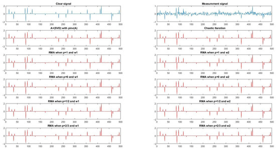
Figure 1. (m, n) = (250, 500).

Subsequently, we chose $A$ of large size $=5000, m=1000, n_{NZ}=50, r=500$. Corresponding to stochastic signals, the signal reconstructed by Iterative Figure 1 with ${\omega }_1$ and ${\omega }_1$ when $p=0$,1$,\frac{1}{2},\frac{2}{3}$, (4) based on $A^{+}$ (SVD) and Chaotic Iteration are displayed in Figure 2. The measurement signal $f$ is plotted in Figure 2, where $\sigma =0.5$. For two groups of parameters, we randomly chose some groups of different numerical experiments and listed the results in Table 1 and Table 2, respectively.

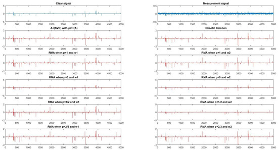
Figure 2. (m, n) = (1000, 5000).

Table 1. The comparison of ($m,n,rank(A),n_{NZ}$ ) = (250, 500, 200, 30).

	Algorithm	SNR	Time(s)	Algorithm	SNR	Time(s)
$\sigma =0$	$A^{+}$(SVD)	19.8251	0.044559	Chaotic	18.0157	0.028162
$I=2.5102$	ERMA${\omega }_{1, } p=1$	18.0113	0.027638	ERMA${\omega }_{2, } p=1$	32.5775	0.026196
$\alpha =1.6447\times {10}^{-6}$	ERMA${\omega }_{1,} p=0$	37.2878	0.027142	ERMA${\omega }_{2,} p=0$	40.1602	0.028243
$c=8.6203\times {10}^{15}$	ERMA${\omega }_{1,} p=1/2$	32.1598	0.031926	ERMA${\omega }_{2,} p=1/2$	37.0352	0.029582
	ERMA${\omega }_{1,} p=2/3$	36.0088	0.029953	ERMA${\omega }_{2,} p=2/3$	35.7393	0.032527
$\sigma =0.2$	$A^{+}$(SVD)	20.1438	0.044666	Chaotic	19.3884	0.026892
$I=2.3396$	ERMA${\omega }_{1,} p=1$	19.1838	0.029084	ERMA${\omega }_{2,} p=1$	32.4715	0.035649
$\alpha =1.7324\times {10}^{-6}$	ERMA${\omega }_{1,} p=0$	41.1679	0.032367	ERMA${\omega }_{2,} p=0$	43.0686	0.031641
$c=8.6203\times {10}^{-15}$	ERMA${\omega }_{1,} p=1/2$	29.1526	0.033237	ERMA${\omega }_{2,} p=1/2$	41.2370	0.035814
	ERMA${\omega }_{1,} p=2/3$	34.1705	0.047743	ERMA${\omega }_{2,} p=2/3$	39.1498	0.034877
$\sigma =0.5$	$A^{+}$(SVD)	19.0761	0.038465	Chaotic	18.3561	0.028174
$I=2.4999$	ERMA${\omega }_{1,} p=1$	18.3558	0.026806	ERMA${\omega }_{2,} p=1$	32.0254	0.029678
$\alpha =1.6235\times {10}^{-6}$	ERMA${\omega }_{1,} p=0$	32.0078	0.026468	ERMA${\omega }_{2,} p=0$	37.7192	0.027780
$c=7.9038\times {10}^{15}$	ERMA${\omega }_{1,} p=1/2$	28.1766	0.037457	ERMA${\omega }_{2,} p=1/2$	36.3582	0.033224
	ERMA${\omega }_{1,} p=2/3$	31.9909	0.033079	ERMA${\omega }_{2,} p=2/3$	35.4432	0.031825
$\sigma =0.8$	$A^{+}$(SVD)	14.6728	0.047050	Chaotic	14.5392	0.035564
$I=2.3549$	ERMA${\omega }_{1,} p=1$	14.5799	0.038262	ERMA${\omega }_{2,} p=1$	20.8947	0.040986
$\alpha =1.7534\times {10}^{-6}$	ERMA${\omega }_{1,} p=0$	21.5914	0.045155	ERMA${\omega }_{2,} p=0$	25.3924	0.039750
$c=8.2674\times {10}^{15}$	ERMA${\omega }_{1,} p=1/2$	18.4561	0.047157	ERMA${\omega }_{2,} p=1/2$	23.8044	0.060262
	ERMA${\omega }_{1,} p=2/3$	20.2264	0.042789	ERMA${\omega }_{2,} p=2/3$	23.0527	0.050048
$\sigma =1$	$A^{+}$(SVD)	11.9307	0.037875	Chaotic	11.4252	0.025827
$I=1.8277$	ERMA${\omega }_{1,} p=1$	11.4237	0.023979	ERMA${\omega }_{2,} p=1$	17.7616	0.026214
$\alpha =1.7001\times {10}^{-6}$	ERMA${\omega }_{1,} p=0$	20.4510	0.026325	ERMA${\omega }_{2,} p=0$	23.2305	0.027434
$c=8.3993\times {10}^{15}$	ERMA${\omega }_{1,} p=1/2$	16.2440	0.028772	ERMA${\omega }_{2,} p=1/2$	20.9194	0.031776
	ERMA${\omega }_{1,} p=2/3$	18.1365	0.031133	ERMA	19.9158	0.031347
$\sigma =2$	$A^{+}$(SVD)	11.8258	0.048401	Chaotic	11.6290	0.033802
$I=1.9283$	ERMA${\omega }_{1,} p=1$	11.6270	0.023583	ERMA${\omega }_{2,} p=1$	14.9244	0.039773
$\alpha =1.7534\times {10}^{-6}$	ERMA${\omega }_{1,} p=0$	14.7849	0.033782	ERMA${\omega }_{2,} p=0$	16.8113	0.035556
$c=8.0975\times {10}^{15}$	ERMA${\omega }_{1,} p=1/2$	14.3213	0.058803	ERMA${\omega }_{2,} p=1/2$	15.9718	0.035959
	ERMA${\omega }_{1,} p=2/3$	14.7800	0.047833	ERMA${\omega }_{2,} p=2/3$	15.6049	0.037541

Table 2. The comparison of ($m,n,rank(A),n_{NZ}$ ) = (1000, 5000, 500, 50).

	Algorithm	SNR	Time(s)	Algorithm	SNR	Time(s)
$\sigma =0$	$A^{+}$(SVD)	10.2378	3.848475	Chaotic	10.2579	3.582770
$I=0.4807$	ERMA${\omega }_{1,} p=1$	10.2579	3.380426	ERMA${\omega }_{2,} p=1$	14.9701	3.268581
$\alpha =6.3215\times {10}^{-8}$	ERMA${\omega }_{1,} p=0$	18.6892	3.704526	ERMA${\omega }_{2,} p=0$	20.4912	3.234485
$c=3.5619\times {10}^{16}$	ERMA${\omega }_{1,} p=1/2$	13.6919	3.545974	ERMA${\omega }_{2,} p=1/2$	17.8093	3.559504
	ERMA${\omega }_{1,} p=2/3$	15.2319	3.253955	ERMA${\omega }_{2,} p=2/3$	16.8820	3.266536
$\sigma =0.2$	$A^{+}$(SVD)	7.9981	3.700763	Chaotic	7.9993	3.221959
$I=0.4131$	ERMA${\omega }_{1,} p=1$	7.9993	3.222183	ERMA${\omega }_{2,} p=1$	11.2804	3.224178
$\alpha =5.9979\times {10}^{-8}$	ERMA${\omega }_{1, } p=0$	13.4954	3.214983	ERMA${\omega }_{2,} p=0$	15.2454	3.219813
$c=2.4434\times {10}^{16}$	ERMA${\omega }_{1,} p=1/2$	10.4032	3.224926	ERMA${\omega }_{2,} p=1/2$	13.2725	3.233614
	ERMA${\omega }_{1,} p=2/3$	11.4345	3.229159	ERMA${\omega }_{2,} p=2/3$	12.6096	3.217367
$\sigma =0.5$	$A^{+}$(SVD)	9.5544	3.733797	Chaotic	9.5565	3.371611
$I=0.4742$	ERMA${\omega }_{1,} p=1$	9.5565	3.226727	ERMA${\omega }_{2,} p=1$	14.5790	3.398832
$\alpha =6.1911\times {10}^{-8}$	ERMA${\omega }_{1,} p=0$	20.8740	3.333231	ERMA${\omega }_{2,} p=0$	21.6455	3.206791
$c=3.9381\times {10}^{16}$	ERMA${\omega }_{1,} p=1/2$	14.0289	3.885603	ERMA${\omega }_{2,} p=1/2$	18.0554	3.214479
	ERMA${\omega }_{1,} p=2/3$	16.1118	3.948218	ERMA${\omega }_{2,} p=2/3$	16.8428	3.228236
$\sigma =0.8$	$A^{+}$(SVD)	8.7799	3.788281	Chaotic	8.7916	3.194924
$I=0.4481$	ERMA${\omega }_{1,} p=1$	8.7917	3.211612	ERMA${\omega }_{2,} p=1$	12.8191	3.213434
$\alpha =5.9648\times {10}^{-8}$	ERMA${\omega }_{1,} p=0$	15.9546	3.200618	ERMA${\omega }_{2,} p=0$	17.6266	3.236925
$c=3.0408\times {10}^{16}$	ERMA${\omega }_{1,} p=1/2$	11.8424	3.214958	ERMA${\omega }_{2,} p=1/2$	15.1458	3.238623
	ERMA${\omega }_{1, } p=2/3$	13.1172	3.217332	ERMA${\omega }_{2,} p=2/3$	14.3617	3.219191
$\sigma =1$	$A^{+}$(SVD)	7.7927	3.767992	Chaotic	7.7971	3.313606
$I=0.4723$	ERMA${\omega }_{1,} p=1$	7.7971	3.196600	ERMA${\omega }_{2,} p=1$	11.0463	3.229021
$\alpha =6.1611\times {10}^{-8}$	ERMA${\omega }_{1,} p=0$	12.7602	3.212222	ERMA${\omega }_{2,} p=0$	14.3195	3.207623
$c=2.6591\times {10}^{16}$	ERMA${\omega }_{1,} p=1/2$	10.2262	3.220439	ERMA${\omega }_{2,} p=1/2$	12.6659	3.219741
	ERMA${\omega }_{1,} p=2/3$	11.0847	3.240974	ERMA${\omega }_{2,} p=2/3$	12.1478	3.214091
$\sigma =2$	$A^{+}$(SVD)	8.0947	3.701683	Chaotic	8.0938	3.190012
$I=0.4758$	ERMA${\omega }_{1,} p=1$	8.0938	3.191272	ERMA${\omega }_{2,} p=1$	11.9725	3.197868
$\alpha =6.2299\times {10}^{-8}$	ERMA${\omega }_{1,} p=0$	15.2115	3.200297	ERMA${\omega }_{2,} p=0$	17.0376	3.197985
$c=2.1860\times {10}^{16}$	ERMA${\omega }_{1,} p=1/2$	11.1243	3.210141	ERMA${\omega }_{2,} p=1/2$	14.3941	3.217404
	ERMA${\omega }_{1,} p=2/3$	12.3743	3.213414	ERMA${\omega }_{2,} p=2/3$	13.5538	3.216027

In Table 1 and Table 2, $c$is $cond(A)$ and $I$ is initial SNR. Obviously, these condition numbers of $A$ were large and initial SNR were small. Thus, solving problem (2) is very difficult. Comparing these data in Table 1 and Table 2, we can see the restored signals effected by (4) based on $A^{+}$(SVD) algorithm, Chaotic Iteration, ERMA with ${\omega }_1$ and ${\omega }_2$, and ERMA with ${\omega }_2$. When $p=0$, the SNR of ERMA with ${\omega }_2$ was the largest among all these results. Although the running times of these algorithms for one-dimensional signal reconstruction were small, it still can be seen that the running time of Chaotic Iteration, ERMA with ${\omega }_{1, } p=0$, and ERMA with ${\omega }_{2, } p=0$ were almost the same, and the time consumed by the (4) based on $A^{+}$ (SVD) algorithm was bigger than those consumed by the above three algorithms. This is because the formula of (4) involves computing the SVD decomposition, and the remaining algorithms just use matrix-vector product. Thus, as we can predict, the relationship of computing time was ERMA with ${\omega }_{2, } p=0\approx$ ERMA with ${\omega }_{2, } p=0\approx$ Chaotic Iteration < (4) based on $A^{+}$ (SVD) algorithm, and the relationship of SNR of all methods was ERMA with ${\omega }_{2, } p=0$> ERMA with ${\omega }_{1, } p=0$ > Chaotic Iteration $\approx$ (4) based on $A^{+}$ (SVD) algorithm.

When the above several algorithms were applied to image deblurring, the reconstructed results for $m<n(m=64,n=80)$ image convolved by a $7\times 7$ Gaussian kernel and for $m=n=256$ image convolved by $5\times 5$ disk kernel were found, as shown in Figure 3 and Figure 4, respectively. The first set of images was $m<n(64\times 80)$, which had a smaller scale and was not normal. The second set of images was $m=n(256\times 256)$, which was the common size. The choice of these two sizes of images illustrates the generality of our algorithm. We noticed that the ERMA algorithm had better performance than others. In Table 3 and Table 4, which listed results of Figure 3 and Figure 4, we discovered that the relationship of computing speed was ERMA Chaotic $\ll A^{+}$ (SVD), that of SNR and SSIM was $A^{+}$ (SVD) $\approx$ ERMA (${\omega }_{2, } p=0$) > ERMA(${\omega }_{1, } p=0$)(RMA-IF) > Chaotic (ERMA (${\omega }_{1, } p=0$)), and that of MSE was $A^{+}$ (SVD)$\approx$ ERMA (${\omega }_{2, } p=0$) $<$ ERMA(${\omega }_{1,} p=0$) (RMA-IF) $<$ Chaotic (ERMA (${\omega }_{1, } p=0$)). Obviously, the parameter of ${\omega }_{2, } p=0$ in ERMA is a better choice than others. We had no doubt that we obtained the same conclusion for image blurring with signal reconstruction.

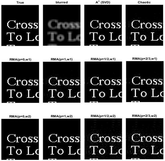
Figure 3. Deblurring results of the $A^{+}$ Bregman iteration, Chaotic iteration and RMA with ${\omega }_{1 }$, ${\omega }_{2 }$, when $p=0$,1$,1/2,2/3$ for a 64 × 80 part of the sparse Words image convolved by a $5\times 5$ Gaussian kernel and contaminated by a Gaussian white noise of ${\sigma }^2,\sigma =10$.

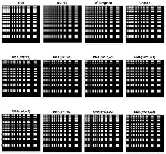
Figure 4. Deblurring results of the $A^T$ Bregman iteration, Chaotic iteration, and RMA with ${\omega }_{1 }$, ${\omega }_{2 }$, when $p=0$,1$,1/2,2/3$ for a 256 × 256 image convolved by a $5\times 5$ disk kernel.

Table 3. The comparison of Figure 3 deblurring results.

Algorithm	SNR	SSIM	MSE	Time(s)
$A^{+}$(SVD)	22.2237	0.997118	0.000490	46.163594
Chaotic	14.5435	0.859480	0.002639	0.144938
ERMA${\omega }_{1, } p=1$	14.5435	0.859480	0.002639	0.161000
ERMA${\omega }_{1, } p=0$	17.9619	0. 970449	0.001201	0.209249
ERMA${\omega }_{1, } p=1/2$	16.3457	0.932650	0.001743	0.301524
ERMA${\omega }_{1, } p=2/3$	15.7405	0.908980	0.002004	0.287078
ERMA${\omega }_{2, } p=1$	17.4646	0.958452	0.001347	0.156247
ERMA${\omega }_{2, } p=0$	20.8713	0.994342	0.000615	0.157634
ERMA${\omega }_{2, } p=1/2$	11.2449	0.661560	0.005641	0.233360
ERMA${\omega }_{2, } p=2/3$	11.5423	0.681532	0.005268	0.224610

Table 4. The comparison of Figure 4 deblurring results.

Algorithm	SNR	SSIM	MSE	Time(s)
$A^T$(SVD)	5.7618	0.632264	0.052809	2.204459
Chaotic	10.3730	0.762658	0.018263	4.705136
ERMA${\omega }_{1, } p=1$	10.3730	0.762658	0.018263	4.710400
ERMA${\omega }_{1, } p=0$	11.4374	0.898208	0.014296	4.748141
ERMA${\omega }_{1, } p=1/2$	10.9434	0.853082	0.016016	5.143209
ERMA${\omega }_{1, } p=2/3$	10.7377	0.823245	0.016793	5.102806
ERMA${\omega }_{2, } p=1$	11.0814	0.877404	0.015516	4.766557
ERMA${\omega }_{2, } p=0$	11.9192	0.912981	0.012798	4.733365
ERMA${\omega }_{2, } p=1/2$	9.8362	0.620787	0.020666	5.153214
ERMA${\omega }_{2, } p=2/3$	9.8840	0.634580	0.020440	5.146052

In fact, the complexity analysis included a comparison of the outcomes of several methods. $K$ was the same loop number as before. Thus, the workload of the $A^{+}$ algorithm (4) was divided into two parts. They are the workload of the $A^{+}$ and the loop of the (4). Because of the singular value decomposition including matrix multiplication and matrix and eigenvalue calculation, the workload was $O(n^3)$ when computing $A=USV$ and $A^{+}=V^T{S}^{+}{U}^T$ when $m<n$. Because the loop only involved matrix and vector multiplication, the workplace of the (4) loop was $O(m\times n\times K)$. As a result, the $A^{+}$ algorithm’s overall burden was $O(m\times n\times K)+O(n^3)$. The workload of the remaining algorithms was equal to $(m\times n\times K)$. Obviously, $K<m\ll n$, and the $A^{+}$ algorithm (4) had the most workload compared to the other three algorithms [23,26,27]. The calculation of the generalized inverse matrix $A^{+}$ was the main workload.

The comparison of the SNR, SSIM, and MSE data for all methods in Table 3 and Table 4 shows that ERMA outperformed other two methods and ${\omega }_{2, } p=0$ was a relatively good choice for our new algorithm, which was found to be more effective than the $A^{+}$(SVD), Chaotic algorithm in [26], and RMA-IF (that is, ERMA with ${\omega }_{1, } p=1$) in [27], given the enhanced sparsity proposed in this work. Such a parameter group can improve the calculation efficiency and keep the effectiveness of image recovery.

5. Conclusions

We have proposed an effective reweighted ${\ell }_1$ minimization algorithm. The algorithm is based on the Chaotic Iteration and iterative reweighted strategy that is used to solve the $\underset{u\in R^n}{\min }\{{||u||}_p^p:Au=f\}$ problem. ERMA is competitive due to its restored effectiveness and smaller workload in comparison to its initial version. Numerically and theoretically, ERMA not only inherits all merits of Chaotic Iteration and linearized Bregman iteration, but also greatly improves the SNR, SSIM, and MSE. Importantly, ERMA still preserves stable results when $A$ is a very ill condition. Overall, ERMA remains as a good alternative when the condition of $A$ is unknown and the measurement signal contains error.

References

- Aspandi, D.; Martinez, O.; Sukno, F.; Binefa, X. Composite recurrent network with internal denoising for facial alignment in still and video images in the wild. Image Vis. Comput. 2021, 111, 104189. [Google Scholar] [CrossRef]
- Zhu, P.; Jiang, Z.; Zhang, J.; Zhang, Y.; Wu, P. Remote sensing image watermarking based on motion blur degeneration and restoration model. Optics 2021, 248, 168018. [Google Scholar] [CrossRef]
- Chaudhari, A.; Kulkarni, J. Adaptive Bayesian Filtering Based Restoration of MR Images. Biomed. Signal Process. Control. 2021, 68, 102620. [Google Scholar] [CrossRef]
- Chen, S.S.; Donoho, D.L.; Saunders, M.A. Atomic Decomposition by Basis Pursuit. SIAM Journal on Scientific Computing 1998, 43(1), 129–159. [Google Scholar] [CrossRef]
- Wang, Y.; Yang, J.; Yin, W.; Zhang, Y. A New Alternating Minimization Algorithm for Total Variation Image Reconstruction. SIAM J. Imag. Sci. 2008, 1, 248–272. [Google Scholar] [CrossRef]
- Tsaig, Y.; Donoho, D.L. Extensions of compressed sensing. Signal Process. 2006, 86, 549–571. [Google Scholar] [CrossRef]
- Candes, E.J.; Romberg, J. Errata for Quantitative Robust Uncertainty Principles and Optimally Sparse Decompositions. Math. Ann. 2007, 7, 529–531. [Google Scholar] [CrossRef][Green Version]
- Candes, E.J.; Romberg, J.; Tao, T. Robust uncertainty principles: Exact signal reconstruction from highly incomplete frequency information. IEEE Trans. Inf. Theory 2006, 52, 489–509. [Google Scholar] [CrossRef]
- Misra, G.D.; Donoho, D.L. Compressed Sensing. IEEE Trans. Inf. Theory 2006, 52, 1289–1306. [Google Scholar]
- Zhang, X.; Zhang, S.; Lin, J.; Sun, F.; Zhu, X.; Yang, Y.; Tong, X.; Yang, H. An Efficient Seismic Data Acquisition Based on Compressed Sensing Architecture With Generative Adversarial Networks. IEEE Access 2019, 7, 105948–105961. [Google Scholar] [CrossRef]
- Shi, L.; Qu, G.; Wang, Q. A Method of Reweighting the Sensing Matrix for Compressed Sensing. IEEE Access 2021, 9, 21425–21432. [Google Scholar] [CrossRef]
- Xu, S.; Yang, X.; Jiang, S. A fast nonlocally centralized sparse representation algorithm for image denoising. Signal Process. 2017, 131, 99–112. [Google Scholar] [CrossRef]
- Xie, J.; Liao, A.; Lei, Y. A new accelerated alternating minimization method for analysis sparse recovery. Signal Process. 2018, 145, 167–174. [Google Scholar] [CrossRef]
- Cai, J.-F.; Osher, S.; Shen, Z. Linearized Bregman iterations for compressed sensing. Math. Comput. 2009, 78, 1515–1536. [Google Scholar] [CrossRef]
- Cholamjiak, W.; Khan, S.A.; Yambangwai, D.; Kazmi, K.R. Strong Convergence Analysis of Common Variational Inclusion problems Involving an Inertial Parallel Monotone Hybrid Method for a Novel Application to Image Restoration. RACSAM 2020, 114, 99. [Google Scholar] [CrossRef]
- Cholamjiak, W.; Dutta, H.; Yambangwai, D. Image Restorations Using an Inertial Parallel Pybrid Algorithm with Armijo Linesearch for Nonmonotone Equilibrium Problems. Chaos Solitons Fractals 2021, 153, 111462. [Google Scholar] [CrossRef]
- Suantai, S.; Peeyada, P.; Yambangwai, D.; Cholamjiak, W. A Parallel-Viscosity-Type Subgradient Extragradient-Line Method for Finding the Common Solution of Variational Inequality Problems Applied to Image Restoration Problems. Mathematics 2020, 8, 248. [Google Scholar] [CrossRef]
- Yambangwai, D.; Khan, S.A.; Dutta, H.; Cholamjiak, W. Image Restoration by Advanced Parallel Inertial Forward–Backward Splitting Methods. Soft Comput. 2021, 25, 6029–6042. [Google Scholar] [CrossRef]
- Cai, J.F.; Shen, S.O. Convergence of the Linearized Bregman Iteration for ℓ1-norm Minimization. Math. Comput. 2009, 78, 2127–2136. [Google Scholar] [CrossRef]
- Amaral, G.; Calliari, F.; Lunglmayr, M. Profile-Splitting Linearized Bregman Iterations for Trend Break Detection Applications. Electronics 2020, 9, 423. [Google Scholar] [CrossRef]
- Osher, S.; Mao, Y.; Dong, B.; Yin, W. Fast Linearized Bregman Iteration for Compressive Sensing and Sparse Denoising: UCLA. Commun. Math. Sci. 2010, 8, 93–111. [Google Scholar]
- Cai, J.; Osher, S.; Shen, Z. Linearized Bregman Iterations for Frame-Based Image Deblurring. SIAM J. Imaging Sci. 2009, 2, 226–252. [Google Scholar] [CrossRef]
- Qiao, T.; Li, W.; Wu, B. A New Algorithm Based on Linearized Bregman Iteration with Generalized Inverse for Compressed Sensing. Circuits Syst. Signal Process. 2014, 33, 1527–1539. [Google Scholar] [CrossRef]
- Liu, J.; Ma, R.; Zeng, X.; Liu, W.; Wang, M.; Chen, H. An efficient non-convex total variation approach for image deblurring and denoising. Appl. Math. Comput. 2021, 397, 125977. [Google Scholar] [CrossRef]
- Liu, J.; Ni, A.; Ni, G. A nonconvex l1(l1−l2) model for image restoration with impulse noise. J. Comput. Appl. Math. 2020, 378, 112934. [Google Scholar] [CrossRef]
- Qiao, T.; Li, W.; Wu, B.; Wang, J. A chaotic iterative algorithm based on linearized Bregman iteration for image deblurring. Inf. Sci. 2014, 272, 198–208. [Google Scholar] [CrossRef]
- Qiao, T.; Wu, B.; Li, W.; Dong, A. A new reweighted l 1 minimization algorithm for image deblurring. J. Inequalities Appl. 2014, 2014, 238. [Google Scholar] [CrossRef]
- Rose, K. Deterministic annealing for clustering, compression, classification, regression, and related optimization problems. Proc. IEEE 1998, 86, 2210–2239. [Google Scholar] [CrossRef]
- Jin, D.; Yang, Y.; Ge, T.; Wu, D. A Fast Sparse Recovery Algorithm for Compressed Sensing Using Approximate l0 Norm and Modified Newton Method. Materials 2019, 12, 1227. [Google Scholar] [CrossRef]
- Materassi, D.; Innocenti, G.; Giarré, L.; Salapaka, M. Model Identification of a Network as Compressing Sensing. Syst. Control. Lett. 2013, 62, 664–672. [Google Scholar] [CrossRef]
- Zhou, F.; Wu, Y.; Dai, Y.; Wang, P. Detection of Small Target Using Schatten 1/2 Quasi-Norm Regularization with Reweighted Sparse Enhancement in Complex Infrared Scenes. Remote Sens. 2019, 11, 2058. [Google Scholar] [CrossRef]
- Zhu, H.; Xiao, Y.; Wu, S.-Y. Large sparse signal recovery by conjugate gradient algorithm based on smoothing technique. Comput. Math. Appl. 2013, 66, 24–32. [Google Scholar] [CrossRef]
- Xiu, X.; Kong, L.; Yan, H. Iterative Reweighted Methods for l1–lp Minimization. Comput. Optim. Appl. 2018, 70, 201–219. [Google Scholar] [CrossRef]
- Faris, H.; Mafarja, M.M.; Heidari, A.A.; Aljarah, I.; Al-Zoubi, A.; Mirjalili, S.; Fujita, H. An efficient binary Salp Swarm Algorithm with crossover scheme for feature selection problems. Knowl.-Based Syst. 2018, 154, 43–67. [Google Scholar] [CrossRef]
- Abdi, M.J. Comparison of Several Reweighted l1-Algorithms for Solving Cardinality Minimization Problems. Mathematics 2013, arXiv:1304.6655. [Google Scholar]
- Qiao, D.; Pang, G.K.H. An Iteratively Reweighted Least Square Algorithm for RSS-Based Sensor Network Localization; IEEE: Beijing, China, 2011; pp. 1085–1092. [Google Scholar]
- Daubechies, I.; DeVore, R.; Fornasier, M.; Güntürk, C.S. Iteratively reweighted least squares minimization for sparse recovery. Commun. Pure Appl. Math. 2010, 63, 1–38. [Google Scholar] [CrossRef]
- Cao, W.; Sun, J.; Xu, Z. Fast Image Deconvolution Using Closed-form Thresholding Formulas of Lq(q = 12, 23) Regularization. J. Vis. Commun. Image Represent. 2013, 24, 31–41. [Google Scholar] [CrossRef]
- Zhang, H.; Cheng, L.Z. A− Linear Bregman Iterative Algorithm. Comput. Math. 2010, 32, 97–104. [Google Scholar]
Publisher’s Note: MDPI stays neutral with regard to jurisdictional claims in published maps and institutional affiliations. |
© 2021 by the authors. Licensee MDPI, Basel, Switzerland. This article is an open access article distributed under the terms and conditions of the Creative Commons Attribution (CC BY) license (https://creativecommons.org/licenses/by/4.0/).