Computing a Group of Polynomials over a Galois Field in FPGA Architecture

Abstract

For the most extensive range of tasks, such as real-time data processing in intelligent transport systems, etc., advanced computer-based techniques are required. They include field-programmable gate arrays (FPGAs). This paper proposes a method of pre-calculating the hardware complexity of computing a group of polynomial functions depending on the number of input variables of the said functions, based on the microchips of FPGAs. These assessments are reduced for a group of polynomial functions due to computing the common values of elementary polynomials. Implementation is performed using similar software IP-cores adapted to the architecture of user-programmable logic arrays. The architecture of FPGAs includes lookup tables and D flip-flops. This circumstance ensures that the pipelined data processing provides the highest operating speed of a device, which implements the group of polynomial functions defined over a Galois field, independently of the number of variables of the said functions. A group of polynomial functions is computed based on common variables. Therefore, the input/output blocks of FPGAs are not a significant limiting factor for the hardware complexity estimates. Estimates obtained in using the method proposed allow evaluating the amount of the reconfigurable resources of FPGAs, required for implementing a group of polynomial functions defined over a Galois field. This refers to both the existing FPGAs and promising ones that have not yet been implemented.

1. Introduction

To ensure the seamless operation of intelligent transport systems (ITSes), it is required to process large amounts of monitoring information of various formats, purposes, and confidentiality levels in the real-time mode [1,2,3]. General- and special-purpose computing machinery is essential to information processing. Computer hardware (CHW) can be speeded up in two ways. The first one is extensive, requiring continuously enhancing computational capacities and developing special-purpose CHW focused on a predefined scope of tasks. The second one is intensive, requiring a flexible adaptation of the CHW hardware to a certain task, particularly rejecting the classical, von Neumann’s, CHW common-bus architecture. Unlike the former, the latter way allows implementing devices with higher speeds than that for general-purpose CHW. Examples of special purpose computing devices that use field-programmable gate arrays (FPGAs) [4] are given in [5,6]. Using high-speed CHW devices that allow implementing various algorithms of distributed data processing at different times is relevant in solving various ITS-related tasks, such as data processing in large databases [7], analysis of discrete Markovian processes [8,9], nonlinear filtering of data [10], etc.

To solve the above scope of problems, FPGAs [4] can be used that include reconfigurable logical elements, i.e., lookup tables (LUTs(x)), D flip-flops, and input/output blocks (IOBs). In [11,12,13], an approach is presented based on reducing the problem of processing data arrays (exemplified by maps) to implementing similar FPGA-based operations. Several studies [14,15,16] show that the problem of implementing arbitrary maps of one set of elements into another set is reduced to the distributed computation of a group of nonlinear polynomial functions (polynomials, functions) of a given number of variables defined over a Galois field $GF(2^k)$ of a certain power [17]. A cooperative distributed FPGA-based computation method is proposed for the said polynomials. We obtained the estimates of hardware complexity for a group of polynomials by the number of reconfigurable FPGA elements. It is shown that the computations of elementary polynomials common for the functions from the set to be implemented considerably save the reconfigurable logical resources of FPGA. Due to the pipelined implementation of computing a group of functions based on similar IP-cores, estimates of operation delays of pipeline devices computing the set of polynomials on FPGA are weakly dependent on the number of variables at the input of these functions.

The article is contained three basic Sections: (1) Basic Terms and Definitions; (2) Hardware Complexity of Implementing a Group of Polynomials in the FPGA Architecture and (3) Discussion. In Section 1, the concept of a polynomial of m variables and operations on elements of the Galois field is introduced in accordance with [17]. Statements are made regarding the hardware and time complexity of the pipeline implementation of operations on elements of the Galois field in the FPGA architecture. The concept of a similar IP-core corresponding to FPGA architecture is introduced [16]. According to [14,15,16], the separate computation of a group of polynomials involves multiple recomputations of partial polynomial functions common to a group of polynomials. This significantly increases the complexity estimates by the number of such IP-cores. Section 2 presents and theoretically supports representing a group of polynomials over a Galois field. Estimates of the complexity of the implementation of this group by the number of similar IP cores are calculated. The proportion of IP-cores required to calculate parts of elementary polynomial functions common to a group of polynomials is determined. Section 3 defines the possibilities for using the proposed method to evaluate the characteristics of a group of polynomials (the number of variables and polynomials, the dimension of the Galois field) that are acceptable for implementation on a given FPGA-devices, both for existing and prospective.

2. Basic Terms and Definitions

Let us define a polynomial of m variables over a Galois field represented as $GF(2^k)$ [17]

$$f(x_1, \dots , x_m)={\displaystyle \sum _{i_1=0}^r\cdots {\displaystyle \sum _{i_m=0}^r{a}_{i_1\dots i_m}{x}_1^{i_1}·\dots ·x_m^{i_m}}}.$$

(1)

By defining the values of an m-dimensional matrix of coefficients $A=\left(a_{i_1\dots i_m}\right)$, $r=2^k-1$. Symbol $\mathsf{\Sigma }$ in (1) means the bitwise sum of elementary modulo-2 polynomials $a_{i_1\dots i_m}{x}_1^{i_1}·\dots ·x_m^{i_m}$, $i_j=\overline{0, r}$.

A polynomial function of the form (1) is representable as a self-similar formula: $f(x_1, \dots , x_m)={\displaystyle \sum _{i_1=0}^r{x}_1^{i_1}{\tilde{f}}_{i_1}(x_2, \dots , x_m)}$, where ${\tilde{f}}_{i_1}(x_2, \dots , x_m)$ is a function of $m-1$ variables defined according to (1).

Example 1.

Let for (1)$m=2$and$k=2$the elements of$GF(2^2)$be representable in both exponential$\left(\begin{array}{cccc}0& \xi & {\xi }^2& 1\end{array}\right)$and vector$\left(\begin{array}{cccc}\left(00\right)& \left(10\right)& \left(11\right)& \left(01\right)\end{array}\right)$forms equivalent to each other; the multiplication operation over the elements of$GF(2^2)$is defined as${\xi }^a{\xi }^b={\xi }^{\left(a+b\right)\mathrm{mod}3}$, and the addition operation is defined as the bitwise sum of elementary modulo-2 [17]. $f(x_1, x_2)={\displaystyle \sum _{i_1=0}^3{x}_1^{i_1}{\tilde{f}}_{i_1}(x_2)}={\displaystyle \sum _{i_1=0}^3{x}_1^{i_1}\left(a_{i_1, 0}+a_{i_1, 1}{x}_2^{}+a_{i_1, 2}{x}_2^2+a_{i_1, 3}{x}_2^3\right)}$ The coefficients of this polynomial are given by a two-dimensional matrix $A=\left(a_{i_1{i}_2}\right)=\left(\begin{array}{cccc}\xi & 0& 0& {\xi }^2\\ 1& 0& \xi & 0\\ 0& {\xi }^2& 0& 1\\ 1& 1& 0& 0\end{array}\right)$. Then $f(x_1, x_2)=\left(\xi +{\xi }^2{x}_2^3\right)+x_1^{}\left({\xi }^2{x}_2^{}+\xi x_2^2\right)+x_1^2\left({\xi }^2{x}_2^{}+x_2^3\right)+x_1^3\left(1+x_2^{}\right)$, and the values $f(0, 0)=\xi$, $f({\xi }^2, 0)=0$, $f(0, {\xi }^2)=1$.

Let us consider a polynomial represented as (1) on FPGA. According to [14], let us introduce the following statements:

Statement 1.

k LUTs (x),$x\ge 2k$, allow performing the following operations: raising to power i,$i=\overline{1, r}$, and multiplying two elements of$GF(2^k)$; multiplying two elements of$GF(2^k)$by a constant, followed by addition; and bitwise modulo-2 sum operation for x elements of$GF(2^k)$.

Statement 2.

The basic element for implementing a polynomial represented as (1) on FPGA is an IP-core that includes k LUTs (x),$x\ge 2k$, and k D flip-flops.

Statement 2 defines the hardware complexity of the basic element by the number of the programmable FPGA elements, i.e., k LUTs (x) and k D flip-flops, respectively. The pipelined operation delay time of a device implemented on these moduli does not depend on the number of variables of polynomial (1) and is defined by formula:

$$T=t_D+t_{IC}+\max \left(t_{in}, t_{\mathrm{LUT}(x)}, t_{out}\right),$$

(2)

where $t_D$, $t_{IC}$, and $t_{\mathrm{LUT}(x)}$ are operation delay times of D flip-flops, interconnections, and LUTs (x) for a given FPGA, while $t_{in}$ and $t_{out}$ are the delay times of IOBs that function to information input/output within the package of a given FPGA, respectively. Delay time of interconnections, $t_{IC}$, is computed for a given device using a particular computer-aided design system. Such as Vivado 2020.1 CAD system (Xilinx, Inc., San Jose, CA, USA), Quartus II (Intel, Inc., Santa Clara, CA, USA), etc.

For example, according to [4], for FPGA Virtex UltraScale, device XCVU065, in formula (2) operation delay time $t_D$, is 2.36 ns. $t_{in}$ and $t_{out}$ are equal to approximately 0.42 ns and 0.66 ns. The value of the value $t_{\mathrm{LUT}(x)}$ (x = 6) is less than the values $t_{in}$ and $t_{out}$. According to [15,18], the interconnections’ delay time does not exceed 70% of the total delay time of operation. As a result, according to (2), the upper bound of pipelined operation delay time of XCVU065 device is $2.36+\left(2.36+0.66\right)·0.7+0.66=5.134$ ns.

Problem of implementing a broad class of digital CHW devices is reduced to the problem of implementing an arbitrary map of the elements of set $F_1$ into set $F_2$. In [15], it is shown that, in case of $\left|F_1\right|\le {\left(2^k\right)}^m$, $\left|F_2\right|\le {\left(2^k\right)}^E$, this map can be represented by E polynomials of m variables over Galois field represented as $GF(2^k)$.

3. Hardware Complexity of Implementing a Group of Polynomials in the FPGA Architecture

According to Statement 1, let us find the hardware complexity estimates of implementing a group of E polynomials represented as (1) of m variables over the field $GF(2^k)$. Each of E polynomials represented as (1), generally speaking, is computed when using ${\left(2^k\right)}^m$ identical elementary polynomials. Let us introduce the following definitions of subsets of this set:

Definition 1.

First subset of elementary polynomials, power$Z_{1-E}$, includes elementary polynomials that are not used in computing each of E polynomials$f_1$, …,$f_E$because of multiplying it by the zero coefficient of matrix$A^{(e)}=\left(a_{i_1\dots i_m}^{(e)}\right)$, $e=\overline{1, E}$.

Definition 2.

First subset of elementary polynomials is divided into non-overlapping subsets, power$Z_{1-E}^{(j)}$, including elementary polynomials of j variables, $j=\overline{1, m}$, $Z_{1-E}={\displaystyle \sum _{j=1}^m{Z}_{1-E}^{(j)}}$.

Definition 3.

Each of E subsets of elementary polynomials, power$Z_e$, that are not overlapped with the first subset include elementary polynomials that are not used in computing$f_e$because of multiplying it by the zero coefficient of matrix$A^{(e)}=\left(a_{i_1\dots i_m}^{(e)}\right)$, $e=\overline{1, E}$.

A method is proposed to compute the hardware complexity estimates for a group of E polynomials of m variables represented (1) in the FPGA architecture. The method includes three stages:

Stage 1. Computing common elementary polynomials, among which there are at most $r^m$ of m variables and at most $r^{m-j}{C}_m^{m-j}$ of $\left(m-j\right)$ variables, $j=\overline{1, m}$.

Stage 2. Obtaining the values of the products of elementary polynomials and nonzero constants $A^{(e)}=\left(a_{i_1\dots i_m}^{(e)}\right)$, $e=\overline{1, E}$.

Stage 3. Bitwise modulo-2 addition of values obtained at Stage 2.

Let us define the hardware complexity estimates for computing a group of E polynomials represented as (1) in the FPGA architecture in using the basic elements, IP-cores, based on Statements 1 and 2. Due to the fact that the said IP-cores form a pipeline, operation delay time estimates do not practically depend on the number of variables m of each of E polynomials. The number of basic elements required at Stages 1, 2, and 3 is defined according to formulas:

$$N_1={\displaystyle \sum _{j=0}^{m-1}\left(\left(m-j-1\right)r^{m-j}{C}_m^{m-j}-Z_{1-E}^{(j)}\right)}$$

$$N_2={\displaystyle \sum _{e=1}^E\left]\left({\left(2^k\right)}^m-Z_e\right)/2\right[}={\displaystyle \sum _{e=1}^E{N}_2^{(e)}}$$

$$N_3={\displaystyle \sum _{e=1}^E\left]N_2^{(e)}/x\right[}, x\ge 2k.$$

Values of $Z_{1-E}^{(j)}$ and $Z_e$, $j=\overline{1, m}$, $e=\overline{1, E}$, are defined in accordance with the definitions 1–3. The total number of IP cores required to compute a group of E polynomials represented as (1) is:

$$N_{EP}=N_1+N_2+N_3.$$

(3)

Based on definitions 1–3 and the above true is the Theorem 1.

Theorem 1.

Hardware complexity of computing a group of E polynomials represented as (1) of m variables over$GF(2^k)$in the FPGA architecture by the number of IP-cores is calculated according to (3), the operation time delay was estimated according to (2), while the number of FPGA pins is defined as$k(m+E)$.

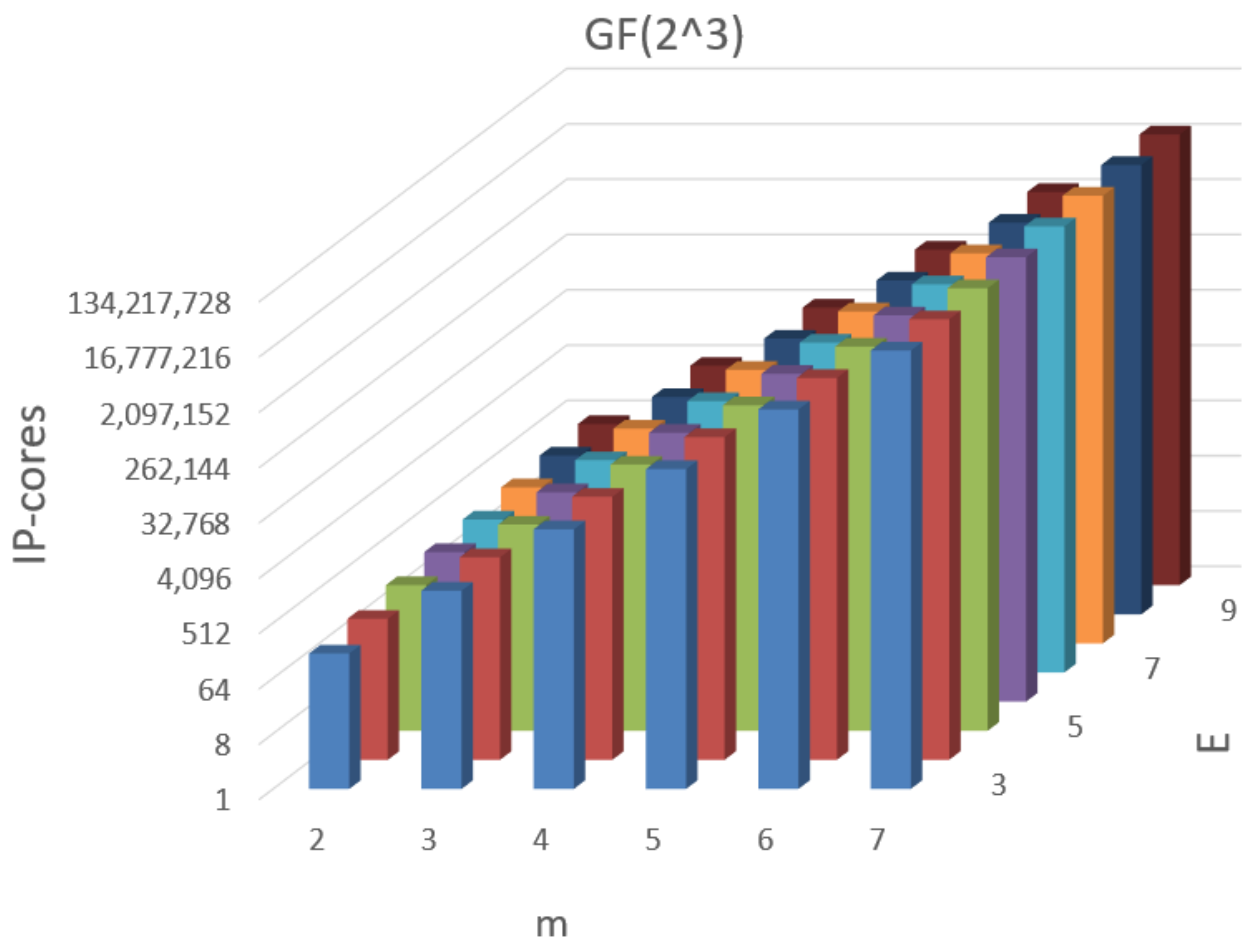
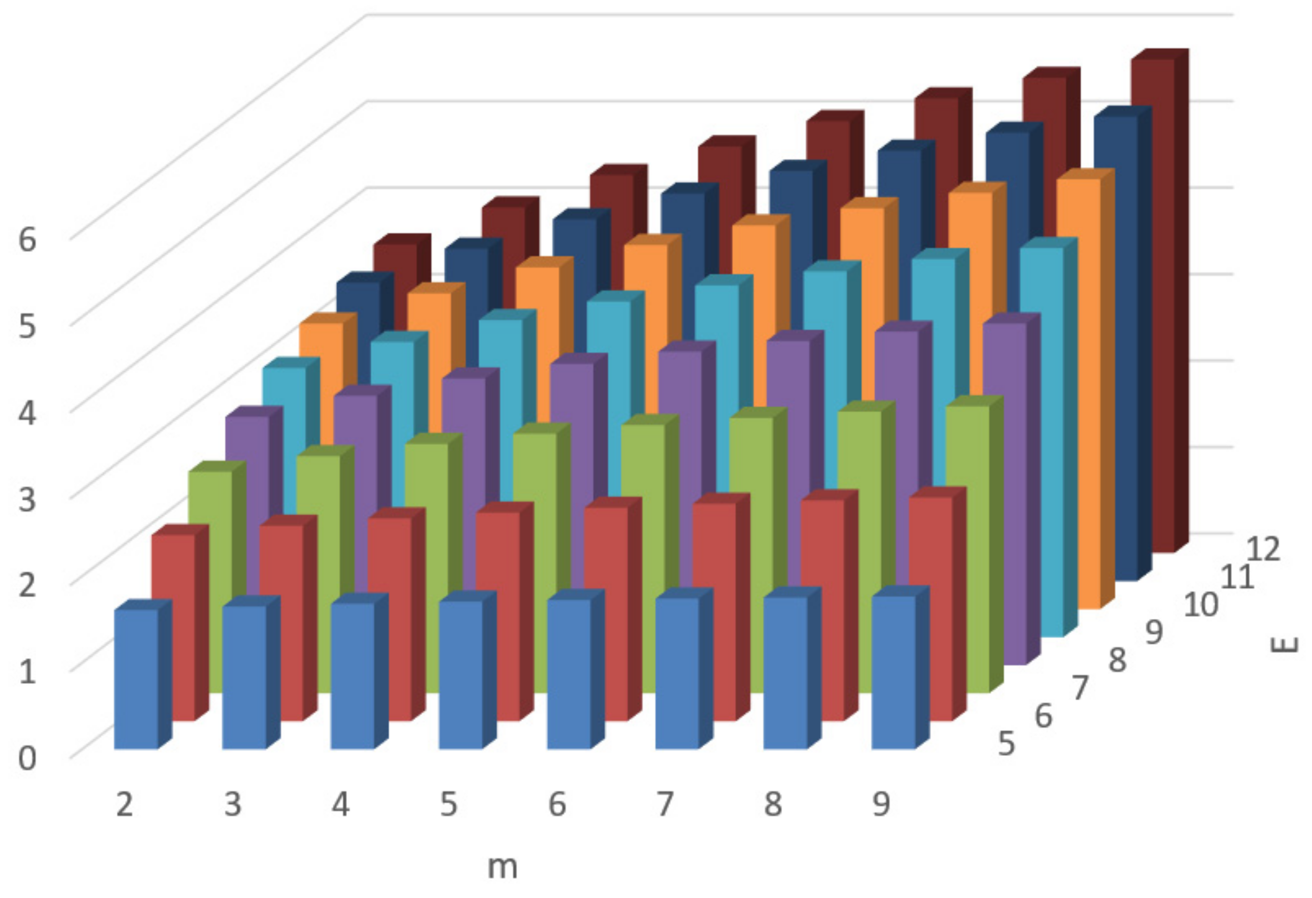
Let us analyze the hardware complexity estimates of implementing a group of polynomials in the FPGA architecture. Figure 1 and Figure 2 represent diagrams that show the dependency of the total number of IP-cores, $N_{EP}$, for a group of polynomials represented as (1) over $GF(2^2)$ and $GF(2^3)$, respectively, on the number of variables m and on the power of a group of polynomials E. According to the data given in Figure 1, the spread of estimates of the number of IP-cores for a group of polynomials represented as (1) over $GF(2^2)$ varies from 59 (m = 2, E = 5) to approximately $3.44·{10}^6$ (m = 9, E = 12). For a group implemented over $GF(2^2)$ (see Figure 2) these estimates range from 163 (m = 2, E = 5) to approximately $23.0·{10}^6$ (m = 7, E = 10). With the increase in the number of the variables of polynomials, an exponential increase in the estimate, $N_{EP}$, is observed, while the growth of E results in the practically linear increase in this estimate.

Of interest is also the contribution of the hardware complexity estimates for computing elementary polynomials common for each of E functions of $N_1$ to the total complexity estimate, $N_{EP}$. According to diagrams shown in Figure 3 and Figure 4, linear growth of the $N_1/N_{EP}$ ratio is observed in increasing the number of variables. However, the higher the value of E, the slower $N_1/N_{EP}$ grows. This observation is true for both $GF(2^2)$ and $GF(2^3)$. This is explained by the fact that the number of IP-cores required for computing elementary polynomials increases exponentially with the linear increase in the number of variables m.

The value $N_1/N_{EP}$ shows what effect will be in the case of the implementation of a group of E polynomials according to the proposed method compared with the separate implementation of each of their E polynomials over $GF(2^2)$ and $GF(2^3)$. For $GF(2^2)$ (see Figure 3) the spread of values of magnitude $N_1/N_{EP}$ varies from 15.3% (m = 2, E = 5) to 42.8% (m = 9, E = 12). For $GF(2^2)$ (see Figure 3)—from 30.1% (m = 2, E = 5) to 46.8% (m = 7, E = 10).

According to [15], implementing the given system from E polynomials of m variables over $GF(2^k)$ on one FPGA microcircuit is allowed, provided that the following conditions are met:

$$\left\{\begin{array}{l}{N}_{\mathrm{LUT}\left(\mathrm{x}\right)}\le k_{\mathrm{LUT}\left(\mathrm{x}\right)}·Q_{\mathrm{LUT}\left(\mathrm{x}\right)}\\ N_{\mathrm{D}}\le k_{\mathrm{D}}·Q_{\mathrm{D}}\\ N_{\mathrm{IOB}}\le k_{\mathrm{IOB}}·Q_{\mathrm{IOB}}\end{array}\right.,$$

(4)

where $N_{\mathrm{LUT}\left(\mathrm{x}\right)}$, $N_{\mathrm{D}}$, and $N_{\mathrm{IOB}}$ are the number of reconfigurable resources, LUTs(x), D flip-flops, and IOBs, respectively, required for implementing a group of E polynomials of m variables; $Q_{\mathrm{LUT}\left(\mathrm{x}\right)}$, $Q_{\mathrm{D}}$, and $Q_{\mathrm{IOB}}$ are the number of similar resources available to the user within the given FPGA, while $k_{\mathrm{LUT}\left(\mathrm{x}\right)}$, $k_{\mathrm{D}}$, and $k_{\mathrm{IOB}}$ are the use factors of the said reconfigurable resources.

Example 2.

Joint implementation of a group of two polynomials,$f^{(1)}(x_1, x_2)$and$f^{(2)}(x_1, x_2)$, having the structure given in Example 1, and given by the matrices of coefficients$A^{(1)}=\left(\begin{array}{cccc}\xi & 0& 0& {\xi }^2\\ 1& 0& \xi & 0\\ 0& {\xi }^2& 0& 1\\ 1& 1& 0& 0\end{array}\right)$and$A^{(2)}=\left(\begin{array}{cccc}1& 1& 0& 0\\ \xi & 0& {\xi }^2& 0\\ \xi & \xi & 0& 0\\ 0& \xi & 1& 0\end{array}\right)$. The implementation of step 1 of the proposed method is represented in the form of a two-dimensional matrix:$\left(\begin{array}{cccc}1& x_2^{}& -& x_2^3=1\\ x_1^{}& -& x_1^{}{x}_2^2& -\\ x_1^2& x_1^2{x}_2^{}& -& x_1^2·1\\ x_1^3=1& 1·x_2^{}& 1·x_2^2& -\end{array}\right)$. Five elementary polynomials do not need to be calculated, since the coefficients for them and in$f^{(1)}(x_1, x_2)$and in$f^{(2)}(x_1, x_2)$are zero; according to the definition of 2,$Z_{1-E}^{(0)}=1$,$Z_{1-E}^{(1)}=2$,$Z_{1-E}^{(2)}=Z_{1-E}^{(3)}=1$; for any value$x_j\in GF(2^2)$ $x_j^3=1$, therefore, it is not necessary to raise to the power of$x_j$,$j=\overline{1, 2}$. The result of stage 2 for each of the polynomials$f^{(1)}(x_1, x_2)$and$f^{(2)}(x_1, x_2)$is represented as matrices:$\left(\begin{array}{cccc}\xi & 0& -& {\xi }^2\\ x_1^{}& -& \xi x_1^{}{x}_2^2& -\\ 0& {\xi }^2{x}_1^2{x}_2^{}& -& x_1^2\\ 1& x_2^{}& 0& -\end{array}\right)$and$\left(\begin{array}{cccc}1& x_2^{}& -& 0\\ \xi x_1^{}& -& {\xi }^2{x}_1^{}{x}_2^2& -\\ \xi x_1^2& \xi x_1^2{x}_2^{}& -& 0\\ 0& \xi x_2^{}& x_2^2& -\end{array}\right)$, respectively, for which$Z_1=Z_2=3$(see Definition 3). Stage 3 consists of the bitwise addition of elementary polynomials and constants represented in the specified matrices:

$$f^{(1)}(x_1, x_2)=\xi +{\xi }^2+x_1+\xi x_1{x}_2^2+{\xi }^2{x}_1^2{x}_2+x_1^2+1+x_2=x_1+\xi x_1{x}_2^2+{\xi }^2{x}_1^2{x}_2+x_1^2+x_2,$$

$$f^{(2)}(x_1, x_2)=1+x_2+\xi x_1+{\xi }^2{x}_1{x}_2^2+\xi x_1^2+\xi x_1^2{x}_2+\xi x_2+x_2^2$$

4. Discussion

What is the advantage of the proposed approach to the implementation of a group of polynomials over a Galois field? Let us return to formula (3). Suppose the elements of this group of E polynomials are calculated separately. In that case, the hardware complexity will be defined as $N_{EP}^S=E·N_1+N_2+N_3$, that is, the value of $N_1$ will be increased by E times. As a result, the assessment of the complexity $N_{EP}^{}$ of the joint implementation of a group of E polynomials over a Galois field in comparison with their separate implementation $N_{EP}^S$ will be reduced in time.

$$N_{EP}^S/N_{EP}^{}=1+\left(E-1\right)N_1/N_{EP}^{}$$

(5)

The value $N_1/N_{EP}^{}$ is given for a group of E polynomials over a Galois field $GF(2^2)$ and $GF(2^3)$ given m and E on Figure 3 and Figure 4, respectively. By analogy, the estimate (5) has a range of values for $GF(2^2)$ from 1.61 (m = 2, E = 5) to 5.71 (m = 9, E = 12) and for $GF(2^3)$ from 1.90 (m = 2, E = 3) to 5.68 (m = 7, E = 9). These estimates are shown in Figure 5 and Figure 6.

For example, let us consider the FPGA XC7V585T of the Virtex-7 family. This FPGA includes 585,720 LUTs (6), 728,400 D flip-flops, and 850 IOBs. Use factors of each of the reconfigurable elements specified are 0.5. According to Theorem 1, FPGA-based implementation of a group of E polynomials of m variables over $GF(2^2)$ requires $2(m+E)$ IOBs, while that over $GF(2^3)$ requires $3(m+E)$ IOBs. According to Statement 1, implementing each IP-core over the elements of $GF(2^2)$ requires two LUTs (6) and two D flip-flops, while implementing over $GF(2^3)$ requires three LUTs (6) and three D flip-flops each. According to inequality (4) and formula (3), it is possible to implement on one FPGA XC7V585T the groups of, at most:

• Seven polynomials of seven variables over $GF(2^2)$, which correspond with mapping set $F_1: \left|F_1\right|\le 2^{14}$ into set $F_2: \left|F_2\right|\le 2^{14}$;
• 51 polynomials of six variables over $GF(2^2)$, which correspond with mapping set $F_1: \left|F_1\right|\le 2^{12}$ into set $F_2: \left|F_2\right|\le 2^{102}$; and
• 36 polynomials of four variables over $GF(2^3)$, which correspond with mapping set $F_1: \left|F_1\right|\le 2^{12}$ into set $F_2: \left|F_2\right|\le 2^{108}$.

In all the above cases of implementing the maps on FPGA XC7V585T, the limiting factor is the number of reconfigurable LUTs (6).

The proposed method allows us to estimate for a given group of E polynomials defined over $GF(2^k)$ and from m variables each the possibility of its implementation on a given FPGA-device. The degree of the field $GF(2^k)$, $k=2, 3$, is determined with reference to the features of existing FPGA-devises that implement LUT(4) and LUT(6) (see. Statement 1). The proposed method allows us to perform a similar study for any FPGA, both for existing and prospective.

5. Conclusions

Using the method proposed, we obtained the hardware complexity estimates for the distributed computation of a group of E polynomials of m variables over field $GF(2^k)$. Based on the above estimates, the values of E and m, can be defined. This group of polynomials can be implemented on an FPGA with the predefined characteristics by the number of reconfigurable elements available to the user. The method suits for estimating the hardware complexity of implementing a group of polynomials on both the existing and promising would-be FPGAs.

In arranging a pipeline, the average estimate of the operating delay of a device implementing the FPGA-based computation of a group of polynomials is weakly dependent on the power of a group of polynomials and on the number of their variables at the input. Due to the cooperative computing of polynomials from the group, the logical resources of FPGA are saved considerably. A relatively small set of elements, defined by input variables that are common for a group of polynomials, can be mapped in quite a large output set of values, the power of which exceeds considerably that of the input set.

The technique presented herein is a tool that allows the FPGA-based implementation of a frantic way to increase the data array processing speed in using the focused hardware basis. Due to reconfigurable elements available in the FPGA architecture, different maps of one set into another one can be implemented at different time intervals. This result is relevant in developing a hardware platform of intelligent transport systems, the role of which becomes increasingly important in the modern information society.