A Note on New Construction of Meyer-König and Zeller Operators and Its Approximation Properties

Abstract

The topic of approximation with positive linear operators in contemporary functional analysis and theory of functions has emerged in the last century. One of these operators is Meyer–König and Zeller operators and in this study a generalization of Meyer–König and Zeller type operators based on a function $\tau$ by using two sequences of functions will be presented. The most significant point is that the newly introduced operator preserves $\{1,\tau ,{\tau }^2\}$ instead of classical Korovkin test functions. Then asymptotic type formula, quantitative results, and local approximation properties of the introduced operators are given. Finally a numerical example performed by MATLAB is given to visualize the provided theoretical results.

1. Introduction and Preliminaries

Approximation theory is a significant tool especially for the solution of problems put forward in functional analysis theory. The problem of approximating continuous functions was first addressed by Weierstrass in 1885, ref. [1]. Weierstrass showed the existence of polynomials that converge properly to functions that are continuous in a closed interval $[a,b]$. This theorem was later proved by Bernstein in the interval $[0,1]$ with the help of polynomials named after him [2].

Bohman in 1952 and Korovkin in 1953, based on this theorem, proved an outstanding theorem regarding the uniform convergence of linear positive operators to continuous functions. It has been proven by this theorem that only three conditions should be investigated to achieve uniform convergence in the finite interval. Afterwards, new linear positive operators were defined by many researchers and their approximation properties were examined with the help of the Korovkin type theorem. Some of these operators are: Bernstein Chlodowsky operators, Szasz operators, Gadjiev Ibragimov operators, Meyer–König and Zeller operators, etc. For more details, see [3].

One of these operators is defined as

$$\begin{array}{ccc}\hfill Z_m(u;x)& =& {\displaystyle {(1-x)}^{m+1}\sum _{k=0}^{\infty }\left({\displaystyle \genfrac{}{}{0pt}{}{m+k}{k}}\right)x^{k}u\left({\displaystyle \frac{k}{k+m}}\right),x\in [0,1),}\hfill \\ \hfill Z_m(u;1)& =& u\left(1\right)\hfill \end{array}$$

(1)

by Meyer–König and Zeller in 1960 and is named as the Meyer–König and Zeller operator in the literature. A number of researchers have been interested in the n-th order moment of this operator, especially second-order moment. It is uncomplicated to determine the $Z_m(t^2;x)$ required by the Korovkin Theorem in the Bernstein, Szasz–Mirakjan and Baskakov operators. For Meyer–König and Zeller operators, a number of authors only dealt with the second moment, $Z_m(t^2;x)-x^2$, instead of an explicit statement of $Z_m(t^2;x)$ in the literature. Some of these studies are presented by Müller [4] in 1967, Sikkema [5] in 1970, Lupaş and Müller [6] in 1970, Becker and Nessel [7] in 1978, Alkamade [8] in 1984, and Abel [9] in 1995. Alkamade obtained $Z_m(t^2;x)$ for the second moment with the help of hypergeometric series [8]. In addition to these, authors have presented some results of Meyer–König and Zeller operators for $(p,q)$ calculus in [10,11].

Moreover, in [12], Cardenes-Morales et al. dealt with the Bernstein types operators disparately and deduced the new type operator introduced by $B_n(u\circ {\tau }^{-1})\circ \tau$ with a certain presumptions and proved its approximation properties. Hereby, the most crucial feature of the defined Bernstein operator is that it fixes the set of $\{1,\tau ,{\tau }^2\}$ instead of the standard Korovkin’s test functions, $\{1,t,t^2\}$. In this direction, in [13] Gamma type operators by Erençin et al., in [14] Bernstein–Durrmeyer type operators by Acar et al., in [15,16] Szász–Mirakyan types operators by Aral et al., and in [17] Lupaş type operators by Qasim et al., in [18] Bernsrtein–Chlodowksi types operators, in [19] Balazs types operators and in [20] Baskakov type operators by Usta have been introduced.

In this regard, in [21], the authors made a similar research for the Meyer–König and Zeller operators and deduced the following operator:

$$\begin{array}{cc}\hfill Z_m^{*}(u;x)& ={(1-\tau \left(x\right))}^{m+1}\sum _{k=0}^{\infty }\left(\genfrac{}{}{0pt}{}{m+k}{k}\right){\left(\tau \left(x\right)\right)}^k\left(u\circ {\tau }^{-1}\right)\left({\displaystyle \frac{k}{k+m}}\right),\tau \left(x\right)\in [0,1),\hfill \\ \hfill Z_m^{*}(u;x)& =f\left(x\right),\tau \left(x\right)=1,\hfill \end{array}$$

(2)

for the function $u\in C[0,1]$ such that $\tau \left(x\right)$ is a continuous and infinite times differentiable function that holds

(${\tau }_1$)

$\tau \left(0\right)=0$, $\tau \left(1\right)=1$, and ${inf}_{x\in [0,1]}{\tau }^{\prime }\left(x\right)>0$ for almost each x;

(${\tau }_2$)

$\tau$ is a continuously differentiable function on $[0,1]$.

Although the given Meyer–König and Zeller operators are useful, the use of the function $\tau \left(x\right)$ in three different locations in the definition has confined the use of the operators. Thus, in this paper, we aimed to obtain a more comprehensive and more specific new type Meyer–König and Zeller operator by replacing the ${(1-\tau \left(x\right))}^{m+1}{\left(\tau \left(x\right)\right)}^k$ term in the operator with ${\alpha }_m\left(x\right){\left({\beta }_m\left(x\right)\right)}^k$. By determining the functions ${\alpha }_m\left(x\right)$ and ${\beta }_n\left(x\right)$, we will have obtained a more competitive Meyer-König and Zeller operator.

The body of the paper is composed of seven sections, including this section. The remaining of this paper is composed as follows: In Section 2, the new Meyer–König and Zeller type operators are formed with $r_m\left(x\right)$, $s_m\left(x\right)$ and $\tau \left(x\right)$ while the basic properties of the new definition are discussed in this section. In Section 3, Voronovskaya type theorems of these newly defined operators are given. Then, quantitative type theorem is given in Section 4 for classical modulus of continuity and second-order of modulus of continuity. In Section 5, we present local approximation properties of these operators, while some computational experiments are discussed in Section 6. In Section 7, we give some concluding remarks and advanced directions of the research.

2. Construction of Operators

Let $u(·)$ be a continuous function on $[0,1]$. Then, for arbitrary given $m_0\in \mathbb{N}$, define $\tilde{\mathbb{N}}=\{m\in \mathbb{N}|m\ge m_0\}$. Furthermore, let ${\alpha }_m,{\beta }_m:[0,1]\to \mathbb{R}$ be positive functions on $[0,1]$ for any $x\in [0,1]$ and $m\in \tilde{\mathbb{N}}$. In the circumstances, the new Meyer–König and Zeller operators are defined in the following form:

$${\mathcal{Z}}_m^{\tau }(u;x)=:{\mathcal{Z}}_m^{\tau }u\left(x\right)={\alpha }_m\left(x\right)\sum _{k=0}^{\infty }\left(\genfrac{}{}{0pt}{}{m+k}{k}\right){\left({\beta }_m\left(x\right)\right)}^k\left(u\circ {\tau }^{-1}\right)\left({\displaystyle \frac{k}{k+m}}\right),$$

(3)

where $\tau$ is a function fulfils the requirements $\left({\tau }_{\mathbf{1}}\right)$ and $\left({\tau }_{\mathbf{2}}\right)$.

There are, of course, some assumptions that must be met in order for this new operator family to be an approximation procedure. Now let us express these assumptions and decide what the functions ${\alpha }_n\left(x\right)$ and ${\beta }_n\left(x\right)$ are using these assumptions.

First of all, we assume that, for $x\in [0,1]$,

$${\mathcal{Z}}_m^{\tau }(e_0;x)=e_0\left(x\right)+r_m\left(x\right)$$

where $r_m:[0,1]\to \mathbb{R}$. Then, utilizing (3), we deduce that,

$${\mathcal{Z}}_m^{\tau }(e_0;x)={\alpha }_m\left(x\right)\sum _{k=0}^{\infty }\left(\genfrac{}{}{0pt}{}{m+k}{k}\right){\left({\beta }_m\left(x\right)\right)}^k={\displaystyle \frac{{\alpha }_m\left(x\right)}{{(1-{\beta }_m\left(x\right))}^{m+1}}},x\in [0,1],$$

which immediately yields

$$e_0\left(x\right)+r_m\left(x\right)={\displaystyle \frac{{\alpha }_m\left(x\right)}{{(1-{\beta }_m\left(x\right))}^{m+1}}}$$

(4)

for any $m\in \tilde{\mathbb{N}}$ and any $x\in [0,1]$.

Second of all, we impose that ${\mathcal{Z}}_m^{\tau }$ maps $\tau$ to the same functions, that is to say, for $x\in [0,1]$,

$${\mathcal{Z}}_m^{\tau }(\tau ;x)=\tau \left(x\right)+s_m\left(x\right)$$

where $s_m:[0,1]\to \mathbb{R}$. Similarly, with the aid of (3), we obtain,

$$\begin{array}{ccc}\hfill {\mathcal{Z}}_m^{\tau }(\tau ;x)& =& {\alpha }_m\left(x\right)\sum _{k=0}^{\infty }\left(\genfrac{}{}{0pt}{}{m+k}{k}\right){\left({\beta }_m\left(x\right)\right)}^k\left(\tau \circ {\tau }^{-1}\right)\left({\displaystyle \frac{k}{k+m}}\right)\hfill \\ \\ & =& {\displaystyle \frac{{\alpha }_m\left(x\right){\beta }_m\left(x\right)}{{(1-{\beta }_m\left(x\right))}^{m+1}}},x\in [0,1],\hfill \end{array}$$

thus we get,

$$\tau \left(x\right)+s_m\left(x\right)={\displaystyle \frac{{\alpha }_m\left(x\right){\beta }_m\left(x\right)}{{(1-{\beta }_m\left(x\right))}^{m+1}}}$$

(5)

for any $m\in \tilde{\mathbb{N}}$ and any $x\in [0,1]$.

We can now provide $r_m\left(x\right)$ and $s_m\left(x\right)$ from (4) and (5), more precisely, we deduce that,

$${\alpha }_m\left(x\right)={\displaystyle \frac{{(1+r_m\left(x\right)-s_m\left(x\right)-\tau \left(x\right))}^{m+1}}{{(1+r_m\left(x\right))}^m}},\mathrm{a}\mathrm{n}\mathrm{d}{\beta }_m\left(x\right)={\displaystyle \frac{\tau \left(x\right)+s_m\left(x\right)}{1+r_m\left(x\right)}}.$$

(6)

Thus, by substituting $r_m\left(x\right)$ and $s_m\left(x\right)$ into (3), we have

$$\begin{array}{ccc}\hfill {\mathcal{Z}}_m^{\tau }(u;x)& =& {\displaystyle \frac{{(1+r_m\left(x\right)-s_m\left(x\right)-\tau \left(x\right))}^{m+1}}{{(1+r_m\left(x\right))}^m}}\hfill \\ \hfill \\ & & \times \sum _{k=0}^{\infty }\left(\genfrac{}{}{0pt}{}{m+k}{k}\right){\left({\displaystyle \frac{\tau \left(x\right)+s_m\left(x\right)}{1+r_m\left(x\right)}}\right)}^k\left(u\circ {\tau }^{-1}\right)\left({\displaystyle \frac{k}{k+m}}\right),\hfill \end{array}$$

(7)

for any $m\in \tilde{\mathbb{N}}$ and any $x\in [0,1]$.

There are some conditions that the functions $r_m\left(x\right)$ and $s_m\left(x\right)$ must fulfil in order to obtain a weighted approximation process from this new operator family. On the other hand, the following inequalities must be hold to get weighted approximation processes, that is to say,

$$|r_m\left(x\right)|\le r_m\left(x\right)\mathrm{such} \mathrm{that}\underset{m\to \infty }{lim}{r}_m\left(x\right)=0,$$

(8)

and

$$|s_m\left(x\right)|\le s_m\left(x\right)\mathrm{such} \mathrm{that}\underset{m\to \infty }{lim}{s}_m\left(x\right)=0,$$

(9)

for $x\in [0,1]$. In other words, the relations (8) and (9) and the functions $r_m\left(x\right)$ and $s_m\left(x\right)$ ensure that ${\left({\mathcal{Z}}_m^{\tau }\right)}_{n\ge m_0}$ is an approximation procedure on $[0,1]$ in terms of weighted Bohman–Korovkin theorem.

Some Particular Cases of ${\mathcal{Z}}_m^{\tau }$

We know that this newly constructed Meyer-König and Zeller operator includes the same type of operators that exist in the literature. We can now demonstrate that this newly defined operator will be reduced to the operators that exist in the literature for the appropriate selection of $r_m\left(x\right)$, $s_m\left(x\right)$, and $\tau \left(x\right)$.

• In case of $r_m\left(x\right)=0$, $s_m\left(x\right)=0$, and $\tau \left(x\right)=x$, the operators (7) turn out to be classical Meyer–König and Zeller operators given in (1) introduced in [22];
• In case of $r_m\left(x\right)=0$ and $s_m\left(x\right)=0$, the operators (7) turn out to be the operators given in (2) introduced in [21];
• In case of $r_m\left(x\right)=0$, $s_m\left(x\right)=0$ and $\tau \left(x\right)=\frac{x}{p_m}$ where $p_m$ is a sequence of real numbers having the properties

  $$\underset{m\to \infty }{lim}{p}_m=\infty ,\underset{m\to \infty }{lim}{\displaystyle \frac{p_m}{m}}=0,\mathrm{abd}1\le p_m<p_{m+1},$$

  the operators (7) turn out to be the operators given in [23], by

  $$Z_m^{☆}(u;x)={\left(1-{\displaystyle \frac{x}{p_m}}\right)}^{m+1}\sum _{k=0}^{\infty }\left(\genfrac{}{}{0pt}{}{m+k}{k}\right){\left({\displaystyle \frac{x}{p_m}}\right)}^{k}u\left({\displaystyle \frac{k}{k+m}}{p}_m\right);$$
• In case of $r_m\left(x\right)={\left({\prod }_{j=0}^{k-1}(1+aj)\right)}^{1/k}-1$, $s_m\left(x\right)={\left({\prod }_{j=0}^{k-1}(\frac{x}{p_m}+aj)\right)}^{1/k}-\tau \left(x\right)$ and $\tau \left(x\right)=\frac{x}{p_m}$, where a is a parameter such that $a\ge 0$ and $p_m$ is given above, the operators (7) turn out to be the operators given in [24], by

  $$Z_m^{†}(u;x)=\sum _{k=0}^{\infty }\left(\genfrac{}{}{0pt}{}{m+k}{k}\right)\left[{\displaystyle \frac{{\displaystyle \prod _{j=0}^{k-1}}\left({\displaystyle \frac{x}{p_m}}+aj\right){\displaystyle \prod _{j=0}^m}\left(1-{\displaystyle \frac{x}{p_m}}+aj\right)}{{\displaystyle \prod _{j=0}^{m+k}}(1+aj)}}\right]u\left({\displaystyle \frac{k}{k+m}}{p}_m\right).$$
• In case of $r_m\left(x\right)=0$, $s_m\left(x\right)=\frac{1}{2}\left(\sqrt{\frac{1}{m^2}+4x^2}-\frac{1}{m}\right)-\tau \left(x\right)$, and $\tau \left(x\right)=x$, the operators (7) turn out to be the operators given in [25], by

  $$\begin{array}{ccc}\hfill Z_m^{‡}(u;x)& =& {\left[1-\frac{1}{2}\left(\sqrt{\frac{1}{m^2}+4x^2}-\frac{1}{m}\right)\right]}^{m+1}\hfill \\ \\ & & \times \sum _{k=0}^{\infty }\left(\genfrac{}{}{0pt}{}{m+k}{k}\right){\left[\frac{1}{2}\left(\sqrt{\frac{1}{n^2}+4x^2}-\frac{1}{n}\right)\right]}^{k}u\left({\displaystyle \frac{k}{k+m}}\right).\hfill \end{array}$$

In order to prove the fundamental approximation properties of the introduced operators, we need some basic results given in the following lemmas:

Lemma 1.

For any $x\in [0,1]$, the operators introduced by (7) confirm the following identities,

• ${\mathcal{Z}}_m^{\tau }(1;x)=1+r_m\left(x\right);$
• ${\mathcal{Z}}_m^{\tau }(\tau ;x)=\tau \left(x\right)+s_m\left(x\right).$

On the other hand, the value of $Z_m(u;x)$ for $u\left(t\right)=t^2$ has always been difficult to calculate since the Meyer–König and Zeller operator was defined. Even a number of mathematicians have only dealt with estimates of this value [5,8,9]. We now provide the ${\mathcal{Z}}_m^{\tau }({\tau }^2;x)$.

Lemma 2.

For all $x\in [0,1]$ and all integers $m\ge 3$, the following relation

$$\begin{array}{ccc}\hfill {\mathcal{Z}}_m^{\tau }({\tau }^2;x)& =& {\displaystyle \frac{{(s_m\left(x\right)+\tau \left(x\right))}^2}{1+r_m\left(x\right)}}+{\displaystyle \frac{(s_m\left(x\right)+\tau \left(x\right)){(1+r_m\left(x\right)-s_m\left(x\right)-\tau \left(x\right))}^2}{(m-1){(1+r_m\left(x\right))}^2}}\hfill \\ \\ & & +{\displaystyle \frac{2(s_m\left(x\right)+\tau \left(x\right)){(1+r_m\left(x\right)-s_m\left(x\right)-\tau \left(x\right))}^3}{(m-1)(m-2){(1+r_m\left(x\right))}^3}}+\mathcal{O}\left(m^{-3}\right)\hfill \end{array}$$

holds.

Proof. 

Let fix an integer $m\ge 3$ as well as a values $x\in [0,1]$. We will use the operator given in (3) for convenience. Then we deduce,

$$\begin{array}{ccc}\hfill {\mathcal{Z}}_m^{\tau }({\tau }^2;x)& =& {\alpha }_m\left(x\right)\sum _{k=1}^{\infty }\left(\genfrac{}{}{0pt}{}{m+k}{k}\right){\left({\beta }_m\left(x\right)\right)}^k{\left({\displaystyle \frac{k}{m+k}}\right)}^2,\hfill \\ & =& {\alpha }_m\left(x\right){\beta }_m\left(x\right)\sum _{k=0}^{\infty }\left(\genfrac{}{}{0pt}{}{m+k}{k}\right){\left({\beta }_m\left(x\right)\right)}^k\left({\displaystyle \frac{k+1}{m+k+1}}\right),\hfill \\ & =& {\alpha }_m\left(x\right){\beta }_m\left(x\right)\sum _{k=0}^{\infty }\left(\genfrac{}{}{0pt}{}{m+k}{k}\right){\left({\beta }_m\left(x\right)\right)}^k\left[{\displaystyle \frac{k}{m+k}}+{\displaystyle \frac{m}{(m+k)(m+k+1)}}\right],\hfill \\ & =& {\displaystyle \frac{{\alpha }_m\left(x\right){\left({\beta }_m\left(x\right)\right)}^2}{{(1-{\beta }_m\left(x\right))}^{m+1}}}+{\alpha }_m\left(x\right){\beta }_m\left(x\right)\sum _{k=0}^{\infty }\left(\genfrac{}{}{0pt}{}{m+k}{k}\right){\left({\beta }_m\left(x\right)\right)}^k\left[{\displaystyle \frac{m}{(m+k)(m+k+1)}}\right],\hfill \\ & =& {\displaystyle \frac{{\alpha }_m\left(x\right){\left({\beta }_m\left(x\right)\right)}^2}{{(1-{\beta }_m\left(x\right))}^{m+1}}}+{\alpha }_m\left(x\right){\beta }_m\left(x\right)\sum _{k=0}^{\infty }\left(\genfrac{}{}{0pt}{}{m+k-1}{k}\right){\left({\beta }_m\left(x\right)\right)}^k\left({\displaystyle \frac{1}{m+k+1}}\right),\hfill \\ & =& {\displaystyle \frac{{\alpha }_m\left(x\right){\left({\beta }_m\left(x\right)\right)}^2}{{(1-{\beta }_m\left(x\right))}^{m+1}}}+{\alpha }_m\left(x\right){\beta }_m\left(x\right)\sum _{k=0}^{\infty }\left(\genfrac{}{}{0pt}{}{m+k-1}{k}\right){\left({\beta }_m\left(x\right)\right)}^k\hfill \\ & & \times \left[{\displaystyle \frac{1}{m+k-1}}-{\displaystyle \frac{2}{(m+k-1)(m+k+1)}}\right],\hfill \\ & =& {\displaystyle \frac{{\alpha }_m\left(x\right){\left({\beta }_m\left(x\right)\right)}^2}{{(1-{\beta }_m\left(x\right))}^{m+1}}}+{\displaystyle \frac{{\alpha }_m\left(x\right){\beta }_m\left(x\right){(1-{\beta }_m\left(x\right))}^{1-m}}{m-1}}-{\rho }_m\left(x\right),\hfill \end{array}$$

where

$$\begin{array}{ccc}\hfill {\rho }_m\left(x\right)& =& {\displaystyle \frac{2{\alpha }_m\left(x\right){\beta }_m\left(x\right)}{m-1}}\sum _{k=0}^{\infty }\left(\genfrac{}{}{0pt}{}{m+k-1}{k}\right){\left({\beta }_m\left(x\right)\right)}^k\left[{\displaystyle \frac{m-1}{(m+k-1)(m+k+1)}}\right],\hfill \\ \\ & =& {\displaystyle \frac{2{\alpha }_m\left(x\right){\beta }_m\left(x\right)}{m-1}}\sum _{k=0}^{\infty }\left(\genfrac{}{}{0pt}{}{m+k-2}{k}\right){\left({\beta }_m\left(x\right)\right)}^k\left({\displaystyle \frac{1}{m+k+1}}\right),\hfill \\ \\ & =& {\displaystyle \frac{2{\alpha }_m\left(x\right){\beta }_m\left(x\right)}{m-1}}\sum _{k=0}^{\infty }\left(\genfrac{}{}{0pt}{}{m+k-2}{k}\right){\left({\beta }_m\left(x\right)\right)}^k\left[{\displaystyle \frac{1}{n+k-2}}-{\displaystyle \frac{3}{(m+k-2)(m+k+1)}}\right],\hfill \\ \\ & =& {\displaystyle \frac{2{\alpha }_m\left(x\right){\beta }_m\left(x\right){(1-{\beta }_m\left(x\right))}^{2-m}}{(m-1)(m-2)}}+\mathcal{O}\left(m^{-3}\right).\hfill \end{array}$$

It follows that we can write

$$\begin{array}{ccc}\hfill {\mathcal{Z}}_m^{\tau }({\tau }^2;x)& =& {\displaystyle \frac{{\alpha }_m\left(x\right){\left({\beta }_m\left(x\right)\right)}^2}{{(1-{\beta }_m\left(x\right))}^{m+1}}}+{\displaystyle \frac{{\alpha }_m\left(x\right){\beta }_m\left(x\right){(1-{\beta }_m\left(x\right))}^{1-m}}{m-1}}\hfill \\ \\ & & -{\displaystyle \frac{2{\alpha }_m\left(x\right){\beta }_m\left(x\right){(1-{\beta }_m\left(x\right))}^{2-m}}{(m-1)(m-2)}}+\mathcal{O}\left(m^{-3}\right)\hfill \end{array}$$

on $[0,1]$ by using the above results. Then, by using the function ${\alpha }_m\left(x\right)$ and ${\beta }_m\left(x\right)$ given in (6), we deduce the required relation. □

On the other hand, let $C[0,1]$ be as usually the linear space of real-valued functions u, defined and continuous on $[0,1]$ and normed by the uniform norm

$$\parallel u\parallel =\underset{x\in [0,1]}{max}\left|u\left(x\right)\right|.$$

We can now present the basic convergence theorem for the introduced Meyer–König and Zeller operators as follows.

Theorem 1.

Assume that $u\in C[0,1]$. Then, $\underset{m\to \infty }{lim}{\mathcal{Z}}_m^{\tau }(u;x)=u\left(x\right)$ uniformly in $[0,1]$.

Proof. 

According to the results of Lemmas 1 and 2, we deduce that ${\mathcal{Z}}_m^{\tau }(e_0;x)\to 1$, ${\mathcal{Z}}_m^{\tau }(\tau ;x)\to \tau \left(x\right)$ and ${\mathcal{Z}}_m^{\tau }({\tau }^2;x)\to {\tau }^2\left(x\right)$ as $m\to \infty$, uniformly in $[0,1]$. By the well-recognized Bohman–Korovkin theorem, it follows that ${\mathcal{Z}}_m^{\tau }(u;x)\to u\left(x\right)$ as $m\to \infty$, uniformly in $[0,1]$. □

Theorem 2.

For $u\in C[0,1]$, we have $\parallel {\mathcal{Z}}_m^{\tau }u\parallel \le \parallel 1+r_m\parallel \parallel u\parallel$.

Proof. 

By the definition of the introduced operator ${\mathcal{Z}}_m^{\tau }$ and using Lemma 1, we deduced

$$\begin{array}{cc}\hfill |{\mathcal{Z}}_m^{\tau }(u;x)|& \le {\alpha }_m\left(x\right)\sum _{k=0}^{\infty }\left(\genfrac{}{}{0pt}{}{m+k}{k}\right){\left({\beta }_m\left(x\right)\right)}^k\left|\left(u\circ {\tau }^{-1}\right)\left({\displaystyle \frac{k}{k+m}}\right)\right|\le {\mathcal{Z}}_m^{\tau }(1;x)\parallel u\circ {\tau }^{-1}\parallel ,\hfill \\ \\ & =\parallel 1+r_m\parallel \parallel u\parallel ,\hfill \end{array}$$

which completes the proof. □

Now, let us define the following central moments of the newly defined Meyer-König and Zeller operators of degree n, that is to say,

$${\psi }_{m,n}^{\tau }\left(x\right):={\mathcal{Z}}_m^{\tau }({[\tau \left(t\right)-\tau \left(x\right)]}^n;x).$$

(10)

Then, with the aid of Lemmas 1 and 2 and using the linearity of the introduced operator, the central moments can be provided as follows:

Lemma 3.

For any $x\in [0,1]$, the central moments of ${\mathcal{Z}}_m^{\tau }$ can be given as follows,

• ${\psi }_{m,0}^{\tau }\left(x\right)=1+r_m\left(x\right);$
• ${\psi }_{m,1}^{\tau }\left(x\right)=s_m\left(x\right)-\tau \left(x\right)r_m\left(x\right);$
• $\begin{array}{cc}\hfill {\psi }_{m,2}^{\tau }\left(x\right)& ={\displaystyle \frac{{(s_m\left(x\right)+\tau \left(x\right))}^2}{1+r_m\left(x\right)}}+{\displaystyle \frac{(s_m\left(x\right)+\tau \left(x\right)){(1+r_m\left(x\right)-s_m\left(x\right)-\tau \left(x\right))}^2}{(m-1){(1+r_m\left(x\right))}^2}}\hfill \\ & +{\displaystyle \frac{2(s_m\left(x\right)+\tau \left(x\right)){(1+r_m\left(x\right)-s_m\left(x\right)-\tau \left(x\right))}^3}{(m-1)(m-2){(1+r_m\left(x\right))}^3}}\hfill \\ & -{\tau }^2\left(x\right)+{\tau }^2\left(x\right)r_m\left(x\right)-2\tau \left(x\right)s_m\left(x\right)+\mathcal{O}\left(m^{-3}\right).\hfill \end{array}$

We left the proof of Lemma 3 to the reader as the above relations are readily deduced by direct calculation via binomial expansion.

Finally, in order to present local approximation properties that will be provided in the next sections, we require the following lemma.

Lemma 4.

For all $x\in [0,1]$ and $m\in \mathbb{N}$, we obtain

$${\mathcal{Z}}_m^{\tau }({\psi }_{m,2}^{\tau };x)\le {\displaystyle \frac{s_m\left(x\right)+\tau \left(x\right)}{m}}+{\displaystyle \frac{{(s_m\left(x\right)-r_m\left(x\right)\tau \left(x\right))}^2}{1+r_m\left(x\right)}}.$$

Proof. 

Using the definition of introduced operators, we may write that

$$\begin{array}{ccc}\hfill {\mathcal{Z}}_m^{\tau }({\tau }^2;x)& =& {\alpha }_m\left(x\right)\sum _{k=1}^{\infty }\left(\genfrac{}{}{0pt}{}{m+k}{k}\right){\left({\beta }_m\left(x\right)\right)}^k\left({\tau }^2\circ {\tau }^{-1}\right)\left({\displaystyle \frac{k}{k+m}}\right)\hfill \\ & =& {\alpha }_m\left(x\right)\sum _{k=1}^{\infty }\left(\genfrac{}{}{0pt}{}{m+k-1}{k-1}\right){\left({\beta }_m\left(x\right)\right)}^k{\displaystyle \frac{1}{m+k}}+{\alpha }_m\left(x\right)\hfill \\ & & +\sum _{k=2}^{\infty }(m+k-1){\displaystyle \frac{(m+k-2)!}{(k-1)!m!}}{\left({\beta }_m\left(x\right)\right)}^k{\displaystyle \frac{k-1}{m+k}}\hfill \\ & \le & {\displaystyle \frac{1}{m}}{\alpha }_m\left(x\right)\sum _{k=1}^{\infty }\left(\genfrac{}{}{0pt}{}{m+k-1}{k-1}\right){\left({\beta }_m\left(x\right)\right)}^k+{\alpha }_m\left(x\right)\sum _{k=2}^{\infty }\left(\genfrac{}{}{0pt}{}{m+k-2}{k-2}\right){\left({\beta }_m\left(x\right)\right)}^k\hfill \\ & & ={\displaystyle \frac{1}{m}}{\alpha }_m\left(x\right)\frac{{\beta }_m\left(x\right)}{{(1-{\beta }_m\left(x\right))}^{m+1}}+{\alpha }_m\left(x\right)\frac{{\left({\beta }_m\left(x\right)\right)}^2}{{(1-{\beta }_m\left(x\right))}^{m+1}}\hfill \\ & & =(s_m\left(x\right)+\tau \left(x\right))\left({\displaystyle \frac{1}{m}}+{\displaystyle \frac{s_m\left(x\right)+\tau (x}{1+r_m\left(x\right)}}\right)\hfill \end{array}$$

due the fact that

$$m\le m+k,\mathrm{and}m+k-1\le m+k,k\in \{0,1,2,\dots \},$$

Then, by using the results of Lemma 1, we obtain the desired result thus the proof is completed. □

3. Transferring the Asymptotic Formula

We now provide a pointwise convergence of introduced Meyer–König and Zeller operators by deducing Voronovskaya type theorem. For this purpose, let take a real valued function $\tau$ defined on $[0,1]$ fulfils the requirements $\left({\tau }_{\mathbf{1}}\right)$ and $\left({\tau }_{\mathbf{2}}\right)$. It must be noted again that the function $\tau$ is both characterizes the newly defined operators and creates the Korovkin test function set which is $\{1,\tau ,{\tau }^2\}$. Now, we prove quantitative Voronovskaya theorem for the operators introduced by (7).

Theorem 3.

Suppose that ${\left(u\circ {\tau }^{-1}\right)}^{\prime }$ and ${\left(u\circ {\tau }^{-1}\right)}^{″}$ exist at $\tau \left(x\right)$ for all $u\in C[0,1]$ and $x\in [0,1]$. Then, if ${\left(u\circ {\tau }^{-1}\right)}^{″}$ is bounded on $[0,1]$ and

$$\underset{m\to \infty }{lim}m{r}_m\left(x\right)={\theta }_1\mathrm{and}\underset{m\to \infty }{lim}m{s}_m\left(x\right)={\theta }_2,$$

we have

$$\begin{array}{ccc}\hfill \underset{m\to \infty }{lim}m\left[{\mathcal{Z}}_m^{\tau }(u;x)-u\left(x\right)\right]& =& u\left(x\right){\theta }_1+({\theta }_1-{\theta }_2\tau \left(x\right)){\left(u\circ {\tau }^{-1}\right)}^{\prime }\left(\tau \left(x\right)\right)\hfill \\ \\ & & +{\displaystyle \frac{1}{2}}\tau \left(x\right){(1-\tau \left(x\right))}^2{\left(u\circ {\tau }^{-1}\right)}^{″}\left(\tau \left(x\right)\right).\hfill \end{array}$$

Proof. 

In order to prove Theorem 3, we benefit from the well-known Taylor expansion. That is to say, by the Taylor expansion of $u\circ {\tau }^{-1}$ at the point $\tau \left(x\right)$, we have

$$\begin{array}{ccc}\hfill u\left(t\right)=\left(u\circ {\tau }^{-1}\right)\left(\tau \left(t\right)\right)& =& \left(u\circ {\tau }^{-1}\right)\left(\tau \left(x\right)\right)+{\left(u\circ {\tau }^{-1}\right)}^{\prime }\left(\tau \left(x\right)\right)(\tau \left(t\right)-\tau \left(x\right))\hfill \\ \\ & & +{\displaystyle \frac{1}{2}}{\left(u\circ {\tau }^{-1}\right)}^{″}\left(\tau \left(x\right)\right){(\tau \left(t\right)-\tau \left(x\right))}^2+{\nabla }_x\left(t\right){(\tau \left(t\right)-\tau \left(x\right))}^2,\hfill \end{array}$$

where,

$${\nabla }_x\left(t\right)={\displaystyle \frac{{\left(u\circ {\tau }^{-1}\right)}^{″}\left(\tau \left(\lambda \right)\right)-{\left(u\circ {\tau }^{-1}\right)}^{″}\left(\tau \left(x\right)\right)}{2}},$$

(11)

such that there exists a number $\lambda$ lying between t and x. It is clear that,

$$\underset{t\to x}{lim}{\nabla }_x\left(t\right)=0,$$

(12)

and ${\nabla }_x\left(t\right)$ is bounded such that $|{\nabla }_x\left(t\right)|\le K$, where K is a constant, due to the nature of function u and (11) for all t. We can now apply the introduced operator to this equation, so we deduce,

$$\begin{array}{ccc}\hfill {\mathcal{Z}}_m^{\tau }(u;x)& =& u\left(x\right){\mathcal{Z}}_m^{\tau }(1;x)+{\left(u\circ {\tau }^{-1}\right)}^{\prime }\left(\tau \left(x\right)\right){\mathcal{Z}}_m^{\tau }((\tau \left(t\right)-\tau \left(x\right));x)\hfill \\ \\ & & +{\displaystyle \frac{1}{2}}{\left(u\circ {\tau }^{-1}\right)}^{″}\left(\tau \left(x\right)\right){\mathcal{Z}}_m^{\tau }({(\tau \left(t\right)-\tau \left(x\right))}^2;x)+{\mathcal{Z}}_m^{\tau }({\nabla }_x\left(t\right){(\tau \left(t\right)-\tau \left(x\right))}^2;x),\hfill \end{array}$$

which yields,

$$\begin{array}{ccc}\hfill m\left[{\mathcal{Z}}_m^{\tau }(u;x)-u\left(x\right)\right]& =& mu\left(x\right)r_m\left(x\right)+{\left(u\circ {\tau }^{-1}\right)}^{\prime }\left(\tau \left(x\right)\right)m{\mathcal{Z}}_m^{\tau }((\tau \left(t\right)-\tau \left(x\right));x)\hfill \\ \\ & & +{\displaystyle \frac{1}{2}}{\left(u\circ {\tau }^{-1}\right)}^{″}\left(\tau \left(x\right)\right)m{\mathcal{Z}}_m^{\tau }({(\tau \left(t\right)-\tau \left(x\right))}^2;x)\hfill \\ \\ & & +m{\mathcal{Z}}_m^{\tau }({\nabla }_x\left(t\right){(\tau \left(t\right)-\tau \left(x\right))}^2;x).\hfill \end{array}$$

Then, utilizing the Lemma 3, we deduce

$$\underset{m\to \infty }{lim}m{\mathcal{Z}}_m^{\tau }((\tau \left(t\right)-\tau \left(x\right));x)={\theta }_1-{\theta }_2\tau \left(x\right),$$

and

$$\underset{m\to \infty }{lim}m{\mathcal{Z}}_m^{\tau }({(\tau \left(t\right)-\tau \left(x\right))}^2;x)=\tau \left(x\right){(1-\tau \left(x\right))}^2.$$

So we have,

$$\begin{array}{ccc}\hfill \underset{m\to \infty }{lim}m\left[{\mathcal{Z}}_m^{\tau }(u;x)-u\left(x\right)\right]& =& u\left(x\right){\theta }_1+({\theta }_1-{\theta }_2\tau \left(x\right)){\left(u\circ {\tau }^{-1}\right)}^{\prime }\left(\tau \left(x\right)\right)\hfill \\ \\ & & +{\displaystyle \frac{1}{2}}\tau \left(x\right){(1-\tau \left(x\right))}^2{\left(u\circ {\tau }^{-1}\right)}^{″}\left(\tau \left(x\right)\right)\hfill \\ \\ & & +\underset{m\to \infty }{lim}m{\mathcal{Z}}_m^{\tau }\left(\right|{\nabla }_x\left(t\right)|{(\tau \left(t\right)-\tau \left(x\right))}^2;x).\hfill \end{array}$$

In order to finalize the proof of the theorem, we have to show that the last term of the above relations goes the zero in the limit case of m. For this purpose, we use the well-recognize Cauchy–Schwarz inequality, we deduce the following expression, that is to say,

$$\begin{array}{ccc}\hfill \underset{m\to \infty }{lim}m{\mathcal{Z}}_m^{\tau }\left(\right|{\nabla }_x\left(t\right)|{(\tau \left(t\right)-\tau \left(x\right))}^2;x)& \le & \epsilon \underset{m\to \infty }{lim}m{\mathcal{Z}}_m^{\tau }({(\tau \left(t\right)-\tau \left(x\right))}^2;x)\hfill \\ \\ & & +\frac{K}{{\delta }^2}\underset{m\to \infty }{lim}m{\mathcal{Z}}_m^{\tau }({(\tau \left(t\right)-\tau \left(x\right))}^4;x).\hfill \end{array}$$

As a consequence,

$$\underset{m\to \infty }{lim}m{\mathcal{Z}}_m^{\tau }\left(\right|{\nabla }_x\left(t\right)|{(\tau \left(t\right)-\tau \left(x\right))}^2;x)=0,$$

as

$$\underset{m\to \infty }{lim}m{\mathcal{Z}}_m^{\tau }({(\tau \left(t\right)-\tau \left(x\right))}^4;x)=0,$$

thus the proof is completed. □

Corollary 1.

If we choose $r_m\left(x\right)=0$, $s_m\left(x\right)=0$ and $\tau \left(x\right)=x$ in Theorem 3, then we obtain Voronovskaya type theorem for the standard Meyer–König and Zeller operators given in [22], by

$$\underset{m\to \infty }{lim}m\left[{\mathcal{Z}}_m^{\tau }(u;x)-u\left(x\right)\right]={\displaystyle \frac{1}{2}}x{(1-x)}^2{u}^{″}\left(x\right).$$

In this section, we have stated and proved the Vonovskaya type theorem for the introduced operators. These results show that the presented operators give the classical Meyer–König and Zeller operators with some special selections of $r_m\left(x\right)$, $s_m\left(x\right)$, and $\tau \left(x\right)$.

4. Quantitative Results

In this section, the order of approximation given by the sequence of the introduced Meyer–König and Zeller operators is studied. The obtained relations are deduced as immediate results of some general theorems on the order of approximation through the instrumentality of a certain sequence of positive linear operators. First of all, we need to define the following functions spaced which are used in the next theorems.

On the other hand, for each $\delta >0$ and $u\in C[0,1]$, the standard modulus of continuity of order one, i.e.,

$${\omega }_1(u;\delta )=sup\{u(x+h)-u\left(x\right)\mathrm{s}.\mathrm{t}.x,x+h\in [0,1]\mathrm{and} h\in [0,\delta ]\},$$

(13)

and the second-order modulus of continuity, i.e.,

$${\omega }_2(u;\delta )=sup\{u(x+h)-2u\left(x\right)+u(x-h)\mathrm{s}.\mathrm{t}.x,x\mp h\in [0,1]\mathrm{and} h\in [0,\delta ]\}.$$

(14)

We can now provide the main theorem of this section as follows.

Theorem 4.

Let ${\mathcal{Z}}_m^{\tau }(u;x)$ is introduced Meyer–König and Zeller operators given in (3). Then, for each $\delta >0$ and $u\in C[0,1]$, we have the estimation

$$|{\mathcal{Z}}_m^{\tau }(u;x)-u\left(x\right)|\le |u\left(x\right)\left|\right|r_m\left(x\right)|+\left[1+r_m\left(x\right)+{\displaystyle \frac{1}{{\delta }^2}}{\mathrm{\Phi }}_{\tau }\left(x\right)\right]{\omega }_1(u;\delta ),x\in [0,1]$$

where $r_m\left(x\right)$ is given in (8) and

$${\mathrm{\Phi }}_{\tau }\left(x\right)={\displaystyle \frac{1}{K_{\tau }}}{\tau }^{\prime }\left(x\right){\psi }_{m,2}^{\tau }\left(x\right).$$

Proof. 

Let $\delta >0$, $x\in [0,1]$, and $u\in C[0,1]$. According to theorem given in [26], one can readily deduce the following inequality, that is to say

$$\begin{array}{cc}\hfill & |{\mathcal{Z}}_m^{\tau }(u;x)-u\left(x\right)|\hfill \\ \hfill & \le \left|u\left(x\right)\right||{\mathcal{Z}}_m^{\tau }(e_0;x)-e_0\left(x\right)|+\left[{\mathcal{Z}}_m^{\tau }(e_0;x)+{\displaystyle \frac{1}{{\delta }^2}}{\mathcal{Z}}_m^{\tau }({[e_1-x{e}_0]}^2;x)\right]{\omega }_1(u;\delta ).\hfill \end{array}$$

(15)

Then, with the help of the expression

$${[e_1-x{e}_0]}^2{K}_{\tau }\le {\tau }^{\prime }\left(x\right){[\tau \left(t\right)-\tau \left(x\right)]}^2,t,x\in [0,1],$$

given in [27] such that $K_{\tau }$ is a constant. At the same study, the existence of $K_{\tau }$ was proved. Therefore, we obtain that

$${\mathcal{Z}}_m^{\tau }({[e_1-x{e}_0]}^2;x)K_{\tau }\le {\tau }^{\prime }\left(x\right){\psi }_{m,2}^{\tau }\left(x\right),$$

which yields

$${\mathcal{Z}}_m^{\tau }({[e_1-x{e}_0]}^2;x)\le {\displaystyle \frac{1}{K_{\tau }}}{\tau }^{\prime }\left(x\right){\psi }_{m,2}^{\tau }\left(x\right)=:{\mathrm{\Phi }}_{\tau }\left(x\right).$$

(16)

where ${\psi }_{m,2}^{\tau }\left(x\right)$ given in (10). As a consequence, the proof is completed taking into account the first moment of introduced Meyer–König and Zeller operators and relations (15) and (16). □

Theorem 5.

Let ${\mathcal{Z}}_m^{\tau }(u;x)$ is introduced Meyer–König and Zeller operators given in (3). Then, for each $\delta \in (0,1/2]$ and $u\in C[0,1]$, we have the estimation

$$\begin{array}{ccc}\hfill |{\mathcal{Z}}_m^{\tau }(u;x)-u\left(x\right)|& \le & \left|u\left(x\right)\right||r_m\left(x\right)|+{\displaystyle \frac{1}{\delta }}\sqrt{{\mathrm{\Phi }}_{\tau }\left(x\right)}{\omega }_1(u;\delta )\hfill \\ \\ & & +\left[1+r_m\left(x\right)+{\displaystyle \frac{1}{2{\delta }^2}}{\mathrm{\Phi }}_{\tau }\left(x\right)\right]{\omega }_2(u;\delta ),x\in [0,1]\hfill \end{array}$$

where ${\psi }_{m,2}^{\tau }\left(x\right)$ given in (10) and ${\mathrm{\Phi }}_{\tau }\left(x\right)$ is given as above.

Proof. 

Let $\delta \in (0,1/2]$, $x\in [0,1]$ and $u\in C[0,1]$. Thanks to the theorem given in [28], the following inequality is easily deduced, that is to say

$$\begin{array}{ccc}\hfill |{\mathcal{Z}}_m^{\tau }(u;x)-u\left(x\right)|& \le & \left|u\left(x\right)\right||{\mathcal{Z}}_m^{\tau }(e_0;x)-e_0\left(x\right)|+{\displaystyle \frac{1}{\delta }}\left|{\mathcal{Z}}_m^{\tau }([e_1-x{e}_0];x)\right|{\omega }_1(u;\delta )\hfill \\ \\ & & +\left[{\mathcal{Z}}_m^{\tau }(e_0;x)+{\displaystyle \frac{1}{2{\delta }^2}}{\mathcal{Z}}_m^{\tau }({[e_1-x{e}_0]}^2;x)\right]{\omega }_2(u;\delta ).\hfill \end{array}$$

(17)

Utilizing from the well-known Cauchy–Schwarz inequality, we obtain that

$$|{\mathcal{Z}}_m^{\tau }([e_1-x{e}_0];x)|\le {\mathcal{Z}}_m^{\tau }\left(\right|e_1-x{e}_0|;x)\le \sqrt{{\mathcal{Z}}_m^{\tau }\left(\right|e_1-x{e}_0{|}^2;x)}\le \sqrt{{\mathrm{\Phi }}_{\tau }\left(x\right)}.$$

(18)

Similarly, by using the relations (17) and (18) and the moment values of the introduced operators, the proof is completed. □

5. Local Approximation

In this section, we will present local approximation properties of the newly defined Meyer–König and Zeller operators. In order to present and prove the local approximation results let us review some fundamental definitions and facts. For each $\gamma >0$ and

$${\mathcal{W}}^2=\left\{v\in C[0,1]\mathrm{s}.\mathrm{t}.v^{\prime },v^{″}\in C[0,1]\right\},$$

the Peetre’s K-functional [29] can be defined as follows

$$\mathcal{K}(u,\gamma )=\underset{v\in {\mathcal{W}}^2}{inf}\left\{{\parallel u-v\parallel +\gamma \parallel v\parallel }_{{\mathcal{W}}^2}\right\},$$

where

$${\parallel v\parallel }_{{\mathcal{W}}^2}=\parallel v\parallel +\parallel v^{\prime }\parallel +\parallel v^{\prime \prime }\parallel .$$

In addition to these, there exists a positive constant ${\mathcal{T}}_1>0$ independent of u and $\gamma$, such that

$$\mathcal{K}(u,\gamma )={\mathcal{T}}_1\left({\omega }_2(u;\sqrt{\gamma })+min\{1,\gamma \}\parallel u\parallel \right),$$

(19)

for all $u\in C[0,1]$ and $x\in [0,1]$, where the second order of modulus defined in (14). Additionally, the standard modulus of continuity defined in (13). Throughout the rest of the manuscript we presume that ${inf}_{x\in [0,1]}{\tau }^{\prime }\left(x\right)\ge p$, $p\in {\mathbb{R}}^{+}$.

Theorem 6.

Let $u\in C[0,1]$. Then, for every $x\in [0,1]$, there exists an absolute constant $\mathcal{K}$ which independent of u and m, such that

$$\left|{\mathcal{Z}}_m^{\tau }(u;x)-u\left(x\right)\right|\le \mathcal{K}\mathcal{T}\left(u,{\displaystyle \frac{{\phi }_m^{\tau }}{m}}\right)+{\omega }_1\left(u;{\displaystyle \frac{1}{p}}\left|s_m\left(x\right)-r_m\left(x\right)\right|\right),$$

where ${\phi }_m^{\tau }\left(x\right)=s_m\left(x\right)+2m{s}_m^2\left(x\right)+\tau \left(x\right)$.

Proof. 

First of all, we need to define a auxiliary operator for $u\in C[0,1]$ by

$${\overline{\mathcal{Z}}}_m^{\tau }(u;x)={\mathcal{Z}}_m^{\tau }(u;x)+u\left(x\right)-r_m\left(x\right)-\left(u\circ {\tau }^{-1}\right)(\tau \left(x\right)+s_m\left(x\right)-r_m\left(x\right)),$$

which clearly yields via Lemma 1 that

$${\overline{\mathcal{Z}}}_m^{\tau }(1;x)=1\mathrm{and}{\overline{\mathcal{Z}}}_m^{\tau }(\tau ;x)=\tau \left(x\right).$$

(20)

Then, the well-known Taylor expansion of the function $v\in {\mathcal{W}}^2$, yields for $t\in [0,1]$ that

$$\begin{array}{ccc}\hfill v\left(t\right)& =& (v\circ {\tau }^{-1})\left(\tau \left(t\right)\right)=(v\circ {\tau }^{-1})\left(\tau \left(x\right)\right)+{(v\circ {\tau }^{-1})}^{\prime }\left(\tau \left(x\right)\right)(\tau \left(t\right)-\tau \left(x\right))\hfill \\ \hfill \\ & & +\underset{\tau \left(x\right)}{\overset{\tau \left(t\right)}{\int }}(\tau \left(t\right)-\xi ){(v\circ {\tau }^{-1})}^{″}\left(\xi \right)d\xi .\hfill \end{array}$$

(21)

By taking $\xi =\tau \left(y\right)$ in the last term of Equation (21), we deduce that

$$\underset{\tau \left(x\right)}{\overset{\tau \left(t\right)}{\int }}(\tau \left(t\right)-\xi ){(v\circ {\tau }^{-1})}^{″}\left(\xi \right)d\xi =\underset{x}{\overset{t}{\int }}(\tau \left(t\right)-\tau \left(y\right)){(v\circ {\tau }^{-1})}^{″}\tau \left(y\right){\tau }^{\prime }\left(y\right)dy,$$

which yields utilizing the result of [14],

$$\begin{array}{ccc}\hfill \underset{\tau \left(x\right)}{\overset{\tau \left(t\right)}{\int }}(\tau \left(t\right)-\xi ){(v\circ {\tau }^{-1})}^{″}\left(\xi \right)d\xi & =& \underset{\tau \left(x\right)}{\overset{\tau \left(t\right)}{\int }}(\tau \left(t\right)-\xi ){\displaystyle \frac{v^{\prime \prime }\left({\tau }^{-1}\left(\xi \right)\right)}{{\left({\tau }^{\prime }\left({\tau }^{-1}\left(\xi \right)\right)\right)}^2}}d\xi \hfill \\ \hfill \\ & & -\underset{\tau \left(x\right)}{\overset{\tau \left(t\right)}{\int }}(\tau \left(t\right)-\xi ){\displaystyle \frac{v^{\prime }\left({\tau }^{-1}\left(\xi \right)\right){\tau }^{\prime \prime }\left({\tau }^{-1}\left(\xi \right)\right)}{{\left({\tau }^{\prime }\left({\tau }^{-1}\left(\xi \right)\right)\right)}^3}}d\xi .\hfill \end{array}$$

(22)

We can now apply the described operator ${\overline{\mathcal{Z}}}_m^{\tau }$ to both sides of the relation (21) and using (20) and (22), we deduce that

$$\begin{array}{ccc}\hfill {\overline{\mathcal{Z}}}_m^{\tau }(v;x)-v\left(x\right)& =& {\overline{\mathcal{Z}}}_m^{\tau }\left(\underset{\tau \left(x\right)}{\overset{\tau \left(t\right)}{\int }}(\tau \left(t\right)-\xi ){\displaystyle \frac{v^{″}\left({\tau }^{-1}\left(\xi \right)\right)}{{\left({\tau }^{\prime }\left({\tau }^{-1}\left(\xi \right)\right)\right)}^2}}d\xi ;x\right)\hfill \\ \\ & & -{\overline{\mathcal{Z}}}_m^{\tau }\left(\underset{\tau \left(x\right)}{\overset{\tau \left(t\right)}{\int }}(\tau \left(t\right)-\xi ){\displaystyle \frac{v^{\prime }\left({\tau }^{-1}\left(\xi \right)\right){\tau }^{″}\left({\tau }^{-1}\left(\xi \right)\right)}{{\left({\tau }^{\prime }\left({\tau }^{-1}\left(\xi \right)\right)\right)}^3}}d\xi ;x\right),\hfill \end{array}$$

$$\begin{array}{ccc}& =& {\mathcal{Z}}_m^{\tau }\left(\underset{\tau \left(x\right)}{\overset{\tau \left(t\right)}{\int }}(\tau \left(t\right)-\xi ){\displaystyle \frac{v^{″}\left({\tau }^{-1}\left(\xi \right)\right)}{{\left({\tau }^{\prime }\left({\tau }^{-1}\left(\xi \right)\right)\right)}^2}}d\xi ;x\right)\hfill \\ \\ & & -{\mathcal{Z}}_m^{\tau }\left(\underset{\tau \left(x\right)}{\overset{\tau \left(t\right)}{\int }}(\tau \left(t\right)-\xi ){\displaystyle \frac{v^{\prime }\left({\tau }^{-1}\left(\xi \right)\right){\tau }^{″}\left({\tau }^{-1}\left(\xi \right)\right)}{{\left({\tau }^{\prime }\left({\tau }^{-1}\left(\xi \right)\right)\right)}^3}}d\xi ;x\right)\hfill \\ \\ & & -\underset{\tau \left(x\right)}{\overset{\tau \left(x\right)+s_m\left(x\right)-r_m\left(x\right)}{\int }}(\tau \left(x\right)+s_m\left(x\right)-r_m\left(x\right)-\xi ){\displaystyle \frac{v^{\prime \prime }\left({\tau }^{-1}\left(\xi \right)\right)}{{\left({\tau }^{\prime }\left({\tau }^{-1}\left(\xi \right)\right)\right)}^2}}d\xi \hfill \\ \\ & & +\underset{\tau \left(x\right)}{\overset{\tau \left(x\right)+s_m\left(x\right)-r_m\left(x\right)}{\int }}(\tau \left(x\right)+s_m\left(x\right)-r_m\left(x\right)-\xi ){\displaystyle \frac{v^{\prime }\left({\tau }^{-1}\left(\xi \right)\right){\tau }^{\prime \prime }\left({\tau }^{-1}\left(\xi \right)\right)}{{\left({\tau }^{\prime }\left({\tau }^{-1}\left(\xi \right)\right)\right)}^3}}d\xi .\hfill \end{array}$$

As we know that ${inf}_{x\in [0,1]}{\tau }^{\prime }\left(x\right)\ge p$, $p\in {\mathbb{R}}^{+}$ and $\tau$ is strictly increasing on the interval $(0,1)$, we deduce the following inequality, that is to say

$$\begin{array}{ccc}\hfill |{\overline{\mathcal{Z}}}_m^{\tau }(v;x)-v\left(x\right)|& \le & {\mathcal{Z}}_m^{\tau }({\psi }_{m,2}^{\tau };x)\left({\displaystyle \frac{\parallel v^{″}\parallel }{p^2}}+{\displaystyle \frac{\parallel v^{\prime }\parallel \parallel {\tau }^{″}\parallel }{p^3}}\right)\hfill \\ \\ & & +{(s_m\left(x\right)-r_m\left(x\right))}^2\left({\displaystyle \frac{\parallel v^{″}\parallel }{p^2}}+{\displaystyle \frac{\parallel v^{\prime }\parallel \parallel {\tau }^{″}\parallel }{p^3}}\right),\hfill \end{array}$$

which yields

$$\begin{array}{ccc}\hfill |{\overline{\mathcal{Z}}}_m^{\tau }(v;x)-v\left(x\right)|& \le & \left({\displaystyle \frac{s_m\left(x\right)+\tau \left(x\right)}{m}}+{\displaystyle \frac{{(s_m\left(x\right)-r_m\left(x\right)\tau \left(x\right))}^2}{1+r_m\left(x\right)}}\right)\left({\displaystyle \frac{\parallel v^{″}\parallel }{p^2}}+{\displaystyle \frac{\parallel v^{\prime }\parallel \parallel {\tau }^{″}\parallel }{p^3}}\right)\hfill \\ \\ & & +{(s_m\left(x\right)-r_m\left(x\right))}^2\left({\displaystyle \frac{\parallel v^{″}\parallel }{p^2}}+{\displaystyle \frac{\parallel v^{\prime }\parallel \parallel {\tau }^{″}\parallel }{p^3}}\right),\hfill \\ \\ & \le & \left({\displaystyle \frac{s_m\left(x\right)+\tau \left(x\right)}{m}}+2s_m^2\left(x\right)\right)\left({\displaystyle \frac{\parallel v^{″}\parallel }{p^2}}+{\displaystyle \frac{\parallel v^{\prime }\parallel \parallel {\tau }^{″}\parallel }{p^3}}\right),\hfill \\ \\ & =& {\displaystyle \frac{{\phi }_m^{\tau }}{m{p}^2}}\parallel v^{″}\parallel +{\displaystyle \frac{{\phi }_m^{\tau }}{m{p}^3}}\parallel v^{\prime }\parallel \parallel {\tau }^{″}\parallel .\hfill \end{array}$$

On the other hand, by Theorem 2, we deduce that

$$\begin{array}{ccc}\hfill \left|{\overline{\mathcal{Z}}}_m^{\tau }(u;x)\right|& =& \left|{\mathcal{Z}}_m^{\tau }(u;x)\right|+\left|u\left(x\right)\right|+\left|r_m\left(x\right)\right|+\left|\left(u\circ {\tau }^{-1}\right)(\tau \left(x\right)+s_m\left(x\right)-r_m\left(x\right))\right|\hfill \\ \\ & \le & \parallel 3+r_m\parallel \parallel u\parallel +\parallel r_m\parallel .\hfill \end{array}$$

Then, for $v\in {\mathcal{W}}^2$ and $u\in C[0,1]$, we obtain that

$$\begin{array}{cc}\hfill \left|{\mathcal{Z}}_m^{\tau }(u;x)-u\left(x\right)\right|& =\left|{\overline{\mathcal{Z}}}_m^{\tau }(u;x)-u\left(x\right)+(u\circ {\tau }^{-1}\left(x\right))(\tau \left(x\right)+s_m\left(x\right)-r_m\left(x\right))+r_m\left(x\right)-u\left(x\right)\right|,\hfill \\ & \le \left|{\overline{\mathcal{Z}}}_m^{\tau }(u-v;x)\right|+\left|{\overline{\mathcal{Z}}}_m^{\tau }(v;x)-v\left(x\right)\right|+\left|v\left(x\right)-u\left(x\right)\right|+\left|r_m\left(x\right)\right|\hfill \\ & +\left|(u\circ {\tau }^{-1}\left(x\right))(\tau \left(x\right)+s_m\left(x\right)-r_m\left(x\right))-(u\circ {\tau }^{-1}\left(x\right))\left(\tau \left(x\right)\right)\right|,\hfill \\ \hfill & \le \parallel 4+3r_m\parallel \parallel u-v\parallel +{\displaystyle \frac{{\phi }_m^{\tau }}{m{p}^2}}\parallel v^{″}\parallel +{\displaystyle \frac{{\phi }_m^{\tau }}{m{p}^3}}\parallel v^{\prime }\parallel \parallel {\tau }^{″}\parallel \hfill \\ \hfill & +{\omega }_1\left(u\circ {\tau }^{-1};\left|s_m\left(x\right)-r_m\left(x\right)\right|\right),\hfill \end{array}$$

and if we select $\mathcal{T}:=max\left\{\parallel 4+3r_m\parallel ,{\displaystyle \frac{1}{p^2}},{\displaystyle \frac{\parallel {\tau }^{\prime \prime }\parallel }{p^3}}\right\}$, we get

$$\begin{array}{ccc}\hfill \left|{\mathcal{Z}}_m^{\tau }(u;x)-u\left(x\right)\right|& \le & \mathcal{T}\left(\parallel u-v\parallel +{\displaystyle \frac{{\phi }_m^{\tau }}{m}}\parallel v^{\prime \prime }\parallel +{\displaystyle \frac{{\phi }_m^{\tau }}{m}}\parallel v^{\prime }\parallel +{\displaystyle \frac{{\phi }_m^{\tau }}{m}}\parallel v\parallel \right)\hfill \\ \hfill \\ & & +{\omega }_1\left(u\circ {\tau }^{-1};\left|s_m\left(x\right)-r_m\left(x\right)\right|\right).\hfill \end{array}$$

(23)

In other respect, we can express the standard modulus of continuity as follows,

$$\begin{array}{ccc}\hfill {\omega }_1(u\circ {\tau }^{-1};\delta )& =& sup\left\{\left|u\left({\tau }^{-1}\left(y\right)\right)-u\left({\tau }^{-1}\left(x\right)\right)\right|\mathrm{s}.\mathrm{t}.0\le y-x\le \delta \right\}\hfill \\ \\ & =& sup\left\{\left|u\left(\overline{y}\right)-u\left(\overline{x}\right)\right|\mathrm{s}.\mathrm{t}.0\le \tau \left(\overline{y}\right)-\tau \left(\overline{x}\right)\le \delta \right\}.\hfill \end{array}$$

In this circumstance, if $0\le \tau \left(\overline{y}\right)-\tau \left(\overline{x}\right)\le \delta$, then $0\le (\overline{y}-\overline{x}){\tau }^{\prime }\left(v\right)\le \delta$, for some $v\in (\overline{x},\overline{y})$, i.e., $0\le \overline{y}-\overline{x}\le {\displaystyle \frac{\delta }{{\tau }^{\prime }\left(v\right)}}\le {\displaystyle \frac{\delta }{p}}$. Therefore, we get

$$\begin{array}{c}\hfill {\omega }_1\left(u\circ {\tau }^{-1};\delta \right)=sup\left\{\left|u\left(\overline{y}\right)-u\left(\overline{x}\right)\right|\mathrm{s}.\mathrm{t}.0\le \overline{y}-\overline{x}\le {\displaystyle \frac{\delta }{p}}\right\}={\omega }_1\left(u;{\displaystyle \frac{\delta }{p}}\right)\end{array}$$

(24)

So, by substituting (24) into (23), we deduce that

$$\left|{\mathcal{Z}}_m^{\tau }(u;x)-u\left(x\right)\right|\le \mathcal{T}\left(\parallel u-v\parallel +{\displaystyle \frac{{\phi }_m^{\tau }}{m}}\parallel v^{\prime \prime }\parallel +{\displaystyle \frac{{\phi }_m^{\tau }}{m}}\parallel v^{\prime }\parallel +{\displaystyle \frac{{\phi }_m^{\tau }}{m}}\parallel v\parallel \right)+{\omega }_1\left(u;{\displaystyle \frac{1}{p}}\left|s_m\left(x\right)-r_m\left(x\right)\right|\right).$$

Finally, by taking the infimum on the right hand side over all $v\in {\mathcal{W}}^2$, we deduce that

$$\left|{\mathcal{Z}}_m^{\tau }(u;x)-u\left(x\right)\right|\le \mathcal{T}\mathcal{K}\left(u,{\displaystyle \frac{{\phi }_m^{\tau }}{m}}\right)+{\omega }_1\left(u;{\displaystyle \frac{1}{p}}\left|s_m\left(x\right)-r_m\left(x\right)\right|\right),$$

(25)

which completes the proof. □

Corollary 2.

The following inequality can be deduced readily if one uses the relation (19) in (25), that is to say,

$$\left|{\mathcal{Z}}_m^{\tau }(u;x)-u\left(x\right)\right|\le \mathcal{T}{\mathcal{T}}_1\left({\omega }_2\left(u;\sqrt{{\displaystyle \frac{{\phi }_m^{\tau }}{m}}}+min\left\{1,{\displaystyle \frac{{\phi }_m^{\tau }}{m}}\right\}\parallel u\parallel \right)\right)+{\omega }_1\left(u;{\displaystyle \frac{1}{p}}\left|s_m\left(x\right)-r_m\left(x\right)\right|\right).$$

6. Illustrative Experiments

In this section, we presented two numerical examples in order to illustrate the convergence properties of the newly defined Meyer–König and Zeller operators. In accordance with this purpose, we chose two different functions and tested their convergence behaviour for different parameters of $r_m\left(x\right)$, $s_m\left(x\right)$, and $\tau \left(x\right)$. Algorithms of all these experiments coded using MATLAB R2019b (9.7.0.1190202, 64-bit).

6.1. Experiment 1

In the first experiment, we take the test function by

$$u\left(x\right)=e^{-3x}sin\left(10x\right)+0.3,x\in [0,1].$$

and the parameters of the operator by

$$r_m\left(x\right)={\displaystyle \frac{x}{m^8}},s_m\left(x\right)={\displaystyle \frac{x}{m^7}},\mathrm{and}\tau \left(x\right)=\sqrt{x},$$

on equally spaced 50 grid points on $[0,1]$ and $m=100$.

In this experiment, we plot the test function, classical Meyer–König and Zeller operator and newly introduced operator which can be shown in Figure 1. According to this figure, the newly defined operator performed better in most parts of the defined range compared to the classical operator.

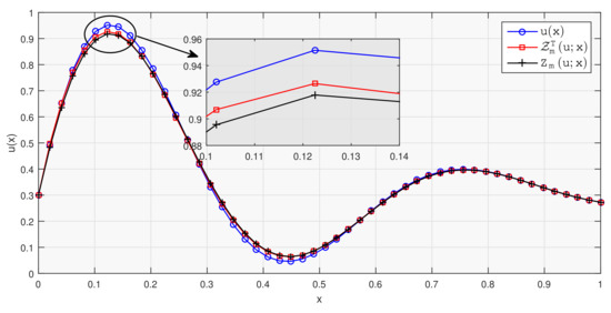
Figure 1. Test function (Blue-Circle), standard Meyer–König and Zeller operator (Black-Plus), and new construction of Meyer–König and Zeller operator (Red-Square) with the given parameters, $r_m\left(x\right)$, $s_m\left(x\right)$, and $\tau \left(x\right)$ on uniform grid.

6.2. Experiment 2

In the second experiment, we take the test function by

$$u\left(x\right)=x^{1/4}sin\left(9x\right),x\in [0,1].$$

and the parameters of the operator by

$$r_m\left(x\right)={\displaystyle \frac{x}{m^{88}}},s_m\left(x\right)={\displaystyle \frac{x}{m^{84}}},\mathrm{and}\tau \left(x\right)=x,$$

on equally spaced 50 grid points on $[0,1]$.

In this experiment, we presented some numerical results of newly define Meyer–König and Zeller operators with different values of m, say $25,50,75,100$. All these results plotted at the same figure labelled Figure 2. According to this figure, with the increase in m, the newly defined operator converged better to the test function, which can be shown in Figure 2.

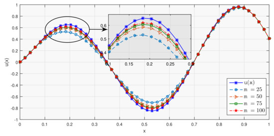
Figure 2. Test function (Blue-Star) and new construction of Meyer–König and Zeller operator with the given parameters, ${\alpha }_n\left(x\right)$, ${\beta }_n\left(x\right)$, and $\rho \left(x\right)$ on uniform grid; $m=25$ (Marine-Hexagram), $m=50$ (Orange-Right Pointing Triangle), $m=75$ (Green-Square), $m=100$ (Red-Star).

All these experiments demonstrate that the newly introduced operators perform well with the properly selected parameters $r_m\left(x\right)$, $s_m\left(x\right)$, and $\tau \left(x\right)$.

7. Concluding Remarks

In this paper, we introduced a generalization of Meyer–König and Zeller operators which depends on a function $\tau \left(x\right)$ by using two sequences of functions, $r_m\left(x\right)$ and $s_m\left(x\right)$. By properly selected $r_m\left(x\right)$, $s_m\left(x\right)$, and $\tau \left(x\right)$, the existing Meyer–König and Zeller operators can be readily produced via introduced operators. In order that the new operator is an approximation procedure, we provide Voronovskaya type theorem, quantitative results and local approximation properties. At the end, we present a couple of numerical examples by using Matlab for different functions. As a future work, the newly introduced Meyer–König and Zeller operators can be applied to numerical solution of integral equations.

References

- Weierstrass, K. Über die analytische Darstellbarkeit sogenannter willkürlicher funktionen einer reellen Veranderlichen. Sitzungsberichte der Akademie zu Berlin 1885, 2, 633–639. [Google Scholar]
- Bernstein, S. Demonstration du theoreme de Weierstrass, fondee sur le calculus des piobabilitts. Commun. Soc. Math. Kharkow. 1913, 13, 1–2. [Google Scholar]
- Usta, F. Approximation of functions by new classes of linear positive operators which fix {1,φ} and {1,φ2}. An. Ştiint. Univ. ‘Ovidius’ Constanta Ser. Mat. 2020, 28, 255–265. [Google Scholar]
- Müller, M.W. Die Folge der Gamma operatoren. Ph.D. Thesis, University Stuttgart, Stuttgart, Germany, 1967. [Google Scholar]
- Sikkema, P.C. On some linear positive operators. Indag. Math. 1970, 32, 327–337. [Google Scholar] [CrossRef]
- Lupaş, A.; Müller, M.W. Approximation properties of the Mn-operators. Aequationes Math. 1970, 5, 19–37. [Google Scholar] [CrossRef]
- Becker, M.; Nessel, R.J. A global approximation theorem for Meyer-König and Zeller operators. Math. Z. 1978, 160, 195–206. [Google Scholar] [CrossRef]
- Alkemade, J.A.H. The second moment for the Meyer-König and Zeller operators. J. Approx. Theory 1984, 40, 261–273. [Google Scholar] [CrossRef][Green Version]
- Abel, U. The moments for the Meyer-König and Zeller operators. J. Approx. Theory 1995, 82, 352–361. [Google Scholar] [CrossRef]
- Braha, N.L.; Mansour, T.; Mursaleen, M. Approximation by Modified Meyer–König and Zeller Operators via Power Series Summability Method. Bull. Malays. Math. Sci. Soc. 2021, 44, 2005–2019. [Google Scholar] [CrossRef]
- Kadak, U.; Khan, A.; Mursaleen, M. Approximation by Meyer König and Zeller operators using (p,q)-calculus. arXiv 2016, arXiv:1603.08539v2. [Google Scholar]
- Cardenas-Morales, D.; Garrancho, P.; Raşa, I. Bernstein-type operators which preserve polynomials. Comput. Math. Appl. 2011, 62, 158–163. [Google Scholar] [CrossRef]
- Erençin, A.; Raşa, I. Voronovskaya type theorems in weighted spaces. Numer. Funct. Anal. Optim. 2016, 37, 1517–1528. [Google Scholar] [CrossRef]
- Acar, T.; Aral, A.; Raşa, I. Modified Bernstein-Durrmeyer operators. Gen. Math. 2014, 22, 27–41. [Google Scholar]
- Aral, A.; Inoan, D.; Raşa, I. On the generalized Szász–Mirakyan operators. Results Math. 2014, 65, 441–452. [Google Scholar] [CrossRef]
- Aral, A.; Ulusoy, G.; Deniz, E. A new construction of Szász-Mirakyan operators. Numer. Algorithms 2018, 77, 313–326. [Google Scholar] [CrossRef]
- Qasim, M.; Khan, A.; Abbas, Z.; Qing-Bo, C. A new construction of Lupaş operators and its approximation properties. Adv. Differ. Equ. 2021, 2021, 51. [Google Scholar] [CrossRef]
- Usta, F. Approximation of functions by a new construction of Bernstein-Chlodowsky operators: Theory and applications. Numer. Methods Partial Differ. Equ. 2021, 37, 782–795. [Google Scholar] [CrossRef]
- Usta, F. On Approximation Properties of a New Construction of Baskakov Operators. Adv. Differ. Equ. 2021, 2021, 269. [Google Scholar] [CrossRef]
- Usta, F. A new approach on the construction of Balázs Type operators. Math. Slovaca 2021. accepted. [Google Scholar]
- Taş, E.; Yurdakadım, T. Variational approximation for modified Meyer-König and Zeller operators. Sarajevo J. Math. 2014, 10, 93–102. [Google Scholar]
- Meyer-König, W.; Zeller, K. Bernsteinsche potenzreihen. Studia Math. 1960, 19, 89–94. [Google Scholar] [CrossRef]
- Rempulska, L.; Skorupka, M. Approximation by generalized MKZ-operators in polynomial weighted spaces. Anal. Theory Appl. 2007, 23, 64–75. [Google Scholar] [CrossRef]
- Erençin, A.; Başcanbaz-Tunca, G.; Taşdelen, F. Some preservation properties of MKZ-Stancu type operators. Sarajevo J. Math. 2019, 15, 113–127. [Google Scholar] [CrossRef]
- Doğru, O.; Örkçü, M. King type modification of Meyer-König and Zeller operators based on the q-integers. Math. Comp. Model. 2009, 50, 1245–1251. [Google Scholar] [CrossRef]
- Shisha, O.; Mond, B. The degree of convergence of sequences of linear positive operators. Proc. Natl. Acad. Sci. USA 1968, 60, 1196–1200. [Google Scholar] [CrossRef]
- Freud, G. On approximation by positive linear methods I, II. Stud. Sci. Math. Hung. 1967, 2, 63–66, Erratum in 1968, 3, 365–370. [Google Scholar]
- Paltanea, R. Optimal estimates with modulus of continuity. Results Math. 1997, 32, 318–331. [Google Scholar] [CrossRef]
- Peetre, J. A Theory of Interpolation of Normed Spaces; Notas de Matemática 39; Instituto de Matemática Pura e Aplicada: Rio de Janeiro, Brazil, 1963; Volume 39. [Google Scholar]
Publisher’s Note: MDPI stays neutral with regard to jurisdictional claims in published maps and institutional affiliations. |
© 2021 by the authors. Licensee MDPI, Basel, Switzerland. This article is an open access article distributed under the terms and conditions of the Creative Commons Attribution (CC BY) license (https://creativecommons.org/licenses/by/4.0/).