Analysis and Synchronization of a New Hyperchaotic System with Exponential Term

Abstract

In this paper, a new four-dimensional hyperchaotic system with an exponential term is presented. The basic dynamical properties and chaotic behavior of the new attractor are analyzed. It can be shown that this system possesses either a line of equilibria or a single one. The existence of hyperchaos is confirmed by its Lyapunov exponents. Moreover, the synchronization problem for the hyperchaotic system is studied. Based on the Lyapunov stability theory, an adaptive control law with two inputs is proposed to achieve the global synchronization. Numerical simulations are given to validate the correctness of the proposed control law.

1. Introduction

It is well known that Lorenz found the first three-dimensional chaotic system, which is named the Lorenz system, when he studied atmospheric convection [1,2]. Since then, many other three-dimensional chaotic systems, i.e., neighboring systems of the Lorenz system, were introduced. For example, Chen [3] constructed a three-dimensional chaotic system, which is similar to the Lorenz system while they are not topologically equivalent. After that, the Lü system [4] was found, and Lü et al. [5] proposed a three-dimensional unified chaotic system that could represent the three different chaotic systems as its special cases. Moreover, hyperchaos, which was first proposed by Rössler [6], has attracted increasing attention from scientific and engineering communities. For instance, based on the Chua’s circuit, Chua et al. [7] realized the hyperchaotic circuit implementation for the first time. Kapitaniak et al. [8] obtained two new hyperchaotic systems through a chain of coupled Chua’s circuits. Wang [9] constructed a four-dimension hyperchaotic Lorenz system by introducing a nonlinear control term to the Lorenz system. Liu et al. [10] proposed a hyperchaotic Liu system that has only one equilibrium point. Abdul et al. [11] proposed a new four-dimentional hyperchaotic system that produces different multistable regions when a trigonometric function was added into a single variable.

To discern chaos and hyperchaos, the positive Lyapunov exponent of a dynamical system is extremely important. A variety of chaotic systems, such as the Liu system, the Lü system and others show a strange attractor with a positive Lyapunov exponent, extending in one direction. In comparison, Hyperchaos characterizes a strange attractor with more than one positive Lyapunov exponent, extending in at least two different directions and exhibiting more complex dynamic behaviors. Hyperchaos can also be used in areas that are wider than chaos.

Many scientists have been interested in chaotic and hyperchaotic systems over recent decades with a large number of equilibrium points, such as systems that have a circular equilibrium [12], systems that have a square equilibrium [13], and systems that have a line equilibrium [14]. It is interesting that Zhou and Yang have found a four-dimensional system with an uncountable number of equilibrium points on a line [15], which is similar to the hyperchaotic system that is proposed in this paper. Zhang and Wang proposed a multiscroll hyperchaotic system with hidden attractors which has infinite number of equilibria [16]. They studied the dynamics properties and the adaptive synchronization of this system. Hyperchaotic systems with infinite equilibrium points and their implementations need to be further studied.

The synchronization of chaotic systems has been also intensively investigated since the pioneer work of Pecora and Carroll [17] in 1990, due to its possible applications in secure communication [18,19], biomedical engineering [20], information science [21] and so on. Many classic control methods and techniques have been applied to the synchronization of the hyperchaotic systems, such as observer design [22,23], the linear feedback control [24,25], the adaptive control [26,27,28,29] the backstepping control [30,31], etc.

So far, there are a few chaotic and hyperchaotic systems with an exponential term such as Ten-ring chaotic system and others [32,33,34,35,36]. Based on the popular Lorenz hyperchaotic system [37], in this paper we propose a new four-dimensional hyperchaotic system with an exponential term and investigate its basic dynamics and properties. More specifically, some complex dynamics will be studied in depth by the Lyapunov exponent continuum, bifurcation diagrams, Poincaré maps and the frequency spectral analysis. Moreover, the synchronization problem for this new hyperchaotic system is studied as well. An adaptive control law with two inputs is proposed and proved by using the Lyapunov stability theory, the Lipschitz saturation extension and the mean value theorem.

The paper is organized as follows. In Section 2, a new four-dimensional hyperchaotic system is established and its basic dynamical properties are analyzed. Section 3 studies the dynamics behaviors for varying parameters. Based on the Lyapunov stability theory, in Section 4 the synchronization problem for the new hyperchaotic system is studied and an adaptive control law is derived and proved. Our conclusions are given in Section 5.

2. A New Hyperchaotic System and Its Dynamical Properties

In this paper, we propose a new hyperchaotic system which contains an exponential term and is described by

$$\left\{\begin{array}{c}{\dot{x}}_1=a(x_2-x_1)+x_4,\hfill \\ {\dot{x}}_2=b{x}_1+x_2-x_1{x}_3,\hfill \\ {\dot{x}}_3=-c{x}_3+e^{x_1{x}_2},\hfill \\ {\dot{x}}_4=d{x}_2{x}_3,\hfill \end{array}\right.$$

(1)

where $(x_1,x_2,x_3,x_4)\in \Omega \subset {\mathbb{R}}^4$, is the state and $a,b,c,d$ are constant parameters. Obviously, the solution of system (1) exists.

2.1. Equilibrium Points

The equilibrium points can be obtained by solving ${\dot{x}}_1={\dot{x}}_2={\dot{x}}_3={\dot{x}}_4=0$, that is

$$\left\{\begin{array}{c}a(x_2-x_1)+x_4=0,\hfill \\ b{x}_1+x_2-x_1{x}_3=0,\hfill \\ -c{x}_3+e^{x_1{x}_2}=0,\hfill \\ d{x}_2{x}_3=0.\hfill \end{array}\right.$$

(2)

It can be easily shown that if $b=1/c$, then system (1) has a line of equilibrium points $E^{*}=(x^{*},0,1/c,a{x}^{*})$. Otherwise, there exists only a single equilibrium point $E_0=(0,0,1/c,0)$.

Linearizing system (1) at the equilibrium $(x_1,x_2,x_3,x_4)$, we can obtain the Jacobian matrix as follows

$$J=\left[\begin{array}{cccc}-a& a& 0& 1\\ b-x_3& 1& -x_1& 0\\ x_2{e}^{x_1{x}_2}& x_1{e}^{x_1{x}_2}& -c& 0\\ 0& d{x}_3& d{x}_2& 0\end{array}\right].$$

(3)

For the equilibrium $E_0=(0,0,1/c,0)$, the characteristic equation is given by

$$(\lambda +c)({\lambda }^3+(a-1){\lambda }^2+(\frac{a}{c}-ab-a)\lambda +\frac{d}{c^2}-\frac{bd}{c})=0.$$

(4)

According to the Routh–Hurwitz criterion, for

$$\begin{array}{c}c>0,a>1,(a-1)(\frac{a}{c}-ab-a)-\frac{d}{c^2}+\frac{bd}{c}>0,\hfill \end{array}$$

(5)

the equilibrium $E_0$ is locally asymptotically stable.

For the equilibrium $E^{*}=(x^{*},0,1/c,a{x}^{*})$, the characteristic equation is given by

$$\begin{array}{cc}\hfill & \lambda ({\lambda }^3+(a+c-1){\lambda }^2+(x^{*2}-c+a(c-1))\lambda -a(c-x^{*2}))=0.\hfill \end{array}$$

(6)

Obviously, Equation (6) has one zero eigenvalue ${\lambda }_1=0$. Therefore, the equilibrium $E^{*}$ is a non-hyperbolic equilibrium point. Again, according to the Routh–Hurwitz criterion, for

$$\begin{array}{c}a+c>1,2a+2c-ac-x^{*2}-1>0,\hfill \end{array}$$

(7)

the equilibrium $E^{*}$ is locally asymptotically stable.

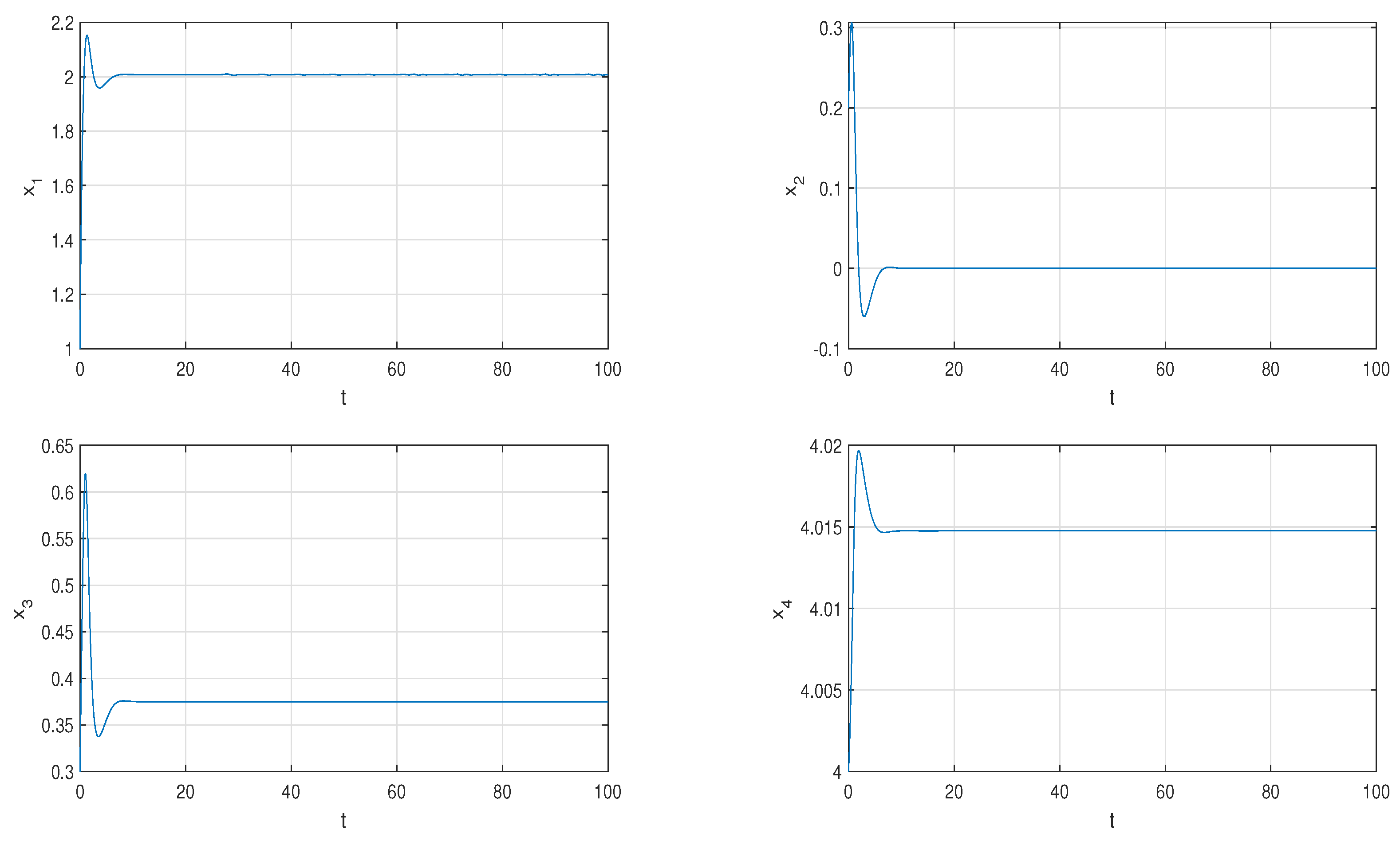
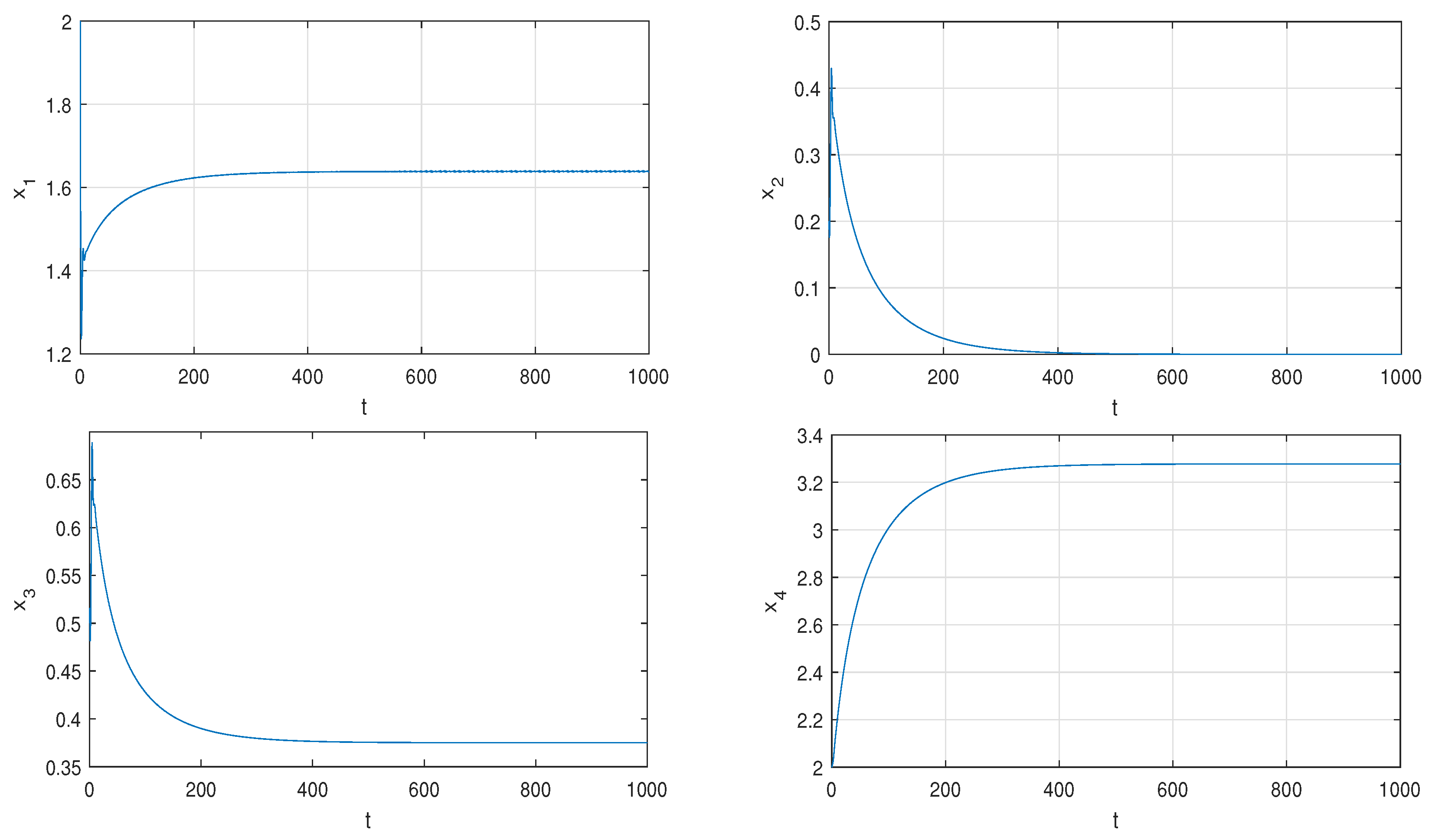
Taking the parameters as $a=2$, $b=\frac{3}{8}$, $c=\frac{8}{3}$, $d=0.1$, we find that for the initial value $(x_1,x_2,x_3,x_4)=(1,0.2,0.3,4)$ system (1) converges to the equilibrium point $E^{*}=(2.0070,0,0.3750,4.0148)$, as shown in Figure 1.

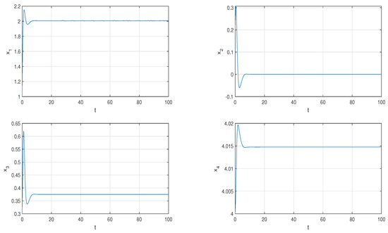
Figure 1. For the initial value $(x_1,x_2,x_3,x_4)=(1,0.2,0.3,4)$ system (1) converges to the equilibrium point $E^{*}=(2.0070,0,0.3750,4.0148)$.

If we change the initial value to $(x_1,x_2,x_3,x_4)=(2,0.2,0.5,2)$, system (1) converges to the equilibrium point $E^{*}=(1.6385,0,0.3750,3.2774)$, as shown in Figure 2.

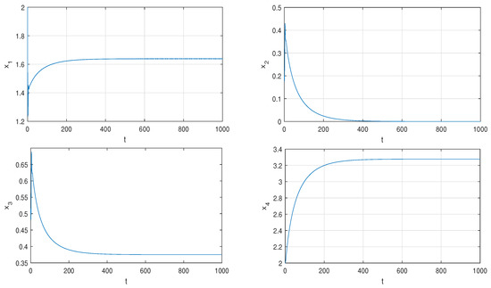
Figure 2. For the initial value $(x_1,x_2,x_3,x_4)=(2,0.2,0.5,2)$ system (1) converges to the equilibrium point $E^{*}=(1.6385,0,0.3750,3.2774)$.

If we choose parameters $a=2$, $b=2$, $c=0.5$, $d=0.1$, system (1) generates periodic solutions as illustrated in Figure 3.

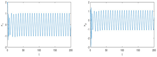
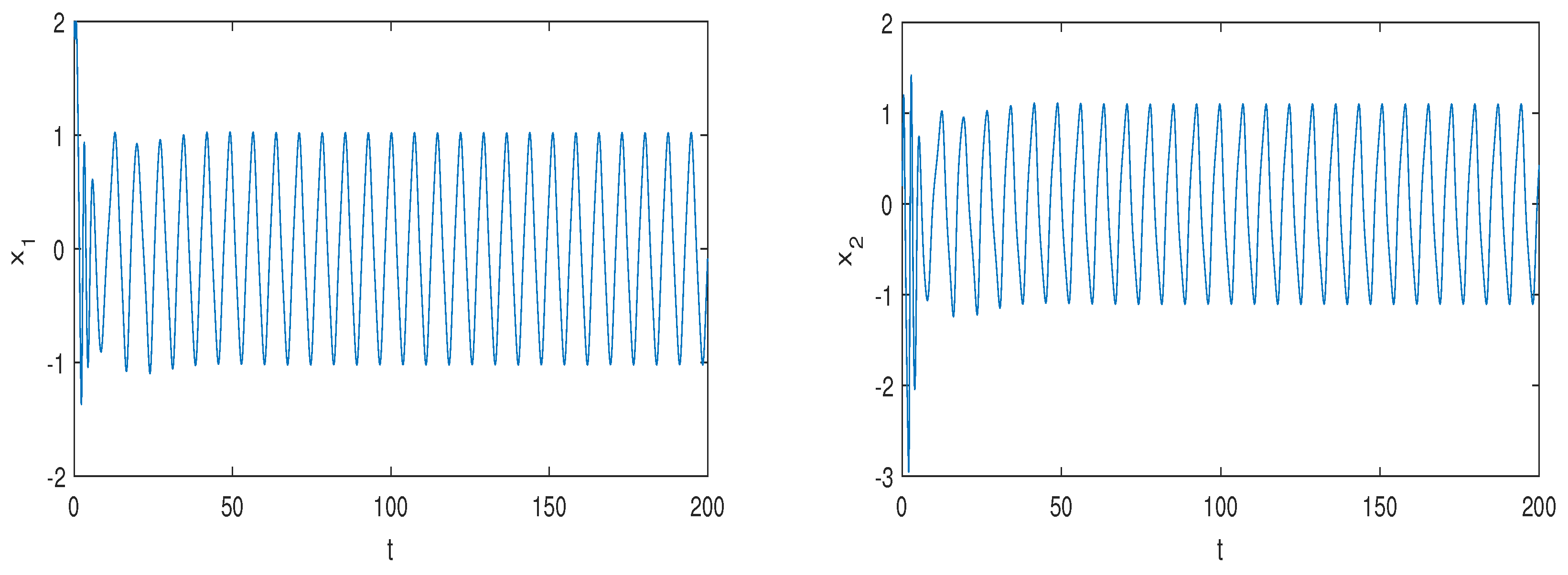
Figure 3. System (1) generates periodic solutions with $a=2$, $b=2$, $c=0.5$, $d=0.1$.

2.2. Dissipativity and Lyapunov Exponents

Notice that for system (1), we have

$$\begin{array}{c}{\displaystyle \nabla V=\frac{\partial {\dot{x}}_1}{\partial x_1}+\frac{\partial {\dot{x}}_2}{\partial x_2}+\frac{\partial {\dot{x}}_3}{\partial x_3}+\frac{\partial {\dot{x}}_4}{\partial w_4}=-a-c+1,}\hfill \end{array}$$

(8)

which implies that this system is dissipative with an exponential contraction if $a+c>1$. Therefore, all system orbits of system (1) will eventually be confined to a specific subset of zero volume. In other words, the asymptotic motion settles onto an attractor.

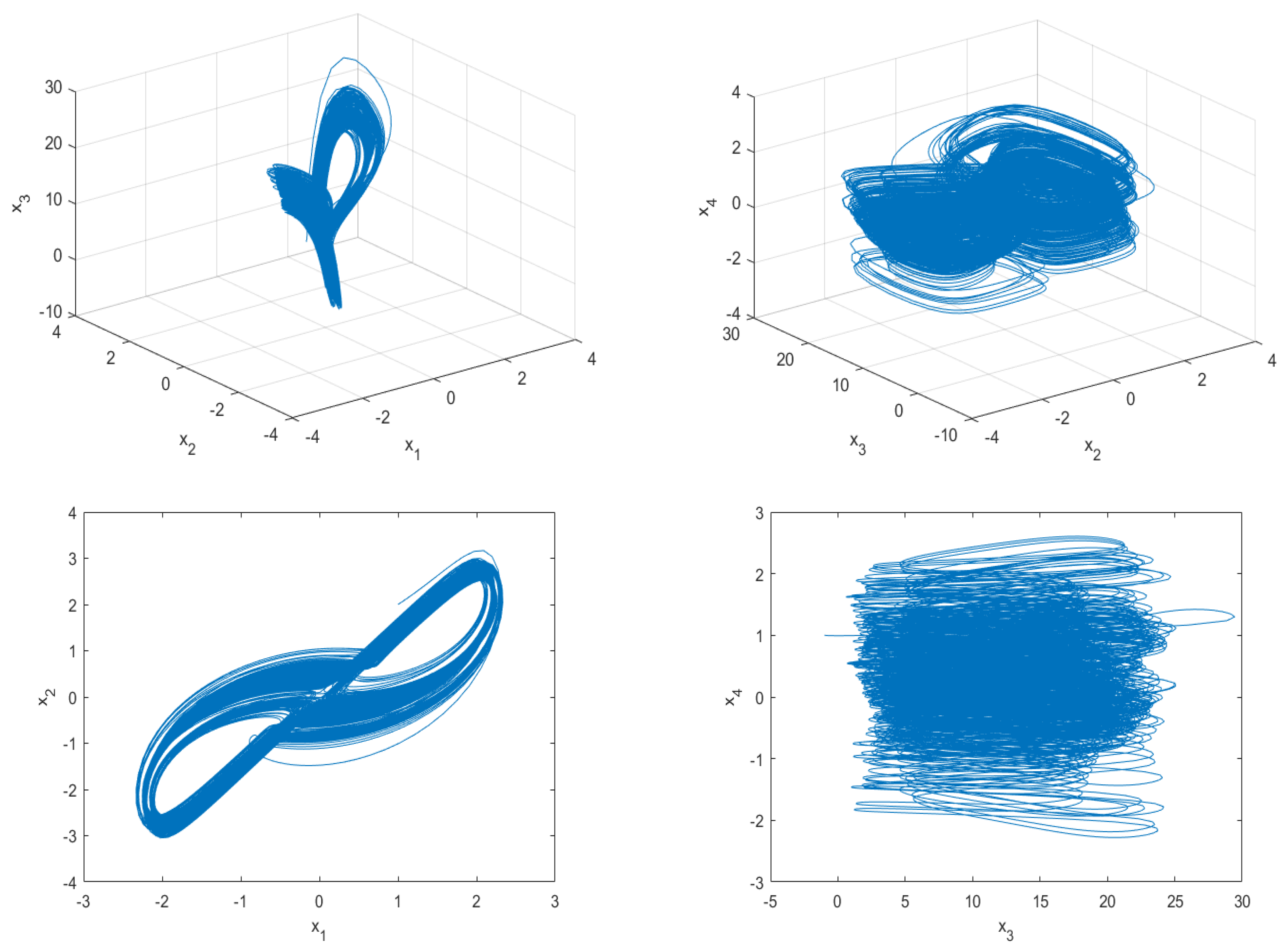
The Lyapunov exponents is a global measure of the rate at which the nearby trajectories diverge and converge in the phase space of system (1). For the parameters $a=10,b=9$, $c=8/3,d=0.1$ and the initial values $x(0)={(0.1,0.1,0.1,0.1)}^{\top }$, the Lyapunov exponents of the system can be obtained as $L_1=0.1782,L_2=0.0217,L_3=0.0000,L_4=-11.8665$. Therefore, system (1) is hyperchaotic since there are two positive Lyapunov exponents. In addition, we can obtain the Kaplan–Yorke fractional dimension as

$${\displaystyle D_L=j+\frac{1}{|L_{j+1}|}\sum _{i=1}^j{L}_i=3.0168.}$$

(9)

For this choice, the strange attractors are shown in Figure 4.

Figure 4. Phase portraits of system (1) with $a=10,b=9,c=8/3,d=0.1$.

3. Observation of New Hyperchaotic Attractors

3.1. Fix $b=28,c=8/3,d=0.1$, and Vary a

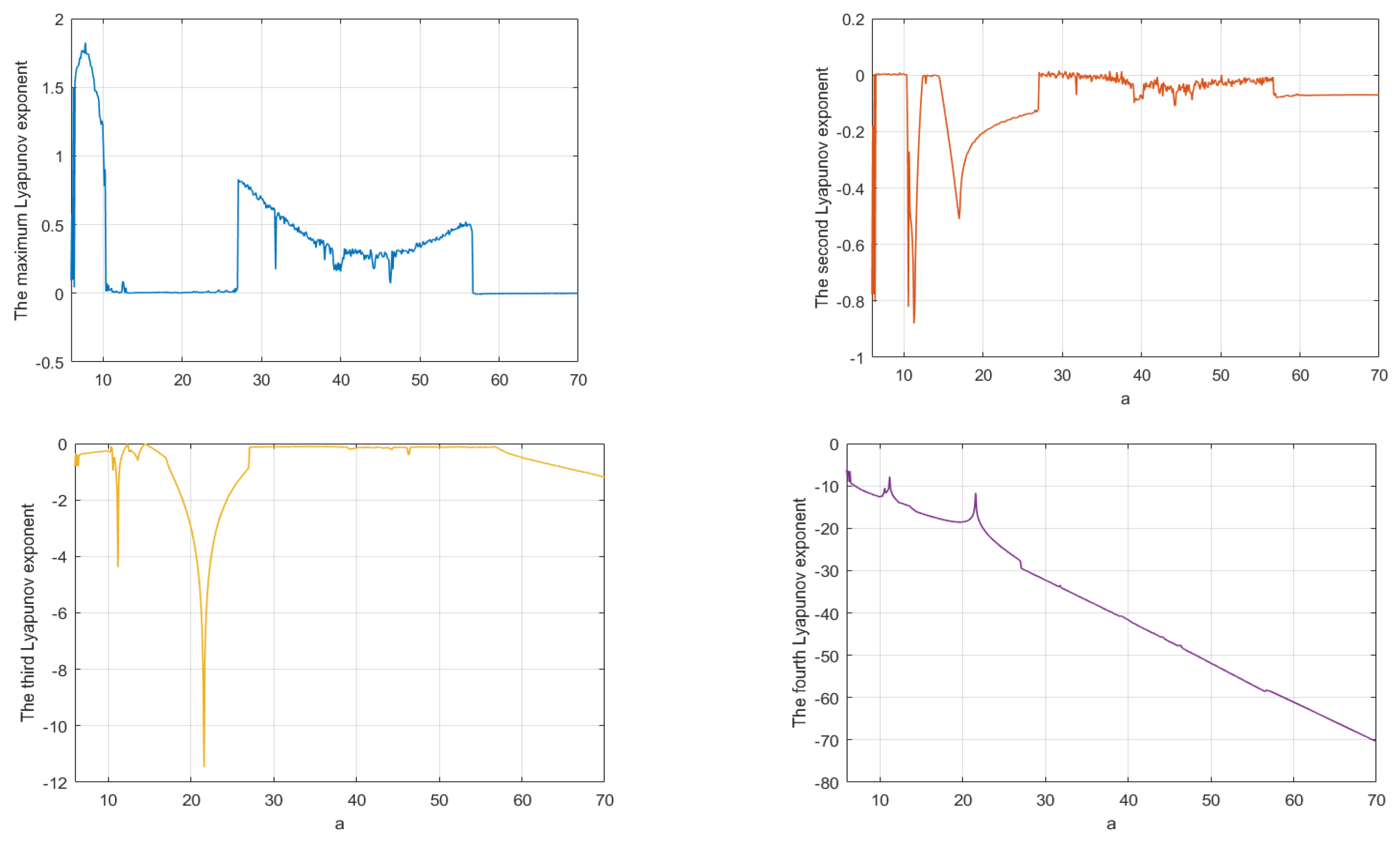
Let parameters $(b,c,d)=(28,8/3,0.1)$ be fixed and parameter a be varied in the interval $[6,70]$. Figure 5 shows the spectrum of Lyapunov exponents of system (1) with respect to the variation of parameter a through MATLAB software in Wolf algorithm.

Figure 5. Spectrum of Lyapunov exponents for $a\in [6,70]$.

For $a\in [6,14)$, there exists one positive Lyapunov exponent, which implies that system (1) is chaotic, and Figure 6a shows the chaotic attractor for $a=6.1$. With a increasing, for $a\in [14,31)$, it can be seen that the maximum Lyapunov exponent is almost equal to zero, which means that the system has a periodic orbit. Figure 6b shows the behavior for $a=20$. Similarly, system (1) is chaotic again for $a\in [31,57)$, as shown in Figure 6c for $a=33$. Furthermore, system (1) is periodic again for $a\in [57,70]$, as shown in Figure 6d for $a=60$. The details are shown in Table 1.

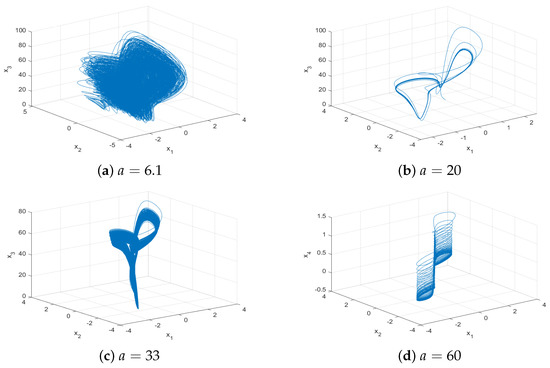
Figure 6. Phase portraits of system (1) for $b=28$, $c=8/3$, $d=0.1$ and different a.

Table 1. The Lyapunov exponents for different a.

a	${\mathit{L}}_1$	${\mathit{L}}_2$	${\mathit{L}}_3$	${\mathit{L}}_4$	Sum of LEs
$6.1$	$1.389229$	$1.70\times {10}^{-5}$	$-0.4569$	$-8.6990$	$-7.7667$
20	$4.6149\times {10}^{-4}$	$-2.030$	$-2.9420$	$-18.5251$	$-21.6667$
33	$0.5048$	$7.6623\times {10}^{-7}$	$-0.1138$	$-35.0577$	$-34.6667$
60	$-5.8093\times {10}^{-9}$	$-0.0735$	$-0.5156$	$-61.0776$	$-61.6667$

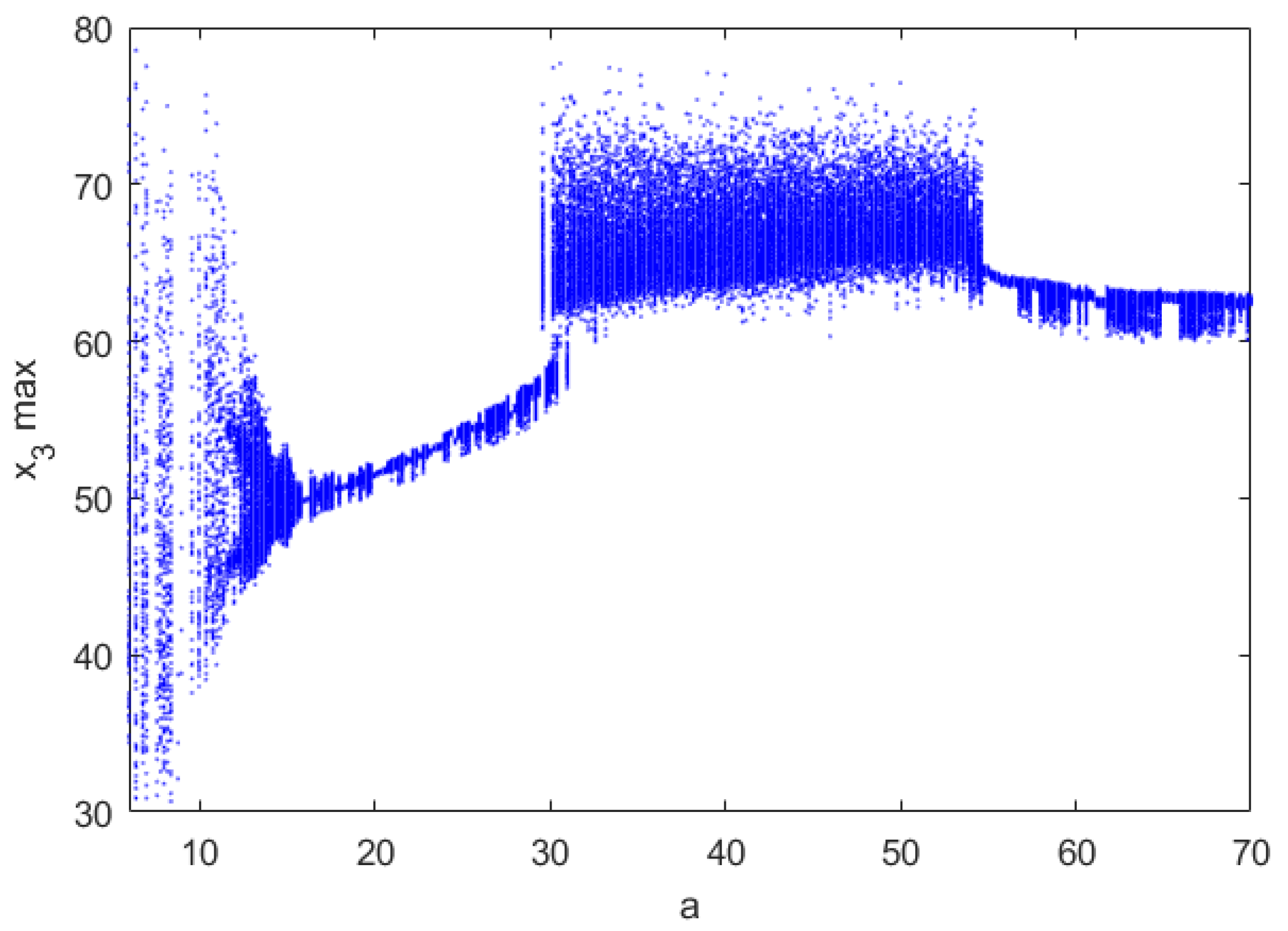
The bifurcation diagram of system (1) with respect to a is shown by Figure 7, which indicates that with a increasing, system (1) switches between chaos and period, and finally degenerates to the periodic solution.

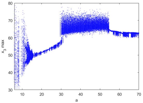
Figure 7. Bifurcation diagram for $a\in [6,70].$

3.2. Fix $a=10,c=8/3,d=0.1,$ and Vary b

Let parameters $(a,c,d)=(10,8/3,0.1)$ be fixed and parameter b be varied in the interval $[0,50]$.

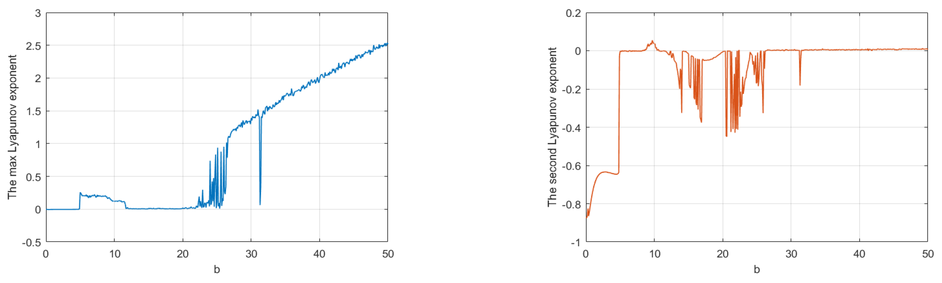
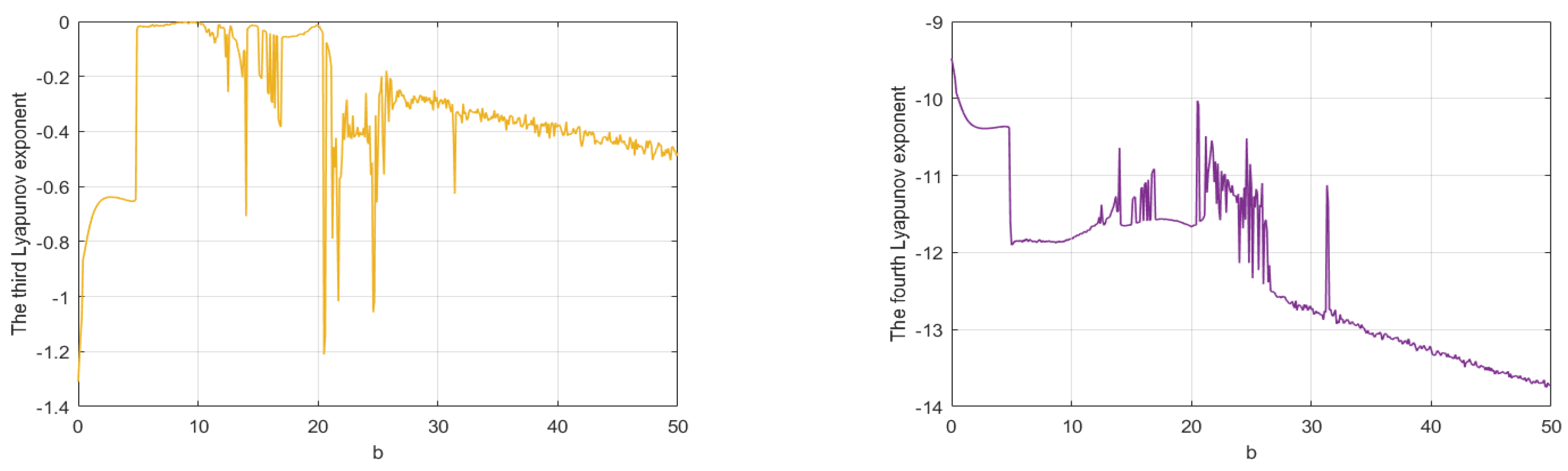
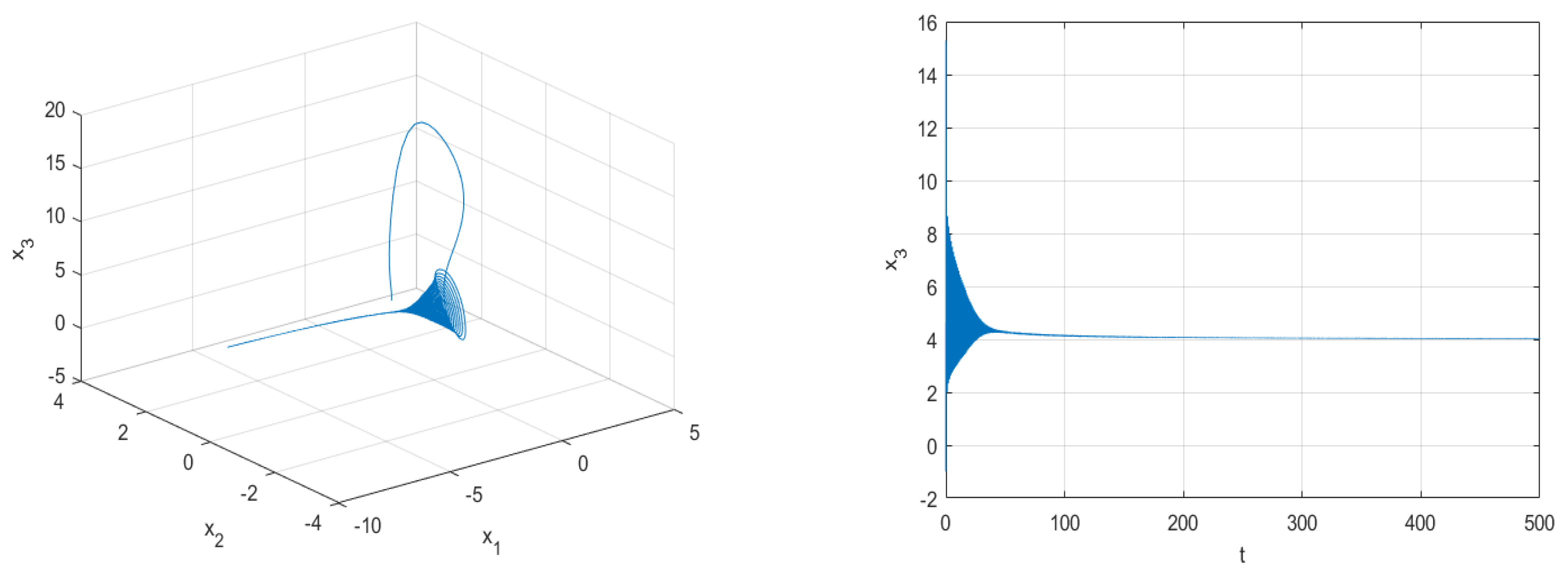
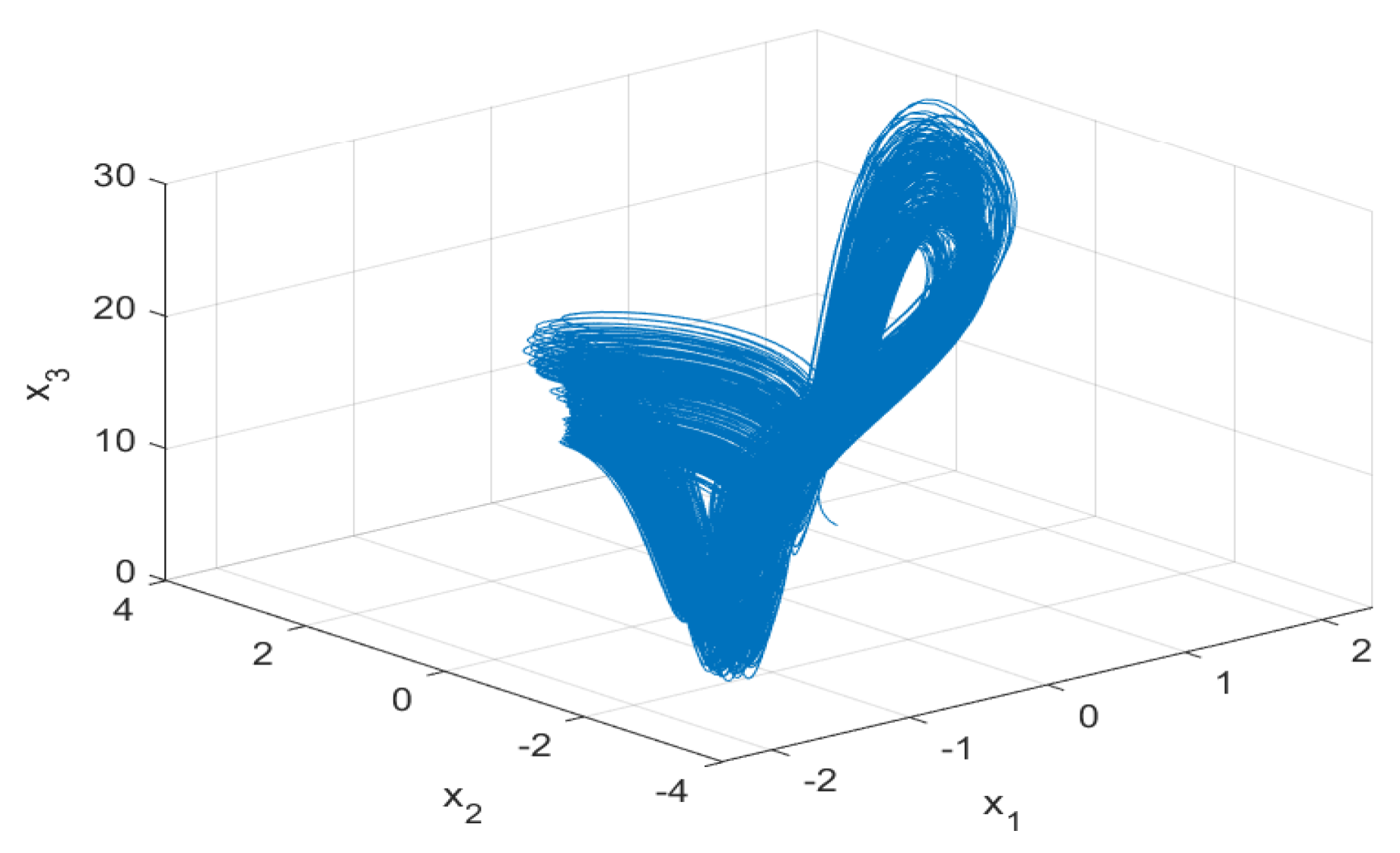
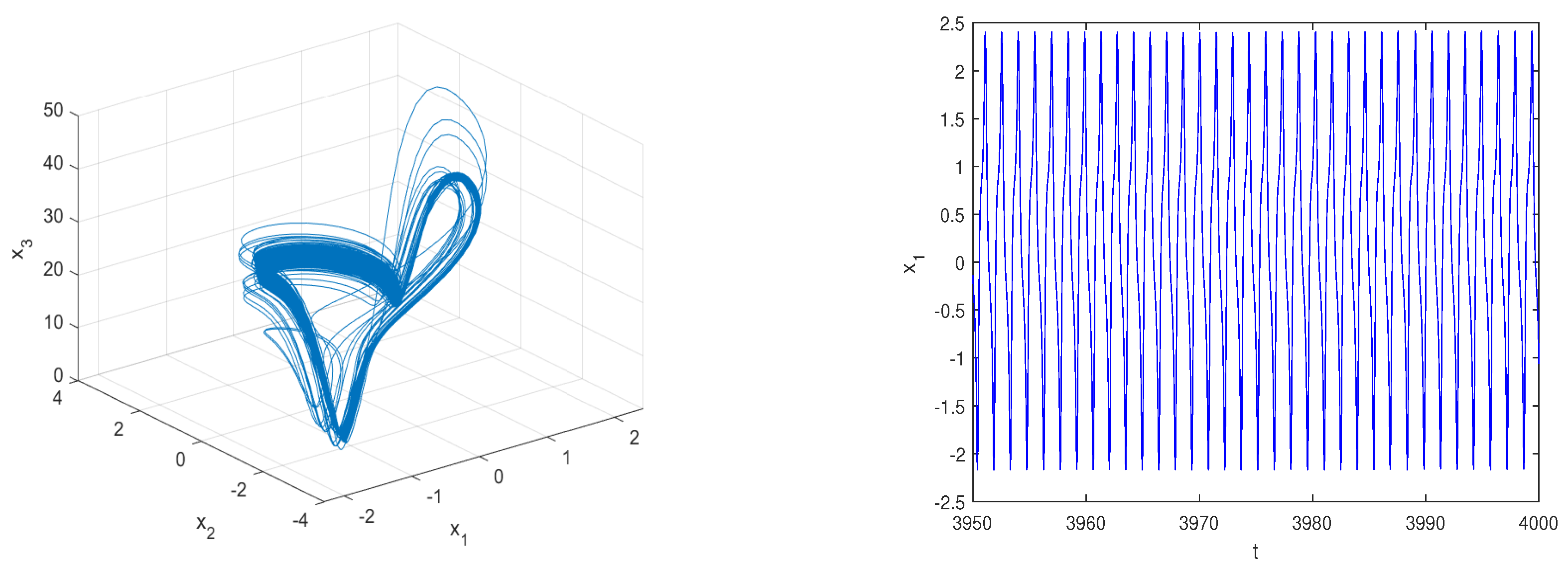
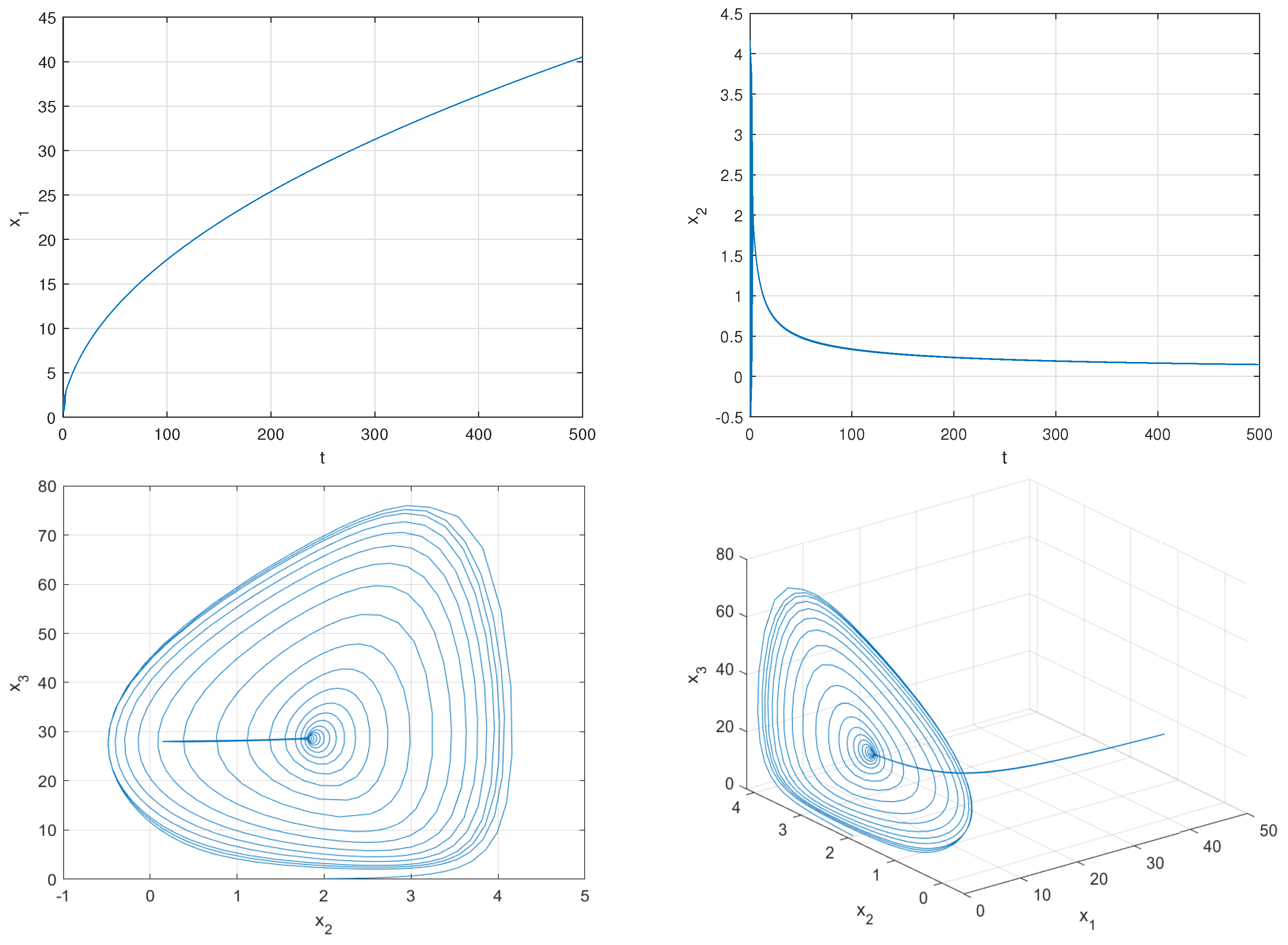
The spectrum of Lyapunov exponents of system (1) with respect to b is shown in Figure 8. It shows that there is none, one or two positive Lyapunov exponents with b in different regions, indicating that system (1) is stable, chaotic or hyperchaotic, respectively. For example, for $b=4$, all the Lyapunov exponents are all negative, and system converges to equilibria (see Figure 9). For $b=10$, there are two positive Lyapunov exponents. In this case, system (1) is hyperchaotic, as shown in Figure 10. For $b=35$, there is one positive Lyapunov exponent, indicating that system (1) is chaotic, as shown in Figure 11. In addition, we also find that the maximum Lyapunov exponent equals to zero for b in some regions, which means that the system has a periodic orbit. Figure 12 shows that system (1) is periodic for $b=14.8$. The details are shown in Table 2.

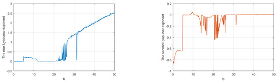
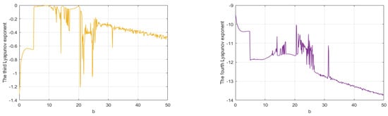
Figure 8. Spectrum of Lyapunov exponents for $b\in [0,50]$.

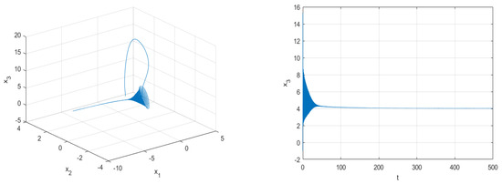
Figure 9. Phase portraits of system (1) for $a=10,c=8/3,d=0.1$, and $b=4$.

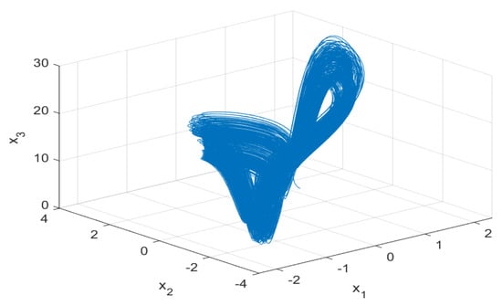
Figure 10. Phase portraits of system (1) for $a=10,c=8/3,d=0.1$ and $b=10$.

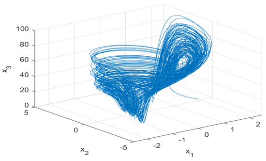
Figure 11. Phase portraits of system (1) for $a=10,c=8/3,d=0.1$, and $b=35$.

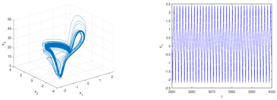
Figure 12. System (1) is periodic for $a=10,c=8/3,d=0.1$, and $b=14.8$.

Table 2. The Lyapunov exponents for different b.

b	${\mathit{L}}_1$	${\mathit{L}}_2$	${\mathit{L}}_3$	${\mathit{L}}_4$	Sum of LEs
4	$-0.0033$	$-0.6434$	$-0.6494$	$-10.3706$	$-11.6668$
10	$0.1169$	$0.0410$	$-2.7077\times {10}^{-8}$	$-11.8245$	$-11.6667$
$14.8$	$5.0049\times {10}^{-4}$	$-0.0097$	$-0.1183$	$-11.5381$	$-11.6667$
35	$1.6801$	$-2.6005\times {10}^{-8}$	$-0.3513$	$-12.9955$	$-11.6667$

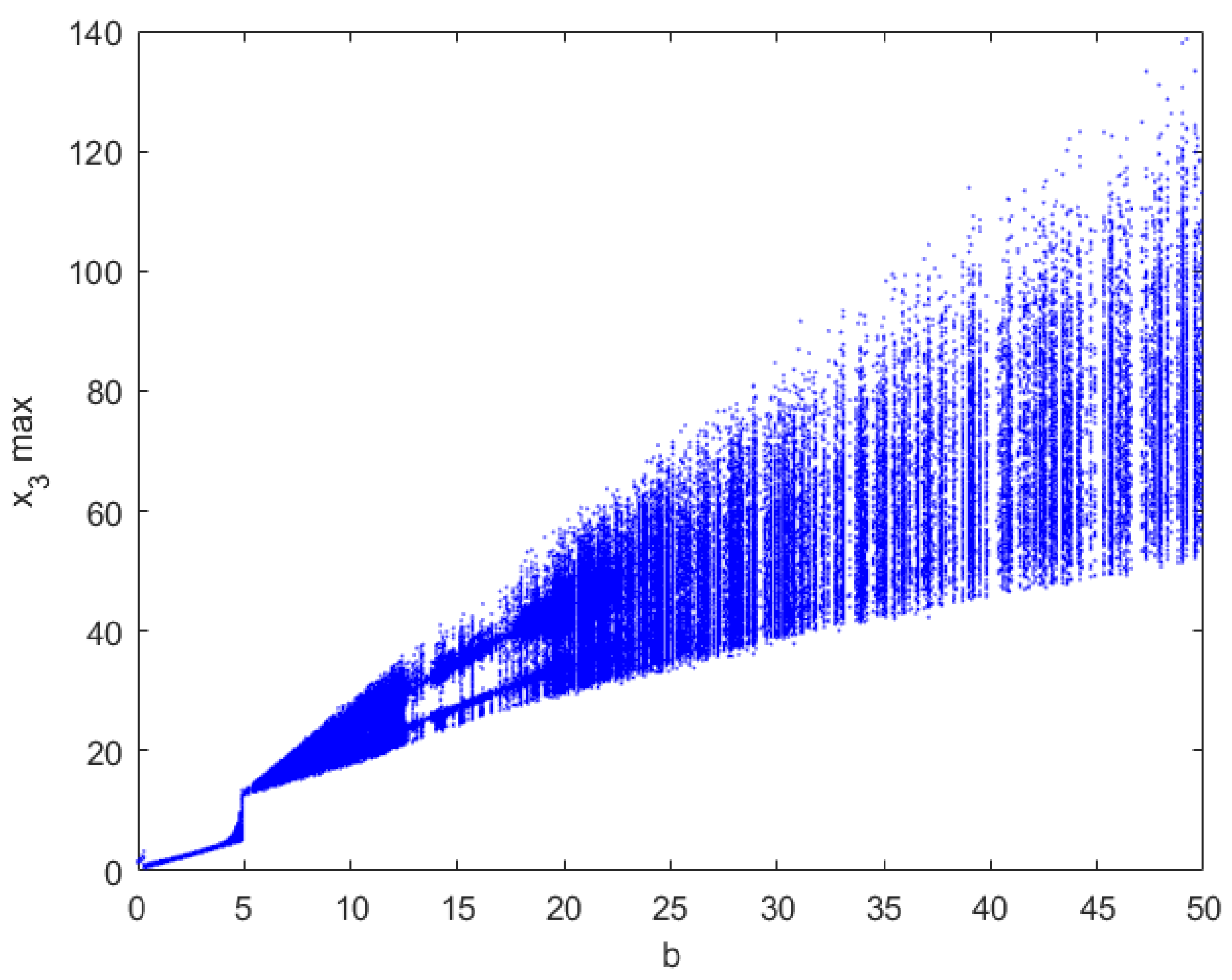
The bifurcation diagram of the system (1) with respect to b is shown in Figure 13, indicating that system (1) may be stable, periodic, chaotic or hyperchaotic.

Figure 13. Bifurcation diagram for $b\in [0,50]$.

3.3. Fix $a=10,b=28,d=0.1,$ and Vary c

Let parameters $(a,b,d)=(10,28,0.1)$ be fixed and parameter c be varied in the interval $[0,14]$.

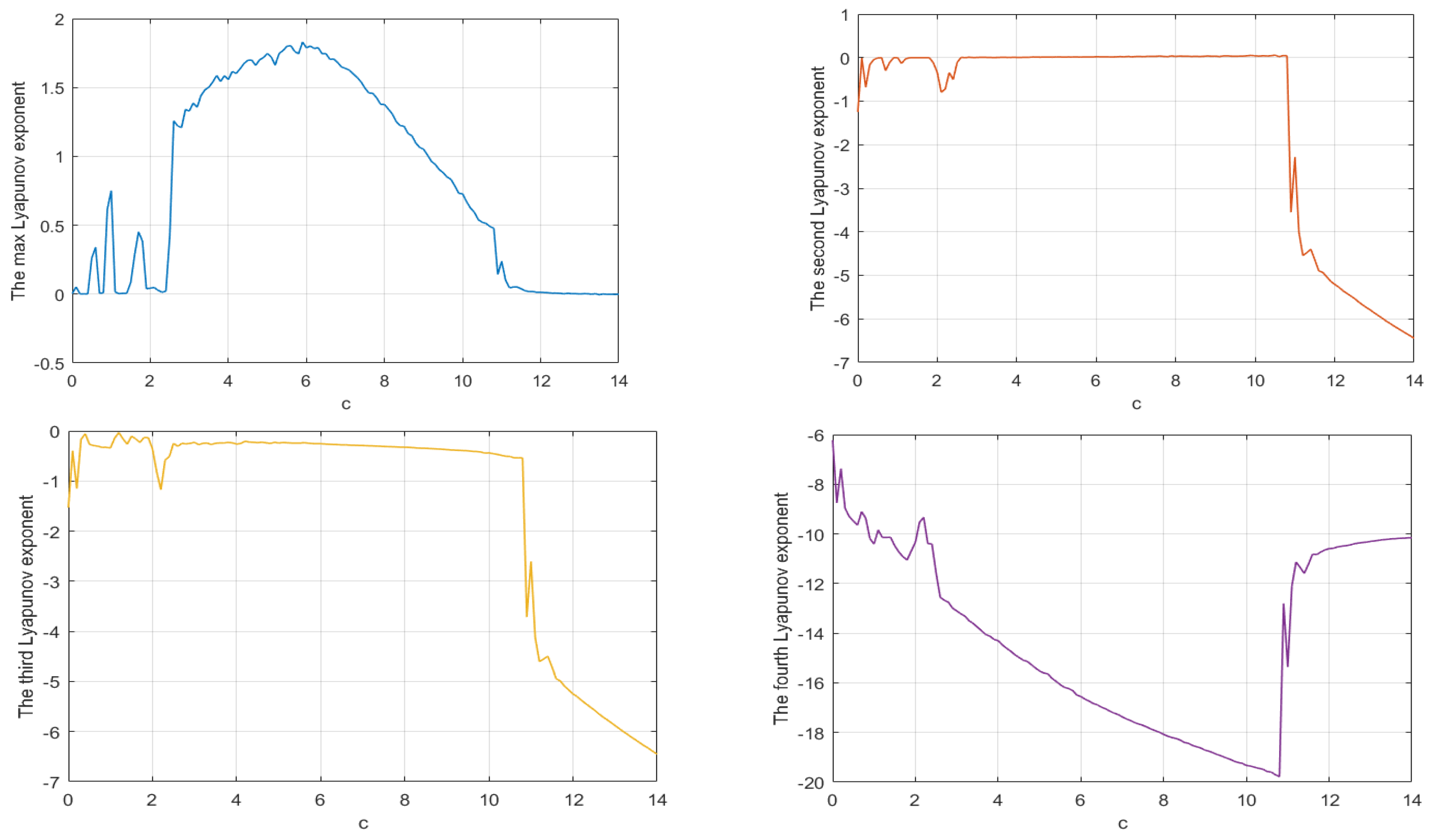
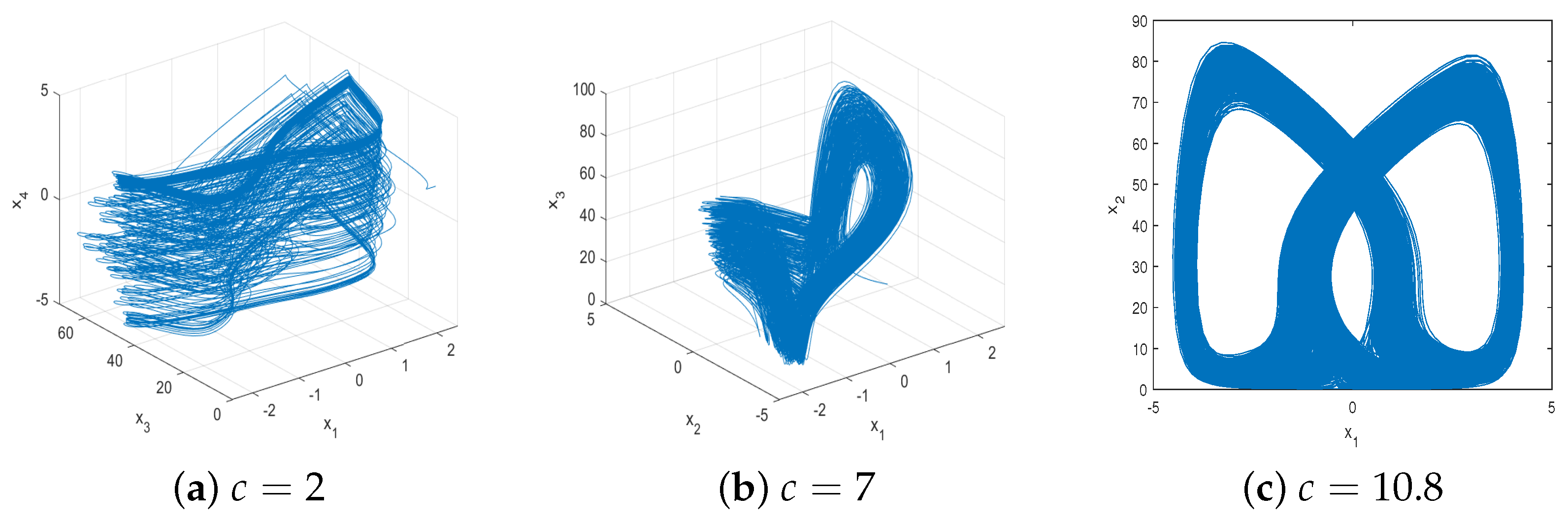
Figure 14 gives the spectrum of Lyapunov exponents of system (1). It shows that system (1) may be chaotic or periodic with different c. For example, for $c=2$, there is only one positive Lyapunov exponent, indicating that system (1) is chaotic, as shown in Figure 15a. Similarly, Figure 15b,c show the chaotic attractor for $c=7$ and $c=10.8$, respectively. However, for $c=14$, it can be seen that the maximum Lyapunov exponent is negative, which means that chaos disappears, as shown in Figure 16. The details are shown in Table 3.

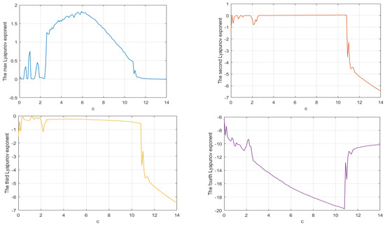
Figure 14. Spectrum of Lyapunov exponents for $c\in [0,14]$.

Figure 15. Phase portraits of system (1) for $a=10,b=28,d=0.1$ and different c.

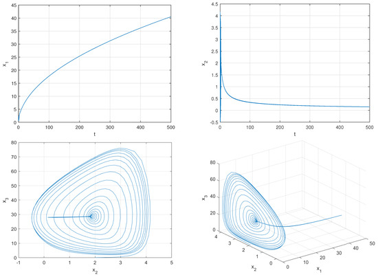
Figure 16. Chaos disappears for $a=10,b=28$ and $d=0.1$ at $c=14$.

Table 3. The Lyapunov exponents for different c.

c	${\mathit{L}}_1$	${\mathit{L}}_2$	${\mathit{L}}_3$	${\mathit{L}}_4$	Sum of LEs
2	$0.4613$	$-5.6506\times {10}^{-5}$	$-0.6869$	$-10.7743$	$-11$
7	$1.6622$	$1.9917\times {10}^{-8}$	$-0.2958$	$-17.3665$	$-16$
$10.8$	$0.6440$	$-3.3697\times {10}^{-7}$	$-0.4877$	$-19.9563$	$-19.8$
14	$-0.0010$	$-5.1933$	$-5.3943$	$-12.4114$	$-23$

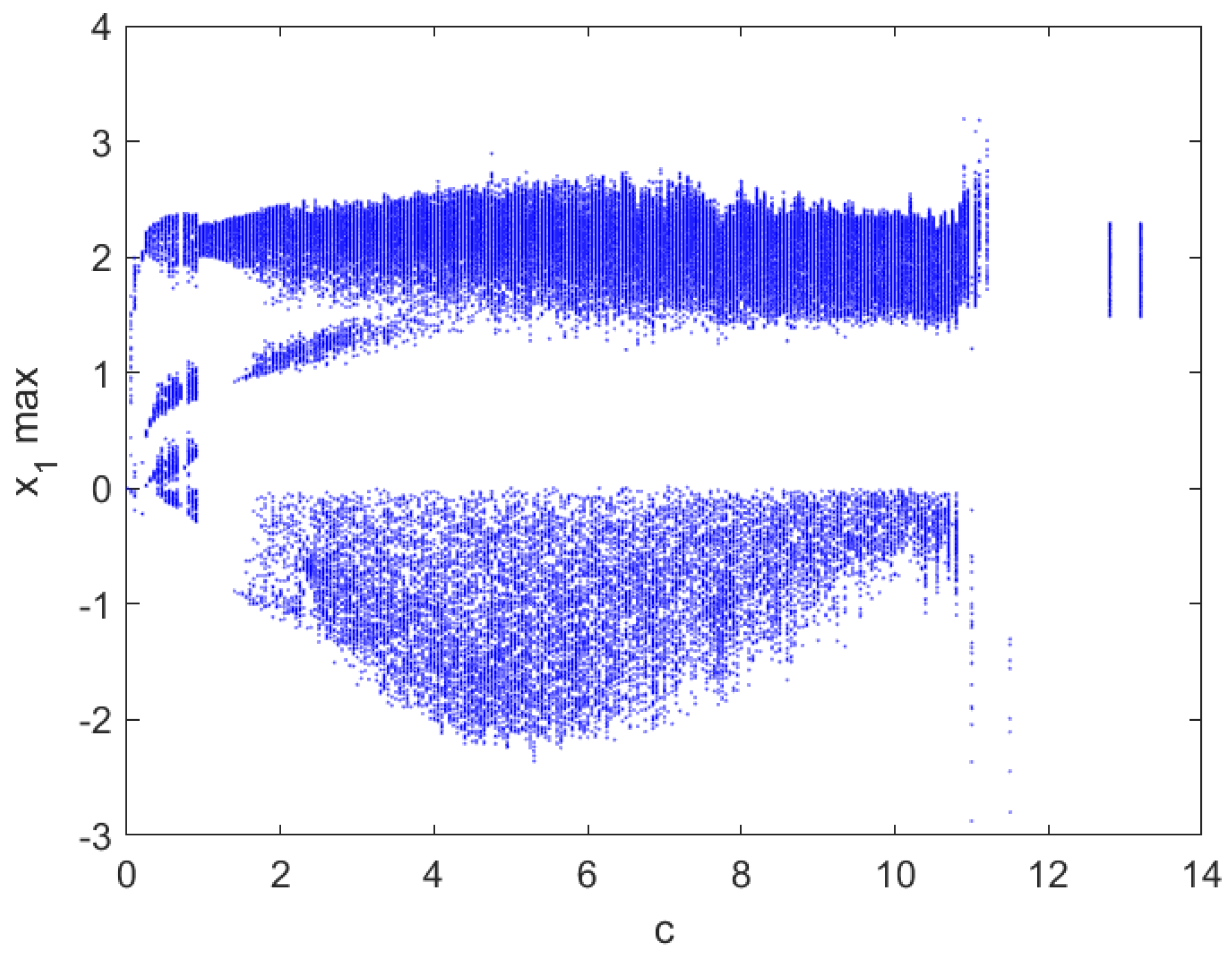
The bifurcation diagram of system (1) with respect to c is shown by Figure 17, which indicates that with c increasing, the new chaotic attractor of system (1) degenerate to the periodic solution.

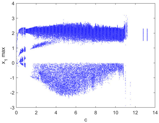
Figure 17. Bifurcation diagram for $c\in [0,14]$.

4. Adaptive Synchronization by Two Inputs

The new hyperchaotic system (1) can be rewritten by

$$\dot{x}=Ax+f(x),$$

(10)

where $x\in \Omega \subset {\mathbb{R}}^4$, $A={(a_{ij})}_{n\times n}$ is a real matrix and $f(x)={(f_1(x),\dots ,f_n(x))}^{\top }$ denotes the nonlinear part of the system which is, obviously, in the following form

$$A=\left[\begin{array}{cccc}-a& a& 0& 1\\ b& 1& 0& 0\\ 0& 0& -c& 0\\ 0& 0& 0& 0\end{array}\right],f(x)=\left[\begin{array}{c}0\\ -x_1{x}_3\\ e^{x_1{x}_2}\\ d{x}_2{x}_3\end{array}\right].$$

In this section, an adaptive control law will be proposed to achieve the synchronization problem for system (10). Let (10) be the master system and construct the following slave system to achieve the synchronization objective

$$\dot{y}=Ay+f(y)+u$$

(11)

where $y={(y_1,y_2,y_3,y_4)}^{\top }$ is the state, $u={(u_1,u_2,u_3,u_4)}^{\top }$ denotes the designed control. Define the error states by $e={(e_1,e_2,e_3,e_4)}^{\top }$, where $e_i=y_i-x_i$, for $1\le i\le 4$. According to the structure of (10) and (11), one obtains the error dynamics

$$\dot{e}=Ae+f(y)-f(x)+u$$

(12)

Since when system (10) exhibits hyperchaotic behavior, $\Omega$ can always be seen as an 4-dimensional bounded closed convex set of ${\mathbb{R}}^4$ and the existence of four positive real constant $M_i$, for $1\le i\le 4$ such that $|x_i|\le M_i$ can be assumed. Since $\Omega$ is bounded, f is locally Lipschitz in $\Omega$. Note that this property can be extended to global Lipschitz by introducing the convectional saturation extension of f (see [38] for the details).

Based on the above analysis and the mean value theorem of two variables, we have

$$\begin{array}{cc}\hfill e^{\top }(f(y)-f(x))=& e_2(-y_1{y}_3+x_1{x}_3)+e_3(e^{y_1{y}_2}-e^{x_1{x}_2})+d{e}_4(y_2{y}_3-x_2{x}_3)\hfill \\ \hfill =& -y_1{e}_2{e}_3-x_3{e}_1{e}_2+(x_2+\theta e_2)e^{(x_1+\theta e_1)(x_2+\theta e_2)}{e}_1{e}_3\hfill \\ \hfill & -(x_1+\theta e_1)e^{(x_1+\theta e_1)(x_2+\theta e_2)}{e}_2{e}_3+d{y}_2{e}_3{e}_4+d{x}_3{e}_2{e}_4\hfill \end{array}$$

(13)

where $0<\theta <1$. According to the saturation extension of f and the convexity property of $\Omega$, we obtain

$$\begin{array}{cc}\hfill e^{\top }(f(y)-f(x))\le & M_1|e_2{e}_3|+M_3|e_1{e}_2|+M_2{e}^{M_1{M}_2}|e_1{e}_3|+M_1{e}^{M_1{M}_2}\left|e_2{e}_3\right|\hfill \\ & +d{M}_2|e_3{e}_4|+d{M}_3\left|e_2{e}_4\right|.\hfill \end{array}$$

Theorem 1.

The master system (10) and the slave system (11) can be globally synchronized by the control scheme

$$u_1=0,u_2=k{e}_2,u_3=0,u_4=k{e}_4,$$

(14)

where k denotes the feedback gain which is updated by the following adaptive law $\dot{k}=-\delta (e_2^2+e_4^2),$ with δ being any arbitrary positive constant.

Proof. 

Choose the following Lyapunov function

$$V=\rho e_1^2+e_2^2+e_3^2+e_4^2+{\delta }^{-1}{(k+L)}^2,$$

where L and $\rho$ are positive constants, which will be determined later. Differentiating V with respect to time t, we obtain

$$\begin{array}{cc}\hfill \dot{V}=& 2[\rho e_1{\dot{e}}_1+e_2{\dot{e}}_2+e_3{\dot{e}}_3+e_4{\dot{e}}_4+{\delta }^{-1}(k+L)\dot{k}]\hfill \\ \hfill =& 2[\rho a{e}_1(e_2-e_1)+\rho e_1{e}_4+e_2(b{e}_1+e_2-L{e}_2)-c{e}_3^2-L{e}_4^2+e^{\top }(f(y)-f(x))]\hfill \\ \hfill \le & 2[-\rho a{e}_1^2-(L-1)e_2^2-c{e}_3^2-L{e}_4^2+(\rho a+b)e_1{e}_2+\rho e_1{e}_4\hfill \\ \hfill & +M_1|e_2{e}_3|+M_3|e_1{e}_2|+M_2{e}^{M_1{M}_2}|e_1{e}_3|+M_1{e}^{M_1{M}_2}|e_2{e}_3|+d{M}_2\left|e_3{e}_4\right|\hfill \\ & +d{M}_3|e_2{e}_4\left|\right]\hfill \\ \hfill \le & -(\rho a-b-\rho -M_3)|e_1{|}^2-(2L-2-\rho a-b-M_1-(1+d)M_3){\left|e_2\right|}^2\hfill \\ \hfill & -(2c-M_1-d{M}_2)|e_3{|}^2-(2L-\rho -d(M_2+M_3))|e_4{|}^2+2M_1{e}^{M_1{M}_2}\left|e_2{e}_3\right|\hfill \\ & +2M_2{e}^{M_1{M}_2}\left|e_1{e}_3\right|\hfill \\ \hfill =& -{\left|e\right|}^{\top }P\left|e\right|,\hfill \end{array}$$

(15)

where $\left|e\right|=(|e_1|,|e_2|,|e_3|,|e_4{|)}^{\top }$ and P is a symmetric matrix of the form

$$\begin{array}{ccc}P\hfill & =\hfill & \left(\begin{array}{cccc}{\alpha }_1& 0& -M_2{e}^{M_1{M}_2}& 0\\ 0& {\alpha }_2& -M_1{e}^{M_1{M}_2}& 0\\ -M_2{e}^{M_1{M}_2}& -M_1{e}^{M_1{M}_2}& {\alpha }_3& 0\\ 0& 0& 0& {\alpha }_4\end{array}\right)\hfill \end{array}$$

(16)

where ${\alpha }_i$, for $1\le i\le 4$, are given by

$$\begin{array}{c}{\alpha }_1=\rho a-\rho -b-M_3,\hfill \\ {\alpha }_2=2L-2-\rho a-b-M_1-(1+d)M_3,\hfill \\ {\alpha }_3=2c-M_1-d{M}_2,\hfill \\ {\alpha }_4=2L-\rho -d(M_2+M_3).\hfill \end{array}$$

(17)

Clearly, if the symmetric matrix P is positive definite, then $\dot{V}\le 0$. Moreover, it is well known that P is positive definite if and only if ${\Delta }_i>0$, for $1\le i\le 4$, where ${\Delta }_i$ denotes the Leading Principle Minor of order i of P. A straightforward calculation gives

$${\Delta }_1={\alpha }_1,{\Delta }_2={\alpha }_2{\Delta }_1,{\Delta }_3={\alpha }_3{\Delta }_2-e^{2M_1{M}_2}({\alpha }_1{M}_1^2+{\alpha }_2{M}_2^2),{\Delta }_4={\alpha }_4{\Delta }_3.$$

From the condition ${\Delta }_i>0$, for $1\le i\le 4$, and the above equalities, it is easy to obtain

$$\begin{array}{ccc}\hfill \rho & >& {\displaystyle \frac{1}{a-1}(\frac{M_2^2{e}^{2M_1{M}_2}}{2c-M_1-d{M}_2}+M_3+b),}\hfill \\ \hfill L& >& {\displaystyle \max \{\frac{1}{2}(2+\rho a+b+M_1+(1+d)M_3),\frac{1}{2}(\rho +d(M_2+M_3))\}.}\hfill \end{array}$$

Therefore, there always exist positive $\rho$ and L satisfying the above conditions so that $\dot{V}\le 0$, and thus V is positive and decrescent. It follows that the equilibrium point $(e_1=0,$$e_2=0,e_3=0,e_4=0,k=k^{*})$ of system (12) is uniformly stable which implies, from (12), that ${\dot{e}}_1(t),{\dot{e}}_2(t),{\dot{e}}_3(t),{\dot{e}}_4(t)$ are also uniformly stable. Furthermore, it can be concluded from (15) that $e_1(t),e_2(t),e_3(t),e_4(t)$ are quadratically integrable, i.e., $e_1(t),e_2(t),e_3(t),e_4(t)\in L_2$. By using Barbalat’s lemma, for any initial values we have always $e_1(t)\to 0,e_2(t)\to 0,e_3(t)\to 0,e_4(t)\to 0$ ($t\to \infty$) and $k\to k^{*}$ ($t\to \infty$), which imply that the master system (10) and slave system (11) are globally asymptotically synchronized under the control law (14). This completes the proof. □

In the following, numerical simulations by MATLAB will be given to validate the correctness and effectiveness of the proposed controller design.

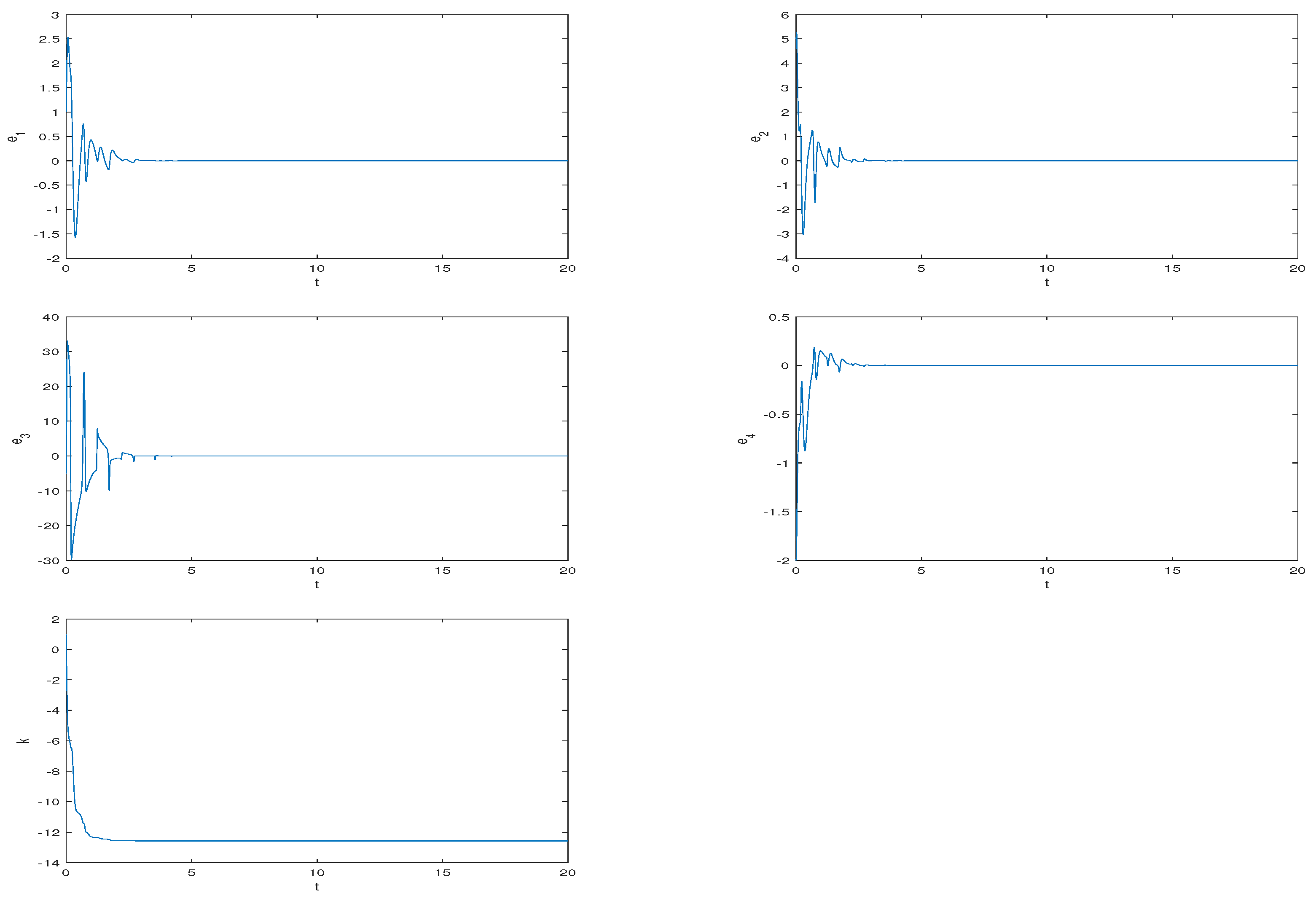
The parameters of system (1) are set to $a=10,b=28,c=8/3,d=0.1$ so that it exhibits hyperchaotic behavior. The initial conditions of the master and slave systems are chosen as $(x_{10},x_{20},x_{30},x_{40})=(1,-2,20,1)$ and $(y_{10},y_{20},y_{30},y_{40})=(2,3,15,-1)$, respectively. Selecting $\delta =4$ and the initial value of k by $k(0)=1$, Figure 18 shows that the error states $e_1(t),e_2(t),e_3(t),e_4(t)$ converge asymptotically to zero while the control gains k tend to a negative constants, as t tends to infinity.

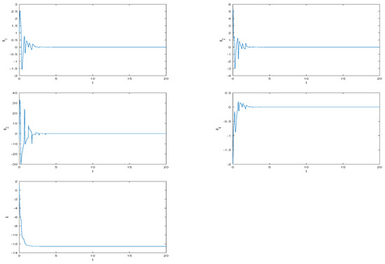
Figure 18. Adaptive synchronization for system (1).

5. Conclusions

Based on the results in [37], we propose a new four-dimensional hyperchaotic system with an exponential term. Comparing with the model in [37], our new four-dimensional hyperchaotic system has an exponential term and it has a line of equilibrium points or a single one. According to the theoretical and simulations, we have given the bifurcation diagram and the Lyapunov exponent spectrum which show that the system may be chaotic or hyperchaotic.

The adaptive synchronization of the proposed hyperchaotic system is also studied and based on the Lyapunov stability theory, an adaptive control law with two inputs is derived to achieve the globally synchronization. Numerical simulations have been done to show the effectiveness of the proposed control law.

References

- Lorenz, E.N. Deterministic nonperiodic flow. J. Atmos. Sci. 1963, 20, 130–141. [Google Scholar] [CrossRef] [Green Version]
- Sparrow, C. The Lorenz Equations: Bifurcations, Chaos, and Strange Attractors; Springer Science & Business Media: Berlin/Heidelberg, Germany, 2012; Volume 41. [Google Scholar]
- Chen, G.; Ueta, T. Yet another chaotic attractor. Int. J. Bifurc. Chaos 1999, 9, 1465–1466. [Google Scholar] [CrossRef]
- Lü, J.; Chen, G. A new chaotic attractor coined. Int. J. Bifurc. Chaos 2002, 12, 659–661. [Google Scholar] [CrossRef]
- Lü, J.; Chen, G.; Cheng, D.; Celikovsky, S. Bridge the gap between the Lorenz system and the Chen system. Int. J. Bifurc. Chaos 2002, 12, 2917–2926. [Google Scholar] [CrossRef]
- Rössler, O. An equation for hyperchaos. Phys. Lett. A 1979, 71, 155–157. [Google Scholar] [CrossRef]
- Chua, L.; Komuro, M.; Matsumoto, T. The double scroll family. IEEE Trans. Circuits Syst. 1986, 33, 1072–1118. [Google Scholar] [CrossRef] [Green Version]
- Kapitaniak, T.; Chua, L.; Zhong, G.Q. Experimental hyperchaos in coupled Chua’s circuits. IEEE Trans. Circuits Syst. I Fundam. Theory Appl. 1994, 41, 499–503. [Google Scholar] [CrossRef]
- Wang, X.; Wang, M. A hyperchaos generated from Lorenz system. Phys. A Stat. Mech. Its Appl. 2008, 387, 3751–3758. [Google Scholar] [CrossRef]
- Liu, L.; Liu, C.; Zhang, Y. Analysis of a novel four-dimensional hyperchaotic system. Chin. J. Phys. 2008, 46, 386. [Google Scholar]
- Rahim, M.A.; Natiq, H.; Fataf, N.; Banerjee, S. Dynamics of a new hyperchaotic system and multistability. Eur. Phys. J. Plus 2019, 134, 1–9. [Google Scholar]
- Gotthans, T.; Petržela, J. New class of chaotic systems with circular equilibrium. Nonlinear Dyn. 2015, 81, 1143–1149. [Google Scholar] [CrossRef] [Green Version]
- Gotthans, T.; Sprott, J.C.; Petrzela, J. Simple chaotic flow with circle and square equilibrium. Int. J. Bifurc. Chaos 2016, 26, 1650137. [Google Scholar] [CrossRef]
- Jafari, S.; Sprott, J. Simple chaotic flows with a line equilibrium. Chaos Solitons Fractals 2013, 57, 79–84. [Google Scholar] [CrossRef]
- Zhou, P.; Yang, F. Hyperchaos, chaos, and horseshoe in a 4D nonlinear system with an infinite number of equilibrium points. Nonlinear Dyn. 2014, 76, 473–480. [Google Scholar] [CrossRef]
- Zhang, X.; Wang, C. Multiscroll hyperchaotic system with hidden attractors and its circuit implementation. Int. J. Bifurc. Chaos 2019, 29, 1950117. [Google Scholar] [CrossRef]
- Pecora, L.M.; Carroll, T.L. Synchronization in chaotic systems. Phys. Rev. Lett. 1990, 64, 821. [Google Scholar] [CrossRef] [PubMed]
- Zheng, G.; Boutat, D.; Floquet, T.; Barbot, J.P. Secure communication based on multi-input multi-output chaotic system with large message amplitude. Chaos Solitons Fractals 2009, 41, 1510–1517. [Google Scholar] [CrossRef] [Green Version]
- Hoang, T.M. A new secure communication model based on synchronization of coupled multidelay feedback systems. World Acad. Sci. Eng. Technol. 2010, 63, 821. [Google Scholar]
- Vuksanović, V.; Gal, V. Nonlinear and chaos characteristics of heart period time series: Healthy aging and postural change. Auton. Neurosci. 2005, 121, 94–100. [Google Scholar] [CrossRef] [PubMed]
- Wang, L.; Dong, T.; Ge, M.-F. Finite-time synchronization of memristor chaotic systems and its application in image encryption. Appl. Math. Comput. 2019, 347, 293–305. [Google Scholar]
- Zheng, G.; Boutat, D.; Floquet, T.; Barbot, J. Secure data transmission based on multi-input multi-output delayed chaotic system. Int. J. Bifurc. Chaos 2008, 18, 2063–2072. [Google Scholar] [CrossRef] [Green Version]
- Zheng, G.; Boutat, D. Synchronisation of chaotic systems via reduced observers. IET Control Theory Appl. 2011, 5, 308–314. [Google Scholar] [CrossRef]
- Yassen, M.T. Controlling chaos and synchronization for new chaotic system using linear feedback control. Chaos Solitons Fractals 2005, 26, 913–920. [Google Scholar] [CrossRef]
- Niu, H.; Zhang, G. Synchronization of chaotic systems with variable coefficients. Acta Phys. Sin. 2013, 13, 130502. [Google Scholar]
- Guo, R. A simple adaptive controller for chaos and hyperchaos synchronization. Phys. Lett. A 2008, 372, 5593–5597. [Google Scholar] [CrossRef]
- Wang, X.; Wang, Y. Adaptive control for synchronization of a four-dimensional chaotic system via a single variable. Nonlinear Dyn. 2011, 65, 311–316. [Google Scholar] [CrossRef]
- Zhang, X.; Zhu, H.; Yao, H. Analysis and adaptive synchronization for a new chaotic system. J. Dyn. Control Syst. 2012, 18, 467–477. [Google Scholar] [CrossRef]
- Li, S.; Wu, Y.; Zheng, G. Adaptive synchronization of chaotic system with less measurement and actuation. Chin. Phys. B 2021, 30, 100503. [Google Scholar] [CrossRef]
- Wang, C.; Ge, S.S. Synchronization of two uncertain chaotic systems via adaptive backstepping. Int. J. Bifurc. Chaos 2001, 11, 1743–1751. [Google Scholar] [CrossRef] [Green Version]
- Bowong, S.; Kakmeni, F.M. Synchronization of uncertain chaotic systems via backstepping approach. Chaos Solitons Fractals 2004, 21, 999–1011. [Google Scholar] [CrossRef]
- Yu, F.; Wang, C. A novel three dimension autonomous chaotic system with a quadratic exponential nonlinear term. Eng. Technol. Appl. Sci. Res. 2012, 2, 209–215. [Google Scholar] [CrossRef]
- Yu, F.; Wang, C.H.; Hu, Y.; Yin, J.W. Antisynchronization of a novel hyperchaotic system with parameter mismatch and external disturbances. Pramana 2012, 79, 81–93. [Google Scholar] [CrossRef]
- Pham, V.T.; Vaidyanathan, S.; Volos, C.; Jafari, S. Hidden attractors in a chaotic system with an exponential nonlinear term. Eur. Phys. J. Spec. Top. 2015, 224, 1507–1517. [Google Scholar] [CrossRef]
- Deng, K.b.; Wang, R.X.; Li, C.L.; Fan, Y.Q. Tracking control for a ten-ring chaotic system with an exponential nonlinear term. Optik 2017, 130, 576–583. [Google Scholar] [CrossRef]
- Yadav, V.K.; Shukla, V.K.; Das, S. Difference synchronization among three chaotic systems with exponential term and its chaos control. Chaos Solitons Fractals 2019, 124, 36–51. [Google Scholar] [CrossRef]
- Gao, T.; Chen, G.; Chen, Z.; Cang, S. The generation and circuit implementation of a new hyper-chaos based upon Lorenz system. Phys. Lett. A 2007, 361, 78–86. [Google Scholar] [CrossRef]
- Farza, M.; M’Saad, M.; Maatoug, T.; Kamoun, M. Adaptive observers for nonlinearly parameterized class of nonlinear systems. Automatica 2009, 45, 2292–2299. [Google Scholar] [CrossRef] [Green Version]
Publisher’s Note: MDPI stays neutral with regard to jurisdictional claims in published maps and institutional affiliations. |
© 2021 by the authors. Licensee MDPI, Basel, Switzerland. This article is an open access article distributed under the terms and conditions of the Creative Commons Attribution (CC BY) license (https://creativecommons.org/licenses/by/4.0/).