Approximation of Generalized Ovals and Lemniscates towards Geometric Modeling

Abstract

This paper considers an approach towards the building of new classes of symmetric closed curves with two or more focal points, which can be obtained by generalizing classical definitions of the ellipse, Cassini, and Cayley ovals. A universal numerical method for creating such curves in mathematical packages is introduced. Specific aspects of the provided numerical data in computer-aided design systems with B-splines for three-dimensional modeling are considered. The applicability of the method is demonstrated, as well as the possibility to provide high smoothness of the curvature profile at the specified accuracy of modeling.

1. Introduction

Three-dimensional (3D) modeling and 3D printing are rapidly developing computer fields [1,2,3]. This progress is accomplished by means of computer-aided design (CAD) systems, such as Creo, NX, Catia, SolidWorks, Inventor, TFlex, etc. [4]. CAD systems present an essential part of production in almost every industry, which concerns the manufacturing of finished products, preforming for molds, prototypes etc. Design in such systems requires appropriate mathematical software, which enables the high-precision construction of closed curves and surfaces, in particular class A surfaces with high smoothness criteria [5,6].

CAD software is usually applied for the modeling of curves represented in parametric form or in polar (cylindrical) coordinates [7,8,9,10,11,12,13]. However, it is often necessary to simulate curves and surfaces which are described by implicit functions.

The building of symmetric closed curves with two or more foci, i.e., figures like ellipses, Perseus curves, Cayley ovals, and lemniscates, is of particular practical interest [14,15,16,17,18]. Some of these curves are well studied, such as special cases of Perseus curves, Cassini ovals, Bernoulli lemniscate, and Booth lemniscate, and are applied to radiolocation, group theory, cluster analysis, engineering and construction design, and quantum physics [19,20,21,22,23,24,25]. Less investigated are, for example, Cayley ovals, which find application in connection with studies of elementary particle trajectories [26,27,28].

Representing such generalized curves in CAD systems is generally carried out by the approximation of parametric curves (Bezier, B-splines, NURBS) [7,8,9,10,11,12,13]. An approach can be proposed to achieve high approximation accuracy and sufficient smoothness of curvature profiles. In the first step, the implicit analytical representation of generalized curves is transformed to numerical form. Authors developed a universal numerical method for the building of such curves at required accuracy using Mathcad. The obtained array of numerical data is then exported into a CAD system such as Creo for further approximation using B-splines. A high accuracy of the numerical method makes it possible to obtain a large amount of numerical data containing the curve plot coordinates. This provides the best approximation in CAD systems.

In Section 3.5, the detailed algorithm and examples of curves and surfaces designed in a similar way in the Creo system are given.

2. Materials and Methods

2.1. Generalized Definitions of Closed Curves with Two Foci

An ellipse is a geometric place of points in a plane, with an arithmetic mean $a=const$, ($a$—semi-major ellipse axis) of distances $r_1$ and $r_2$ to two foci:

$$\frac{r_1+r_2}{2}=a.$$

(1)

In a similar way, the Cassini oval can be defined as a geometric place of points in a plane with geometric mean distances $r_1$ and $r_2$ to the two focal points, $a=const$:

$$\sqrt{r_1 r_2}=a.$$

(2)

If in a similar context to which the term “harmonic mean” is used, Cayley’s definition of ovals can be introduced [27]:

$$\frac{2}{\frac{1}{r_1}+\frac{1}{r_2}}=a.$$

(3)

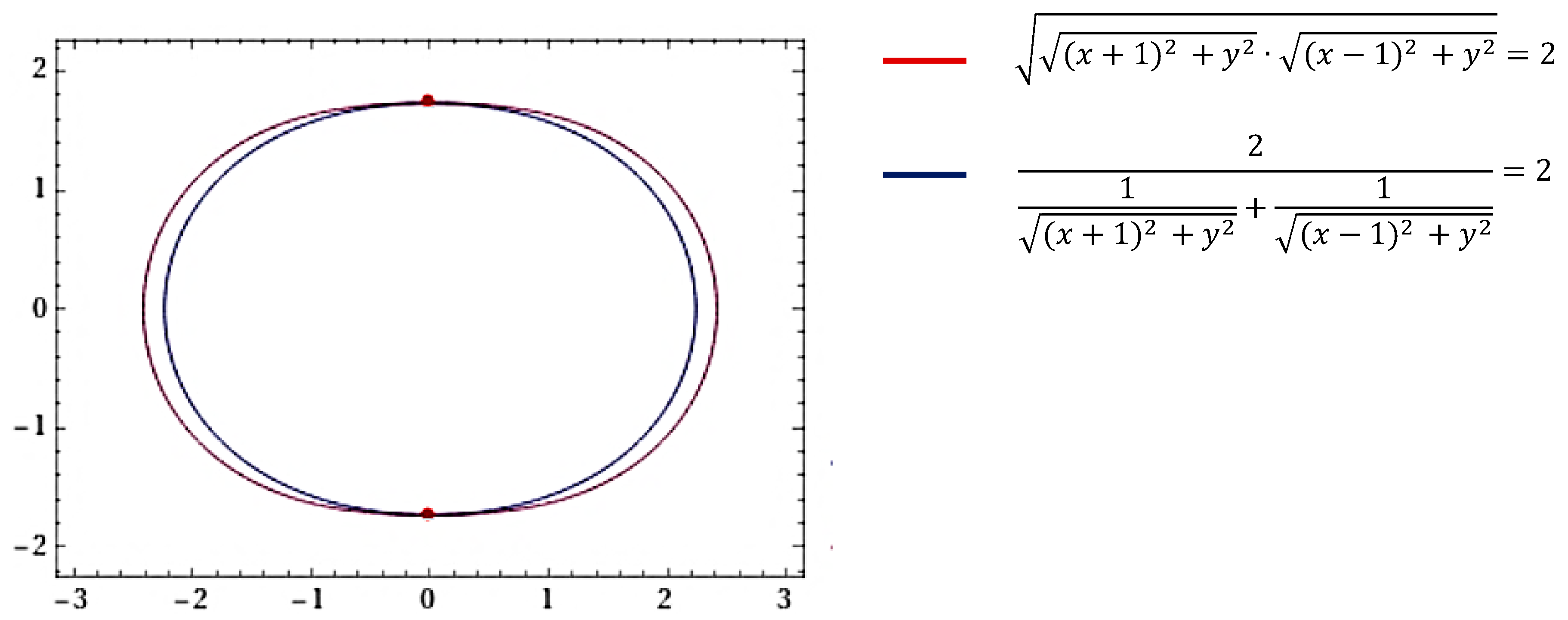
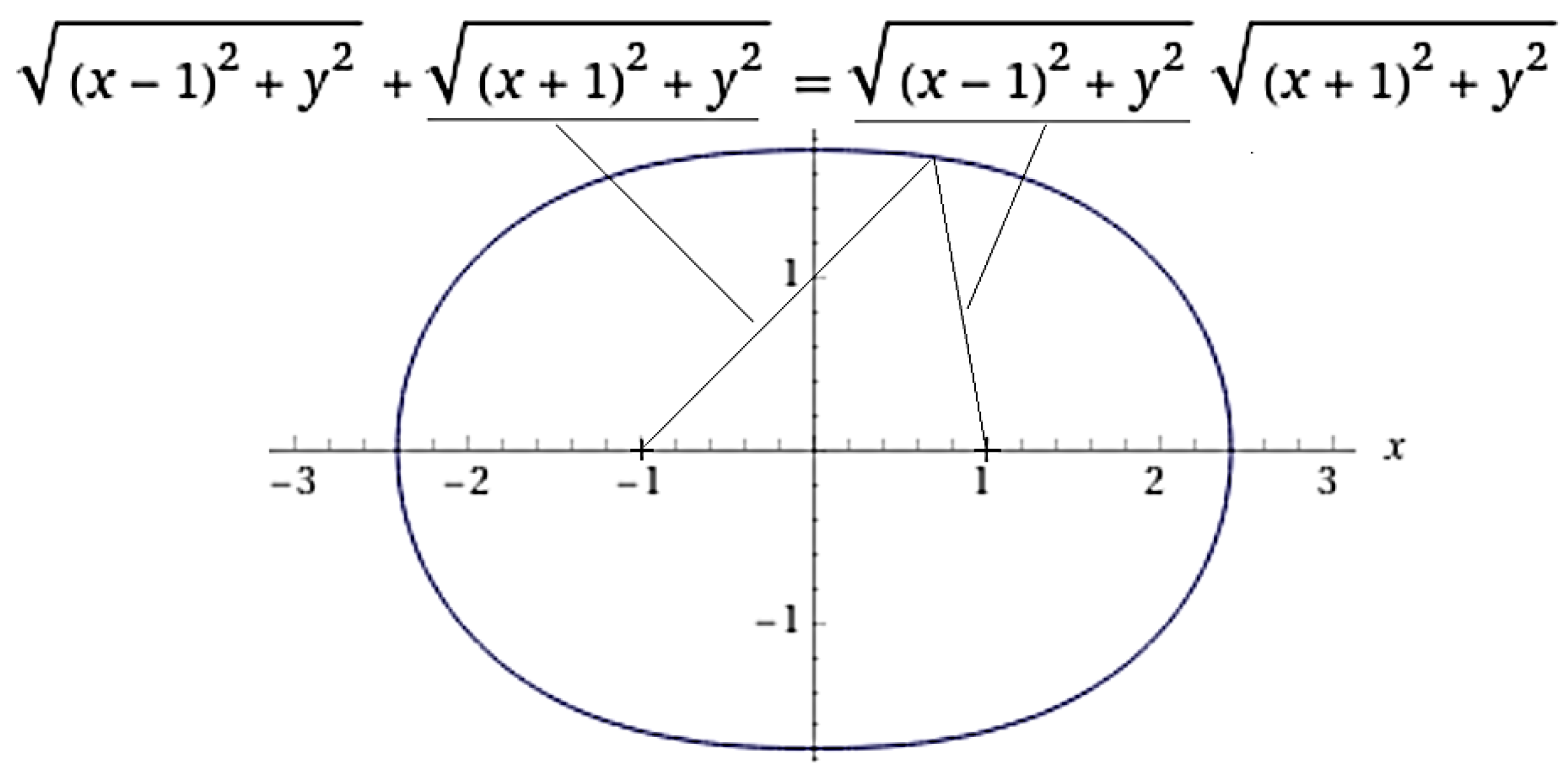
Figure 1 shows an ellipse, a Cassini oval, and a Cayley oval with focal points at (−1,0) and (1,0) for the case of $a=1.1$, which satisfies the following conditions:

$$\begin{array}{l}c<a<c\sqrt{2}-\mathrm{for} \mathrm{Cassini} \mathrm{oval},\\ c<a<c\sqrt{3}-\mathrm{for} \mathrm{Cayley} \mathrm{oval},\end{array}$$

(4)

where $2c=2$—the interfocal distance.

The corresponding equations which describe these curves are also given in Figure 1. The calculations from here to Section 3.5 are performed in Wolfram Mathematica.

At $a=c=1$, the Cassini oval appears as Bernoulli’s lemniscate [29], the Cayley oval also takes a similar form (Figure 2). The ellipse in this case degenerates into a straight-line segment between the focal points.

Cassini oval and Cayley oval can take the form of two other types of curves:

-

at $0<a<c$, the curves are split into two ovals (Figure 3);

-

at $a\ge c\sqrt{2}$ for the Cassini oval and at $a\ge c\sqrt{3}$ for the Cayley oval, curves take the form of a real oval, i.e., a convex closed curve (Figure 4).

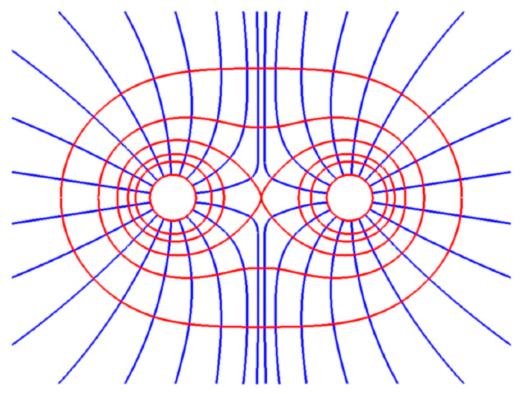
If all variants of Cassini or Cayley ovals are combined in one figure, a picture of equipotential lines of an electrostatic potential created by two equal charges placed at poles (Figure 5) can be obtained [27]. The ellipse equation is of order 2. The equation of a Cassini oval, which is a special case of a Perseus curve, is of order 4. The equation of the Cayley oval is of order 8.

3. Results and Discussion

3.1. Generalized Curves Based on “Power Mean” Concept

The mean of degree p (hereafter, the power mean) for two quantities $r_1$ and $r_2$ is defined by the following equation:

$${\left(\frac{r_1{}^p+r_2{}^p}{2}\right)}^{1/p},$$

(5)

where $p\in \left(-\infty ;+\infty \right).$

It is obvious that $the$ arithmetic mean, geometric mean, and harmonic mean are special cases of the power mean at $p=1,$ $p=0,$ and $p=-1$, respectively.

Using the notion of a power mean to define a symmetric closed curve with two foci similarly to Section 2.1, a family of generalized ovals according to the following equation can be obtained [27]:

$${\left(\frac{r_1{}^p+r_2{}^p}{2}\right)}^{1/p}=a.$$

(6)

For each value of $p\ne \pm \infty ,$ the type of generalized oval is represented by the four types of curves described in Section 2.1, depending on the relation between $a$ and $c$. The curves, which are described by Formula (6) for values $p=-1;0;1;2$ and for the case of $p\to -\infty ;+\infty ,$ will be considered separately.

At $p=1,$ $p=0,$ and $p=-1,$ the curves take the form of ellipse, Cassini oval, and Cayley oval, respectively.

At $p=2$, the curves look like circles with radius $\sqrt{a^2-c^2}$. Figure 6 shows a circle for the case of $c=1, a=\sqrt{2}$, which passes through its focal points.

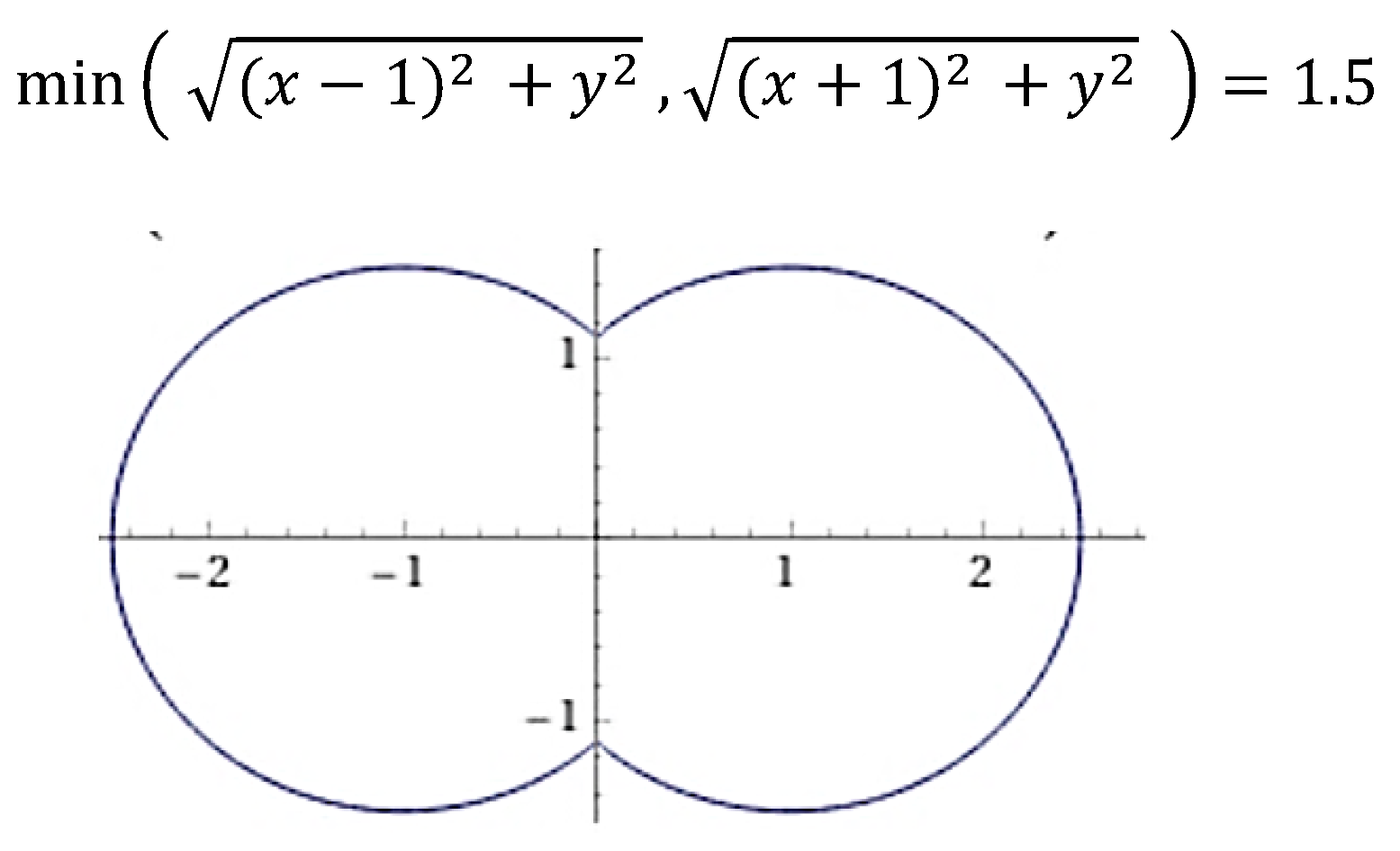
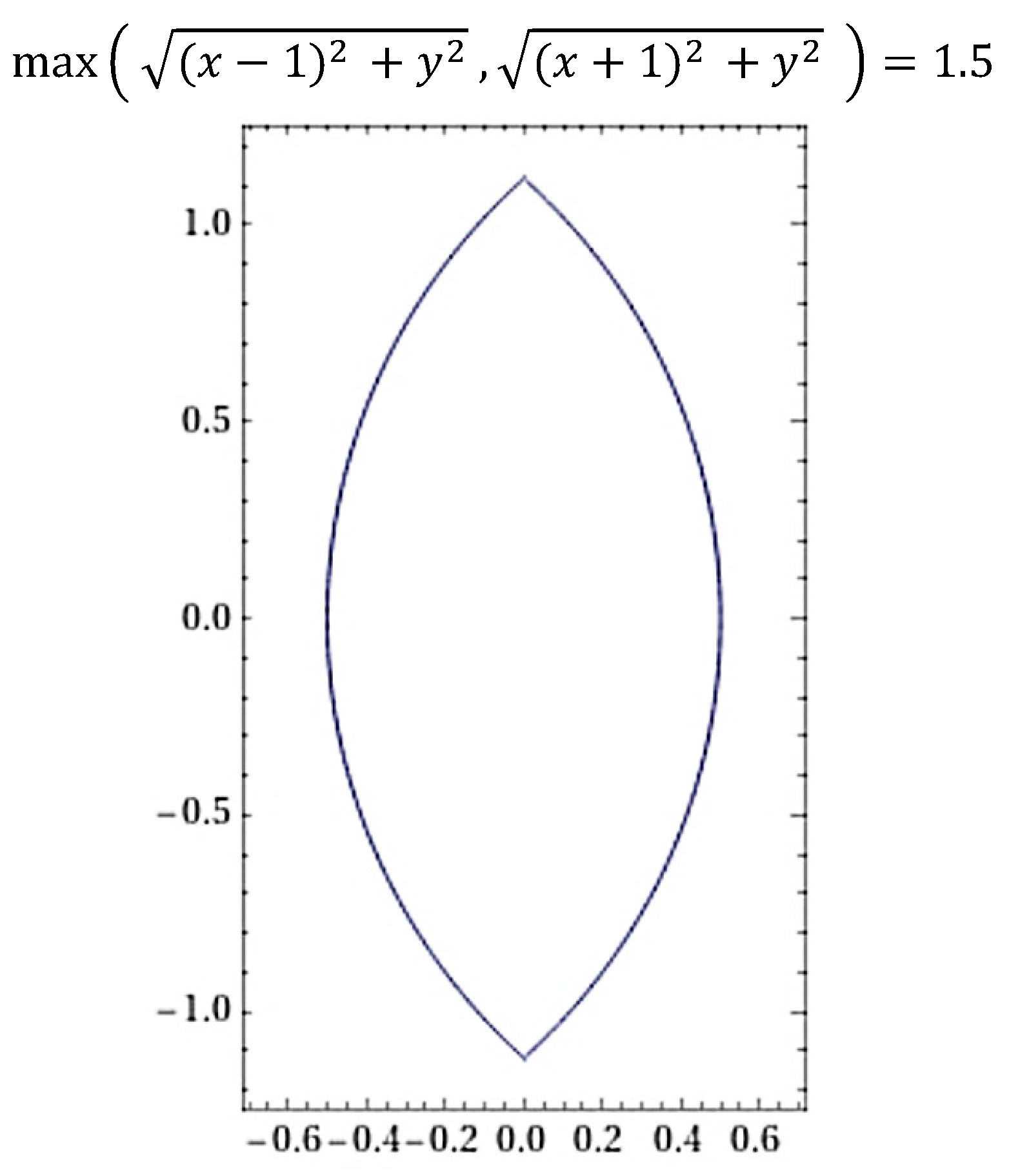
For $p\to -\infty ;+\infty$ the limit of Equation (6) takes the form correspondingly:

$$min\left(r_1, r_2\right)=a; max\left(r_1, r_2\right)=a.$$

(7)

The curves plotted according to Equation (7) are shown in Figure 7 and Figure 8.

The curves in Figure 7 and Figure 8 are not smooth. The two constituent parts of the curve in Figure 8 are extensions of the constituent parts of the curve in Figure 7 to complete circles. The transition between different types of curves when the parameter p is changed can be seen more clearly in the animation (Solved: Tree ovals—mean, gmean & hmean—PTC Community).

3.2. A Special Case of the Cayley Oval

We consider a special case of the Cayley oval with $a=2$. In this case, according to Equation (3), the Cayley oval can be defined as a geometric location of points with the sum of distances from two focal points which equals the product of distances to the foci:

$$r_1+r_2=r_1·r_2.$$

(8)

Figure 9, Figure 10 and Figure 11 show the corresponding curves at $a<c=3, a=c=2$, and $a>c=\sqrt{2}$. The view of the curves corresponds to the types described in Section 2.1.

3.3. Family of Generalized Curves Based on the “Kolmogorov Mean” Concept

Moving on along the path of generalization of the mean notion, the notion of the Kolmogorov mean for two real numbers $r_1, r_2$, defined by the formula can be discussed [30]:

$${\phi }^{-1}\left(\frac{\phi \left(r_1\right)+\phi \left(r_2\right)}{2}\right),$$

(9)

where $\phi \left(x\right)$ is a continuous strictly monotone function.

A family of generalized curves as a geometric place of points defined by the relation can be created:

$${\phi }^{-1}\left(\frac{\phi \left(r_1\right)+\phi \left(r_2\right)}{2}\right)=a.$$

(10)

This family of curves includes the above-described generalized family based on the power average, because if $\phi \left(x\right)=x^p,$ Equation (10) transforms to Equation (5).

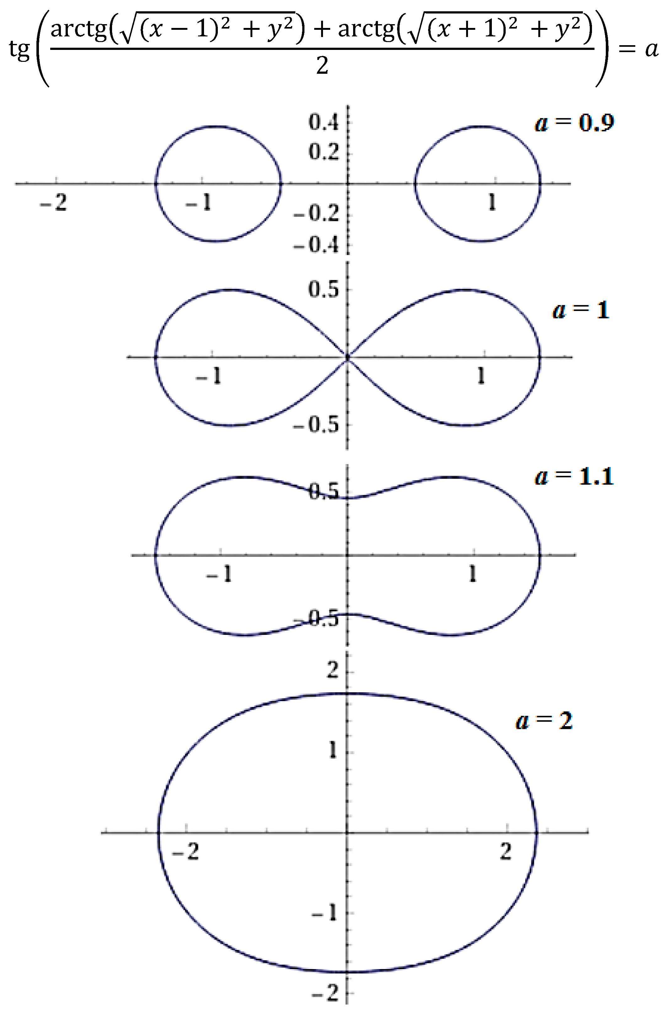
As an example, $\phi \left(x\right)=arctg\left(x\right)$ can be considered. The corresponding family of generalized curves is described by the equation:

$$tg\left(\frac{arctg\left(r_1\right)+arctg\left(r_2\right)}{2}\right)=a.$$

(11)

The family of curves created by Equation (11) corresponds to the four types of curves described in Section 2.1, depending on the ratio of values a and c (Figure 12).

Another example, $\phi \left(x\right)=e^x,$ can be considered. The corresponding family of generalized curves is then described by the equation:

$$ln\left(\frac{e^{r_1}+e^{r_2}}{2}\right)=a,$$

(12)

or after simplifying

$$\frac{e^{r_1}+e^{r_2}}{2}=e^a.$$

(13)

In this case, a family of symmetric closed curves by Equation (13) for $a>c$ (Figure 13 and Figure 14) can be created.

Note that for the inverse case $\phi \left(x\right)=\ln \left(x\right)$, Equation (13) becomes Equation (2), which describes the Cassini ovals.

3.4. Generalized Lemniscates

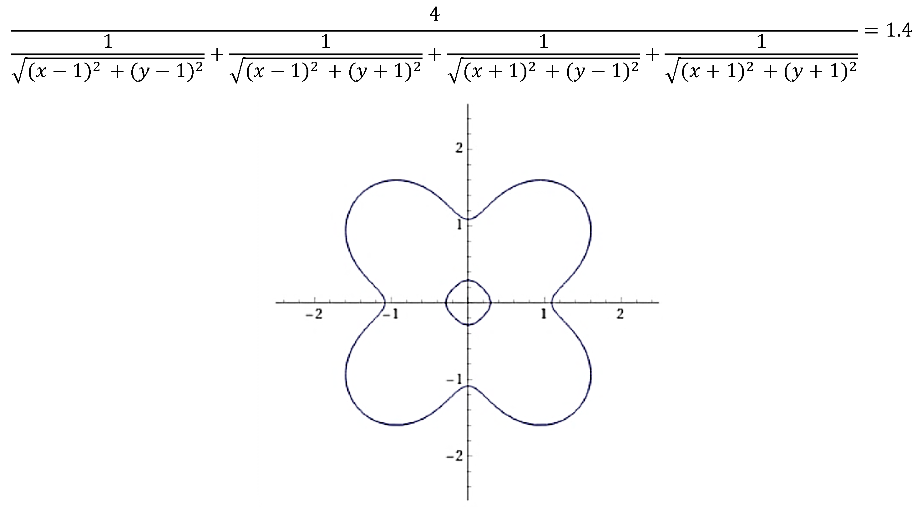
The proposed approach to constructing generalized curves can be extended to multifocal curves. In particular, using the notion of harmonic mean (Equation (3), a family of generalized three-focus lemniscates can be generated:

$$\frac{3}{\frac{1}{r_1}+\frac{1}{r_2}+\frac{1}{r_3}}=a,$$

(14)

where $r_1, r_2, r_3$—distances to the focal points.

Figure 15 shows the corresponding family of curves with focal points at (−1,0), (1,0), and $\left(0,\sqrt{3}\right)$ for different values of a.

A four-focus lemniscate can be constructed in a similar way (Figure 16).

3.5. Construction of Closed Curves by Numerical Methods in Mathcad for 3D Modeling

New families of generalized curves presented above can be widely used for CAD design applications. Hence, a number of practical points should be taken into account. The curves are described by implicitly defined functions, i.e., functions of the form $f\left(x,y\right)=0$, which are difficult to resolve with respect to one of the variables. As mentioned in the introduction, such an analytical description is unsuitable for CAD design, because the curves (surfaces) are to be represented in:

-

in polar (cylindrical) coordinates;

-

in parametric form;

-

in the form of numerical data set, by which an approximation curve will be built.

A number of curves, particularly the widely studied Cassini ovals, can be described in polar coordinates [21]:

$${\rho }^4-2c^2{\rho }^2\cos \left(2\phi \right)=a^4-c^4.$$

(15)

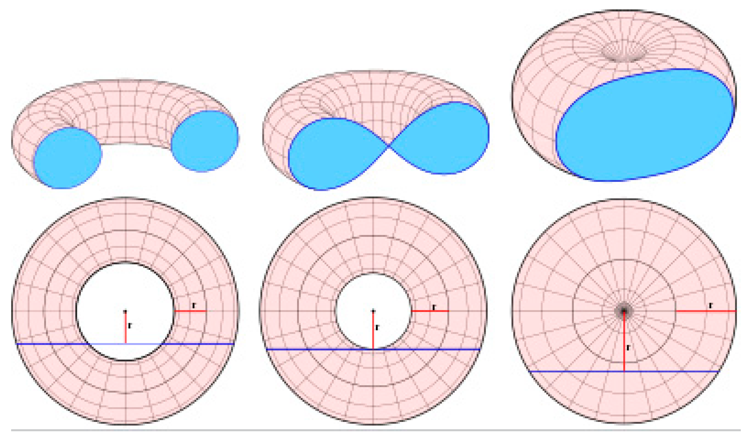
In addition, the Cassini ovals as a special case of the Perseus curves can be constructed as sections of the torus by a plane [17] (Figure 17).

Obtaining equations in polar coordinates for generalized curves considered above (e.g., Cayley ovals of order 8, curves based on the Kolmogorov mean, multifocal lemniscates of orders 6 and 8) can be very time-consuming and, additionally, is not justified in terms of achieving the necessary accuracy of curve description, providing inevitable errors in real production or 3D printing.

It is important to develop a numerical method for the generation of such curves, which enables obtaining an array of data containing curve coordinates. These data can be exported to CAD systems, in particular Creo, for approximation using B-splines.

The authors propose a universal numerical method for constructing such curves with the required accuracy. The method is based on the principles of the marching cubes algorithm [31].

An implicitly given function may be described by the equation:

$$f\left(x,y\right)=0.$$

(16)

In this case, a graph of such a function in xyz coordinates is a projection of the surface $f\left(x,y\right)$ on the plane $z=0$. This graph can be obtained Mathcad by means of the Contour Plot tool, which can be applied to the surface in the graphical shell 3D Plot [8].

Then the problem is reduced to finding the geometric place of points $\left(x,y\right)$ on plane $z=0$, which satisfies Equation (16). The following algorithm is proposed for finding such points.

The variation range of the variables $x,y$, based on the available function graph (16), is determined, and step $h$ is set. An external loop for the variable $x$ in a given range is provided with step $h$, as well as an internal loop for the variable $y$ in the given range with a much smaller step, for example, $0.01 h$.

Calculated values $f\left(x_i,y_j\right)$ at each step of the loop can be sequentially determined in which the roots of Equation (16) are located. As an indication of their location in a current interval $\left((x_i,y_{j-1}), \left(x_i,y_j\right)\right)$, an expression is used:

$$f\left(x_i,y_{j-1}\right)f\left(x_i,y_j\right)<0.$$

(17)

where $i,j$ are step numbers, with the intervals $\left((x_i,y_{j-1}), \left(x_i,y_j\right)\right)$.

The following points are considered $\left(x_i,y_j-0.01 h/2\right)$ as an approximate root of Equation (16).

The calculated approximate roots $\left(x,y\right)$ are recorded in a two-dimensional array $R_y.$ Then the described procedure is repeated for the replacement case of the variables $x,y$ in the inner and outer loops. The resulting data can also be written to the two-dimensional array $R_x$.

Finally, the two resulting arrays of points $\left(x,y\right)$ are combined into the array $R=R_y{\displaystyle \cup }{R}_x$, which is a numerical representation of the implicit function (16). The graph of such a numerically given function can be plotted with standard means of the mathematical package.

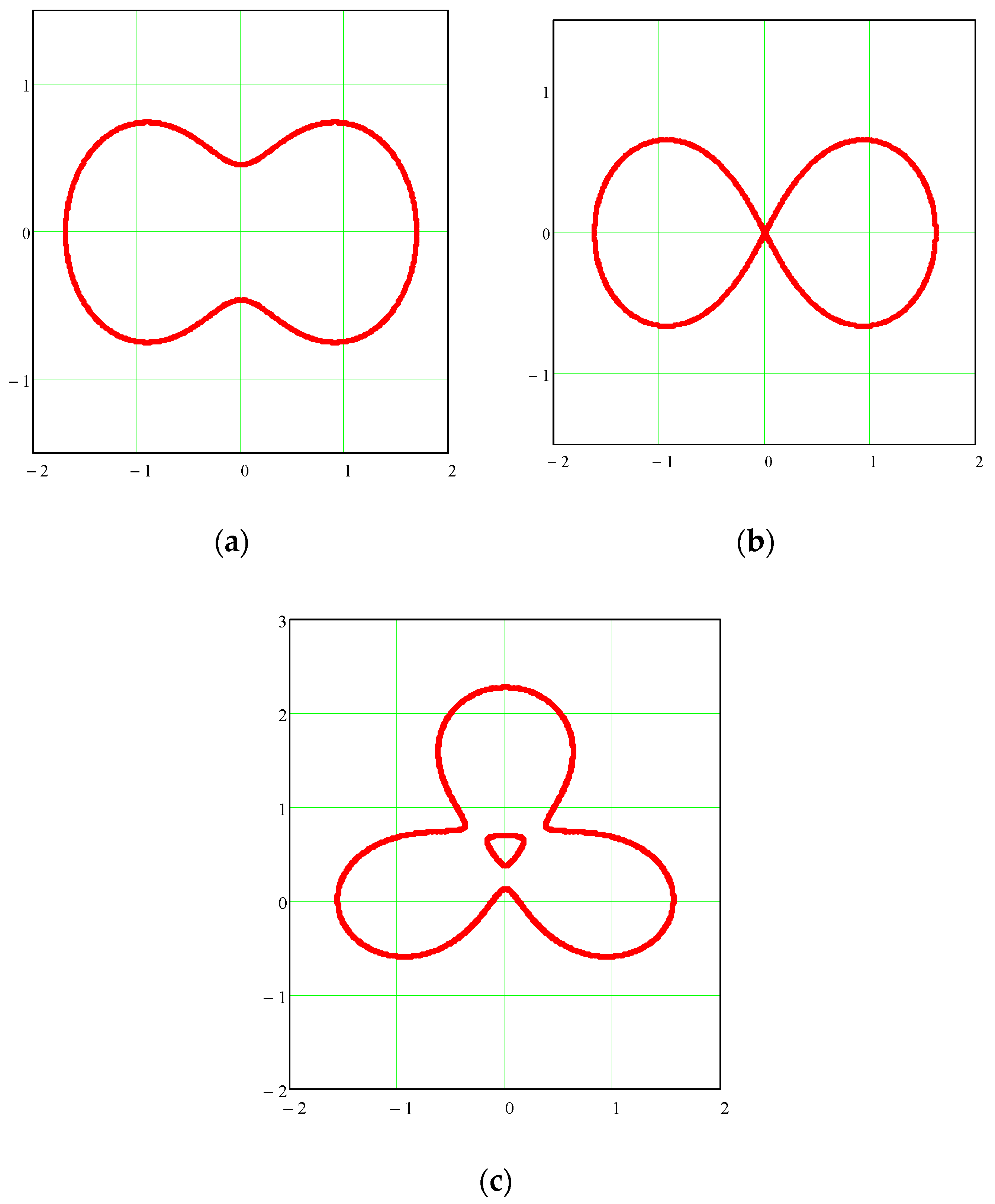
The proposed method is implemented in Mathcad. Mathcad was chosen as preferable because it is integrated into the CAD system PTC Creo [8]. Examples of generalized curves in the Mathcad environment are shown in Figure 18.

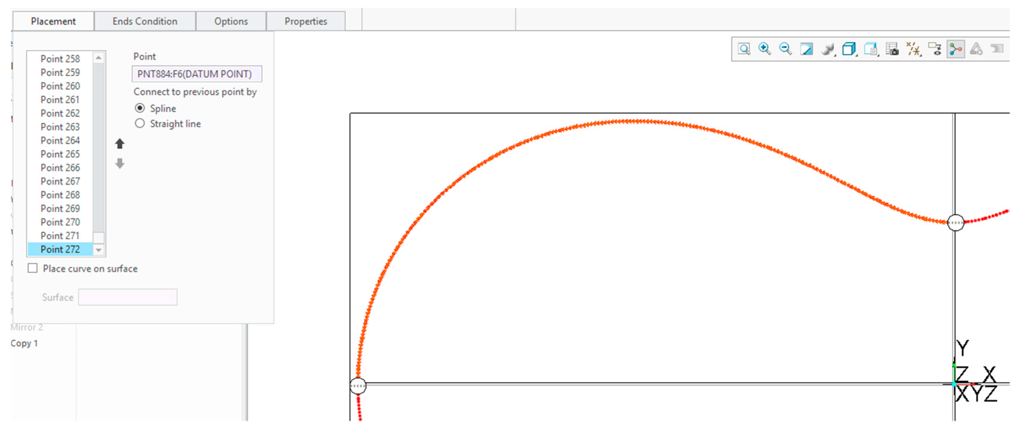
The application of the obtained numerical data for geometric modeling is considered below. The data are to be exported to the Creo CAD system and then approximated with B-splines. The approximation algorithm can be examined on the Cayley oval, shown in Figure 18a. The numerical interpretation of this curve consists of 1092 points exported to Creo. Since the figure has two symmetry axes, only the quarter defined by 273 points is estimated. The approximation by standard Creo instruments is shown in Figure 19.

However, control of the curvature profile shows an unsatisfactory result (Figure 20a). The approximation is characterized by a random change in the curvature sign, which does not correspond to the true function $f\left(x,y\right)$ (see scaled-up view of a part of the curve, Figure 20b).

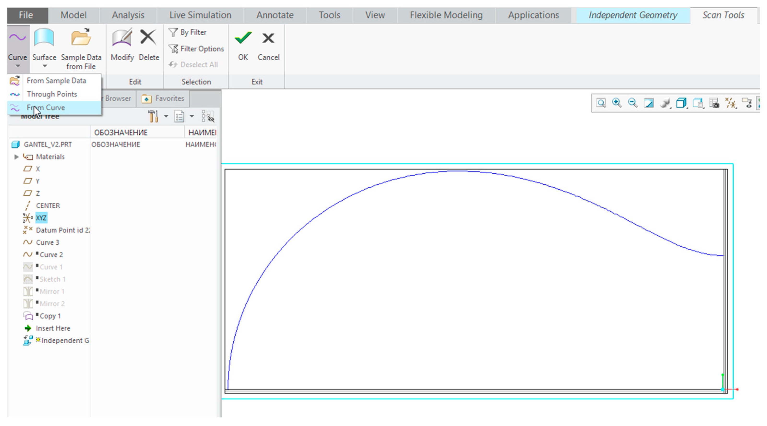
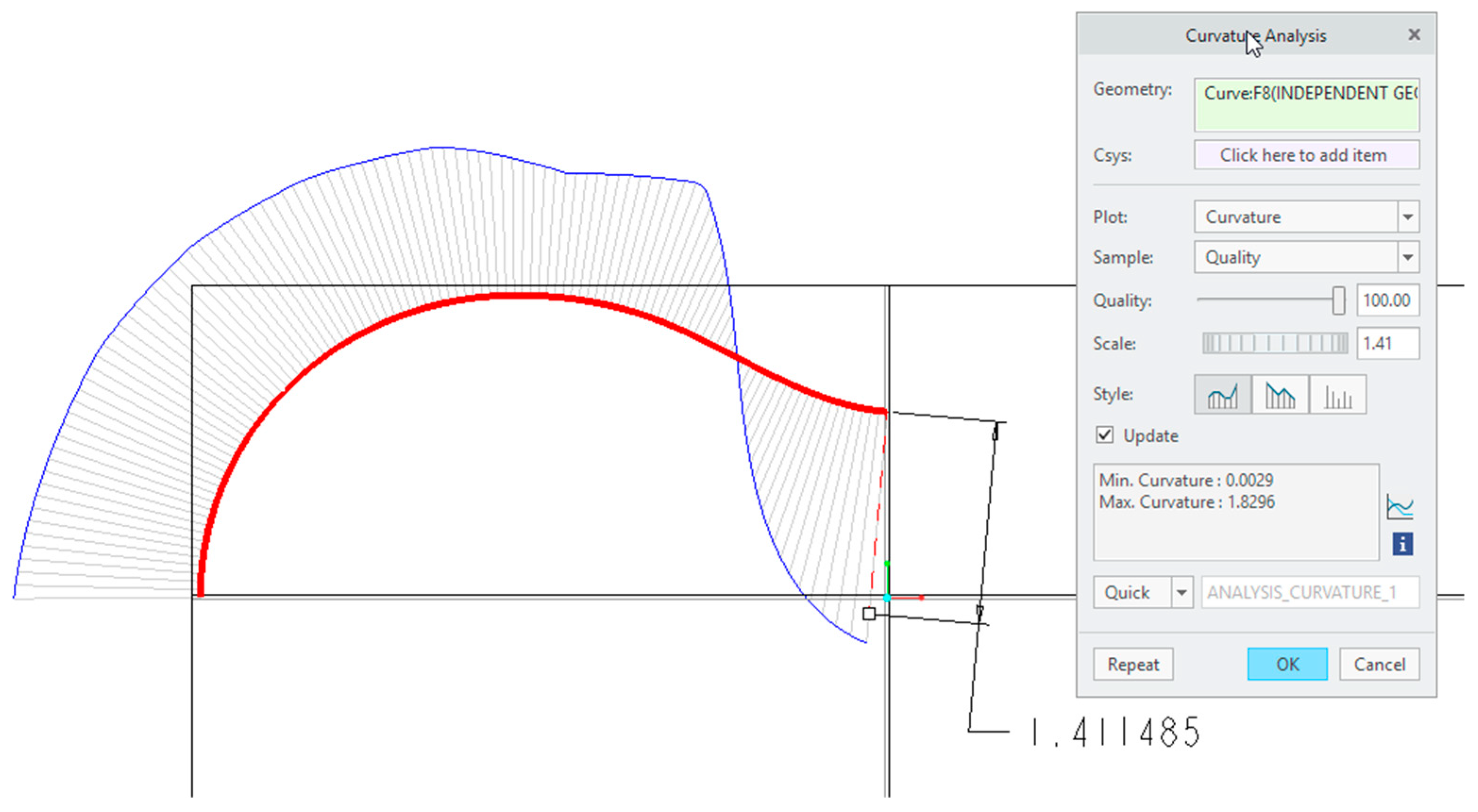
It is necessary to reduce the number of points the approximating function graph goes through, and to use Scan Tools and Independent Geometry tools [8]. Figure 21 shows the approximating function created with 20 points, and Figure 22 shows the curvature corresponding to it.

Obviously, the profile of curvature is smooth in this case. Thus, the maximum deviation of the approximating function from the original numerical data is 0.0013 mm (Figure 23) or 0.18%.

It is possible to control the curvature at high approximation accuracy by choosing the optimal number of plotting points. Figure 24 shows the final approximation for the entire figure (corresponding graph in Mathcad—Figure 18a). Other examples of generalized curves (Figure 18b,c), prepared in Creo, are shown in Figure 25.

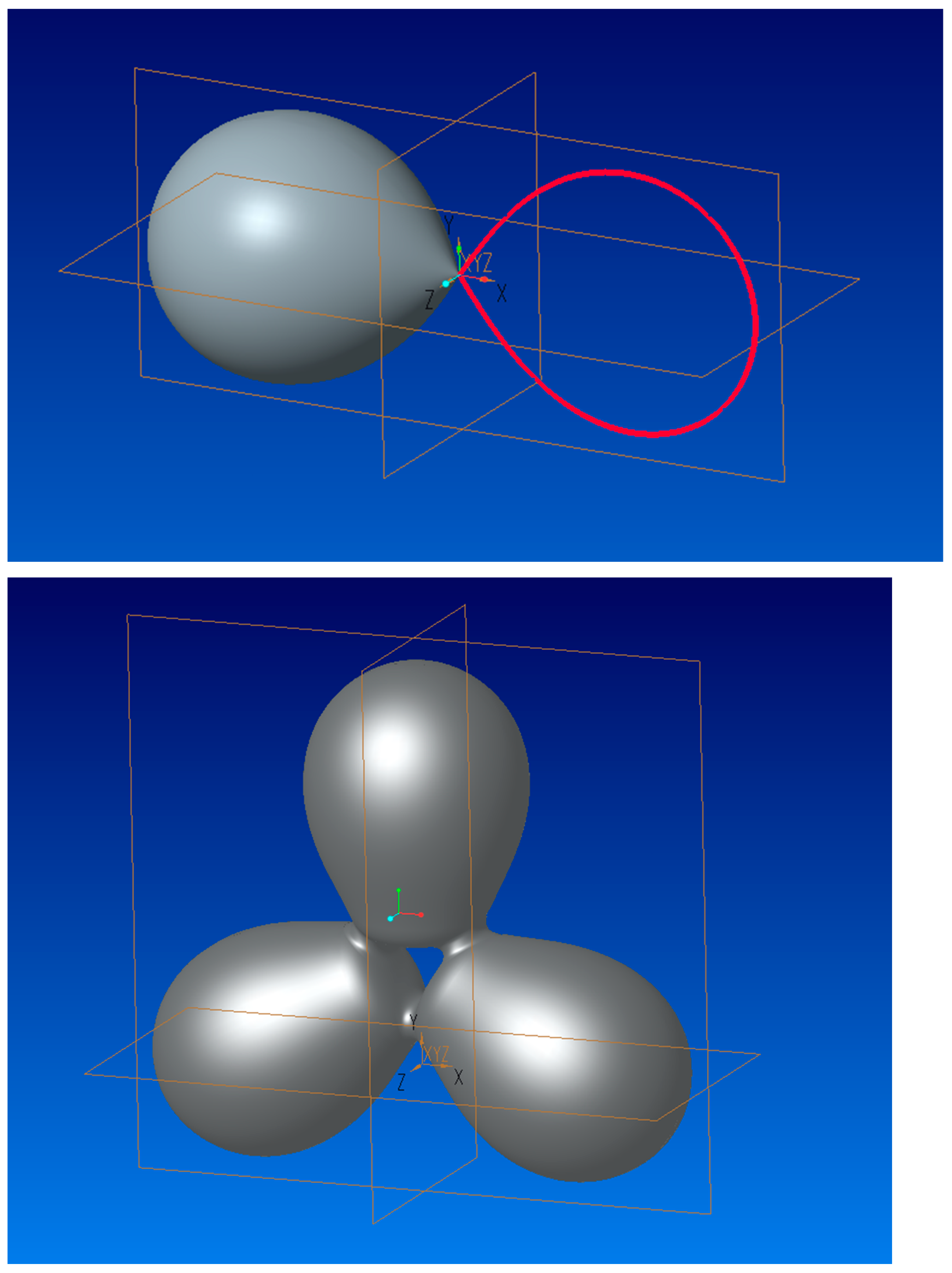
The application of CAD systems provides a great opportunity for the 3D modeling of such curves with further 3D printing. Figure 26 shows 3D interpretations of the flat curves shown in Figure 25.

4. Conclusions

The generation of symmetric closed curves with two or more foci is of particular practical interest. Such curves can be applied to radiolocation, group theory, cluster analysis, engineering and construction design, and quantum physics.

An approach based on the application of different notions of “mean” (in particular, the Kolmogorov mean) is proposed, which allows:

-

description in unified new terms of the known types of flat symmetric closed curves with two focal points (e.g., second-order curves (ellipse), fourth-order curves (Cassini oval));

-

identification of new classes of curves (e.g., eighth-order curves (generalized Cayley ovals), generalized multifocal lemniscates of the sixth and eighth orders).

A universal numerical method to construct such curves using common mathematical packages is developed. Approximation of the obtained numerical data for geometrical design by means of B-splines in Creo is considered. The applicability of the method is demonstrated, as well as the possibility to provide high smoothness of curvature profiles and given modeling accuracy. Illustrative examples of curves and 3D surfaces, based on the proposed approach, are given.

References

1. Gibson, I.; Rosen, D.W.; Stucke, B. Additive Manufacturing Technologies: 3D Printing, Rapid Prototyping, and Direct Digital Manufacturing, 2nd ed.; Springer: New York, NY, USA, 2015. [Google Scholar]
2. Chong, L.; Ramakrishna, S.; Singh, S. A review of digital manufacturing-based hybrid additive manufacturing processes. Int. J. Adv. Manuf. Technol. 2018, 95, 2281–2300. [Google Scholar] [CrossRef]
3. Lee, M.; Fang, Q.; Cho, Y.; Ryu, J.; Liu, L.; Kim, D. Support-free hollowing for 3D printing via Voronoi diagram of ellipses. Comput. Aided Des. 2018, 101, 23–36. [Google Scholar] [CrossRef]
4. Qin, Y.; Qi, Q.; Scott, P.J.; Jiang, X. Status, comparison, and future of the representations of additive manufacturing data. Comput. Aided Des. 2019, 111, 44–64. [Google Scholar] [CrossRef]
5. Ziatdinov, R.; Muftejev, V.G.; Akhmetshin, R.I.; Zelev, A.P.; Nabiyev, R.I.; Mardanov, A.R. Universal software platform for visualizing class F curves, log-aesthetic curves and development of applied CAD systems. Sci. Vis. 2018, 10, 29–47. [Google Scholar] [CrossRef]
6. Wo, M.S.; Gobithaasan, R.U.; Miura, K.T. Log-aesthetic magnetic curves and their application for CAD systems. Math. Probl. Eng. 2014, 2014, 504610. [Google Scholar] [CrossRef] [Green Version]
7. Haron, H.; Rehman, A.; Adi, D.; Lim, S.P.; Saba, T. Parameterization Method on B-Spline Curve. Math. Probl. Eng. 2012, 2012, 640472. [Google Scholar] [CrossRef] [Green Version]
8. Vilau, C.; Balc, N.; Leordean, D.; Cosma, C. Static analysis to redesign the gripper, using CREO parametric software tools. Acad. J. Manuf. Eng. 2015, 13, 77–82. [Google Scholar]
9. Meek, D.; Walton, D. The use of Cornu spirals in drawing planar curves of controlled curvature. J. Comput. Appl. Math. 1989, 25, 69–78. [Google Scholar] [CrossRef] [Green Version]
10. Farin, G. Class A Bézier curves. Comput. Aided Geom. Des. 2006, 23, 573–581. [Google Scholar] [CrossRef]
11. Barton, M.; Gershon, E. Spiral fat arcs—Bounding regions with cubic convergence. Graph. Models 2011, 73, 50–57. [Google Scholar] [CrossRef]
12. Levien, R.; Séquin, C. Interpolating Splines: Which is the fairest of them all? Comput. Aided Des. Appl. 2009, 6, 91–102. [Google Scholar] [CrossRef] [Green Version]
13. Yoshida, N.; Saito, T. Interactive aesthetic curve segments. Vis. Comput. 2006, 22, 896–905. [Google Scholar] [CrossRef]
14. Plaumann, D.; Sturmfels, B.; Vinzant, C. Quartic curves and their bitangents. J. Symb. Comput. 2010, 46, 712–733. [Google Scholar] [CrossRef] [Green Version]
15. Rakcheeva, T. Polypolar coordination and symmetries. Comput. Res. Modeling 2010, 2, 329–341. (In Russian) [Google Scholar] [CrossRef] [Green Version]
16. Ochkov, V.; Nori, M.; Borovinskaya, E.; Reschetilowski, W. A new ellipse or math Porcelain service. Symmetry 2019, 11, 184. [Google Scholar] [CrossRef] [Green Version]
17. Krivoshapko, S.N.; Ivanov, V.N. Encyclopedia of Analytical Surfaces; Springer International Publishing: Cham, Switzerland, 2015; 752p. [Google Scholar]
18. Ochkov, V. 25 Problems for STEM Education; Chapman and Hall/CRC: London, UK, 2020. [Google Scholar]
19. Stillwell, J. Mathematics and His History; Springer: Cham, Switzerland, 2010. [Google Scholar]
20. Darling, D. The Universal Book of Mathematics: From Abracadabra to Zeno’s Paradoxes; John Wiley & Sons: Hoboken, NJ, USA, 2004. [Google Scholar]
21. Ivanov, V. Cassini oval, lemniscate curve and lemniscate surfaces. Struct. Mech. Eng. Constr. Build. 2014, 5, 3–9. (In Russian) [Google Scholar]
22. Grabusts, P. Different approaches to clustering—Cassini ovals. Inf. Technol. Manag. Sci. 2017, 20, 30–33. [Google Scholar] [CrossRef] [Green Version]
23. Inoguchi, J. Attractive plane curves in differential geometry. In Mathematical Progress in Expressive Image Synthesis, 3rd ed.; Mathematics for Industry; Springer: Singapore, 2016; Volume 24, pp. 121–135. [Google Scholar]
24. Mohapatra, M.; Sahoo, S. Mapping properties of a scale invariant Cassinian metric and a Gromov hyperbolic metric. Bull. Aust. Math. Soc. 2018, 97, 141–152. [Google Scholar] [CrossRef] [Green Version]
25. Kargar, R.; Ebadian, A.; Sokól, J. On Booth lemniscate and starlike functions. Anal. Math. Phys. 2019, 9, 143–154. [Google Scholar] [CrossRef]
26. Lawrence, D. A Catalog of Special Plane Curves; Dover Publications, Inc.: New York, NY, USA, 2014. [Google Scholar]
27. Cayley Oval. Available online: https://mathcurve.com/courbes2d.gb/cayleyovale/cayleyovale.shtml (accessed on 18 October 2021).
28. Perrard, S.; Labousse, M.; Miskin, M.; Fort, E.; Couder, Y. Self-organization into quantized eigenstates of a classical wave-driven particle. Nat. Commun. 2014, 5, 3219. [Google Scholar] [CrossRef] [Green Version]
29. Langer, J.C.; Singer, D.A. Reflections on the lemniscate of Bernoulli: The forty-eight faces of a mathematical gem. Milan J. Math. 2010, 78, 643–682. [Google Scholar] [CrossRef]
30. Kolmogorov, A.; Fomin, S. Elements of the Theory of Functions and Functional Analysis; Volume 1; Metric and Normed Spaces; Graylock Press: Rochester, NY, USA, 1957. [Google Scholar]
31. Lorensen, W.; Johnson, C.; Kasik, D.; Whitton, M. History of the marching cubes algorithm. IEEE Comput. Graph. Appl. 2020, 40, 8–15. [Google Scholar] [CrossRef] [PubMed]
Figure 1. Ellipse, Cassini oval, Cayley oval at c < a < c 2 .
Mathematics 09 03325 g001
Figure 2. Cassini oval, Cayley oval at c = a .
Mathematics 09 03325 g002
Figure 3. Cassini oval, Cayley oval at 0 < a < c .
Mathematics 09 03325 g003
Figure 4. Cassini oval, Cayley oval at a c 3 .
Mathematics 09 03325 g004
Figure 5. Combination of Cassini and Cayley ovals—the electrostatic field lines.
Mathematics 09 03325 g005
Figure 6. Generalized curve (circle) at p = 2 ,   c = 1 ,   a = 2 .
Mathematics 09 03325 g006
Figure 7. Generalized curve at p .
Mathematics 09 03325 g007
Figure 8. Generalized curve at p + .
Mathematics 09 03325 g008
Figure 9. A particular case of the Cayley oval at a < c = 3 .
Mathematics 09 03325 g009
Figure 10. A particular case of the Cayley oval at a = c = 2 .
Mathematics 09 03325 g010
Figure 11. A particular case of the Cayley oval at a > c = 2 .
Mathematics 09 03325 g011
Figure 12. The generalized oval constructed for φ ( x ) = a r c t g ( x ) .
Mathematics 09 03325 g012
Figure 13. The generalized oval constructed for φ ( x ) = e x ,   a = 2 , c = 1 .
Mathematics 09 03325 g013
Figure 14. The generalized oval constructed for φ ( x ) = e x ,   a = 0.6 ,   c = 0.5 .
Mathematics 09 03325 g014
Figure 15. Generalized three-focus lemniscates.
Mathematics 09 03325 g015
Figure 16. Generalized four-focus lemniscate.
Mathematics 09 03325 g016
Figure 17. Cassini ovals as cross-sections of the torus with a plane.
Mathematics 09 03325 g017
Figure 18. Cayley oval (a), Cayley lemniscate (b), a three-focus lemniscate (c) constructed in Mathcad.
Mathematics 09 03325 g018
Figure 19. An approximating function which goes through all points.
Mathematics 09 03325 g019
Figure 20. A profile of curvature for the approximating function which goes through all points: (a) general view; (b) scaled-up view of a part of the curve.
Mathematics 09 03325 g020
Figure 21. Approximating function which passes through 20 points.
Mathematics 09 03325 g021
Figure 22. Profile of curvature for approximating function which passes through 20 points.
Mathematics 09 03325 g022
Figure 23. The variance graph for the approximating function with 20 points.
Mathematics 09 03325 g023
Figure 24. Cayley oval constructed in Creo.
Mathematics 09 03325 g024
Figure 25. Cayley lemniscate (left) and a three-focus lemniscate constructed in Creo (right).
Mathematics 09 03325 g025
Figure 26. 3D modeling in Creo.
Mathematics 09 03325 g026
Publisher’s Note: MDPI stays neutral with regard to jurisdictional claims in published maps and institutional affiliations.