A Bayesian Model of COVID-19 Cases Based on the Gompertz Curve

Abstract

The COVID-19 pandemic has highlighted the need for finding mathematical models to forecast the evolution of the contagious disease and evaluate the success of particular policies in reducing infections. In this work, we perform Bayesian inference for a non-homogeneous Poisson process with an intensity function based on the Gompertz curve. We discuss the prior distribution of the parameter and we generate samples from the posterior distribution by using Markov Chain Monte Carlo (MCMC) methods. Finally, we illustrate our method analyzing real data associated with COVID-19 in a specific region located at the south of Spain.

1. Introduction

In December 2019, the number of pneumonia cases inexplicably increased in China. Later, scientists discovered that they were caused by a novel kind of coronavirus, called SARS-CoV-2, which appeared for the first time in Wuhan, China, see [1,2]. From that date, the disease began spreading in a huge number of countries and regions outside China where have confirmed new cases and deaths almost every day. The COVID-19, the disease related to this new coronavirus, has had a huge impact in human health and social life all over the world, even more than some other infectious diseases occurred in recent years. At the time the paper was submitted, it had already affected $68.31$ millions of people with $1.56$ millions of deaths (taken from Our World in Data, https://ourworldindata.org/). In fact, COVID-19 has become an important risk factor of mortality currently around the world.

Due to the impact on health, society and economy there is a need to find mathematical models that lead us to understand the evolution of that disease and evaluate if a particular policy has been successful in achieving the intended outcomes, e.g., to reduce the infections. It is well-known that the infectious disease transmission is a complex diffusion process due to social relationships. Different models have been widely developed in the literature to study the transmission process of infectious diseases theoretically, that allows us accurately predict the future development trend of infectious diseases, see among others [3,4,5,6,7,8,9,10]. While the traditional epidemiological models describe the dynamic behavior of the diseases through differential equations allowing the laws of transmission within the population, the statistic models (also so-called phenomenological models) which follow certain laws of epidemiology [9,11], are widely used in real-time forecasting for infection trajectory or size of epidemics in early stages of pandemic [12,13].

The main objective of this paper is to develop a model for the cumulative number of COVID-19 cases from a Bayesian perspective. Once the model is fitted, we will be able to make predictions to evaluate the trend of new infected cases. Bayesian methods provide an excellent theoretical framework for analyzing experimental data and the main key of its success lies on its ability to incorporate prior knowledge about the quantity of interest as a distribution function. In this case, there exists a lot of information about the new coronavirus during the pandemic which is worth to take into account as well as the behaviour of other types of coronavirus.

The goal of the Bayesian approach is to learn about the parameters which describe our phenomenon of interest by taking into account different sources of information. Often, the decision makers have access to external information such as expert views and past studies or data from other locations. This previous knowledge is incorporated into the Bayesian analysis as the prior distribution. It is well known that the prior distribution leads in general to a better estimation of the quantity under study, when it is used together with experimental data. Thorough reviews of the Bayesian approach can be found in [14,15,16].

Let $\left[X\right|\Theta =\theta ]=X_{\theta }$ be the underlying observation having a probability density function (PDF), $p_{\theta }\left(x\right)$, where $\theta$ means the unknown parameter belonging to the parameter space $\Theta \subseteq {\mathbb{R}}^n$, $n\in \mathbb{N}$, $n\ge 1$. As explained above, under the Bayesian approach, prior beliefs about parameters are combined with sample information based on the experience from a sample $x=(x_1,\dots ,x_n)$ of the variable $X_{\theta }$ by using the Bayes theorem.

Let $\pi$ be the prior belief on $\Theta$ which incorporates our beliefs about the parameter $\theta$ before any data observation. It is also common to denote by $\pi \left(\theta \right)$ the PDF of a particular prior distribution $\pi$. In literature, it is possible to find that prior distributions can be obtained using many methods. It is remarkable that, in general, it is not easy to find the best way to express the prior information as a prior distribution function. However, insightful choice of prior may be crucial for obtaining a proper estimate of the posterior.

At this point and based on a sample of the underlying distribution, $x=\{x_1,\dots ,x_n\}$, jointly with the prior density, $\pi \left(\theta \right)$, and Bayes’ theorem we obtain the posterior distribution, denoted by ${\pi }_x$, as a random variable having the following PDF

$${\pi }_x\left(\theta \right)=\pi \left(\theta \right|x)=\frac{l\left(\theta \right|x\left)\pi \right(\theta )}{m_{\pi }\left(x\right)},$$

(1)

where $l\left(\theta \right|x)$ denotes the likelihood function of the sample and $m_{\pi }\left(x\right)$ denotes the marginal density given by

$$m_{\pi }\left(x\right)={\int }_{\Theta }l\left(\theta \right|x)\pi \left(\theta \right)d\theta .$$

Just as the prior distribution $\pi$ reflects the knowledge about $\theta$ before any experimentation, so ${\pi }_x$ reflects the update belief about $\theta$ after having a sample x. That means that the posterior distribution mixes the prior belief with the information contained in the sample about $\theta$. For further information see [14]. Finally, the posterior distribution can be used to solve all standard statistical problems, like point and interval estimation, hypothesis testing and predictions. Recently, we find a rapid increase in the number of publications related to model COVID-19 using Bayesian techniques in literature, see for example [17,18,19,20,21].

2. The Model

Our interest is focused on finding a probabilistic model to describe the evolution of the SARS-CoV-2 in a specific region and forecast the number of new cases in near future time intervals from a Bayesian perspective. Based on the interpretation of the model as a complex system, we assume the total number of infections experienced up to time t is a non-homogeneous Poisson process (NHPP) denoted by $\left\{N\right(t),t\ge 0\}$. One of the main issue in the NHPP model is to determine an appropriate intensity function, $\lambda (·)$, which leads us to an increasing and invertible mean value function representing the expected number of infections experienced up to t, i.e.,

$$\Lambda \left(t\right)=E\left[N\left(t\right)\right]={\int }_0^t\lambda \left(x\right)dx.$$

Further details on the statistical analysis and NHPPs can be found in [22,23] and a comprehensive catalogue of intensity functions is given in [24].

For the purpose of this work, we will consider the classical Gompertz curve to explain the cumulative number of new cases. Our choice is based on the intuitive biological interpretation of its parameters and the fact that this curve is widely used in growth analysis in Biology. Additionally, the Gompertz curve is of particular interest to describe a growth curve for population studies in situations where growth is not symmetrical about the point of infection, see [25,26,27,28], for further information about the Gompertz model. Moreover, the Gompertz curve have been widely used in epidemiology and virology to explain the behaviour of many biological processes, see for example [29,30,31,32]. Concerning to the COVID-19 we refer the readers to [33,34,35,36,37,38]. Finally, we also recommend readers see [39] where authors propose a generalized Gompertz growth model. Remarking its limitations we will find that the Gompertz model does not address the core issues of epidemiological models, namely, the well-mixing hypothesis and lack of spatial influences.

Among the different reparameterisations we find in literature we will consider the following expression of the Gompertz curve given by

$$g\left(t\right|\mathbf{\theta })=aexp(-bexp(-ct)),\mathbf{\theta }=(a,b,c)\in {\mathbb{R}}^{+}\times {\mathbb{R}}^{+}\times {\mathbb{R}}^{+},$$

(2)

where t represents the time since the first case of infection and a, b and c are parameters having a biological interpretation. A detailed interpretation of those parameters can be found in [33]. To sum up, a represents the upper asymptote of infections and also determines the area under the curve $\partial g\left(t\right|\mathbf{\theta })/\partial t$, b sets the displacement along the time and it is related with the initial cases at time zero, $g\left(0\right|\mathbf{\theta })$, and also determines the location of the maximum on the time axis, $t_{max}=ln\left(b\right)/c$, as we will discuss later on. Finally, c is a coefficient that determines the exponential decay rate of the relative growth rate of $g\left(t\right)$, i.e.,

$$\frac{1}{g\left(t\right|\mathbf{\theta })}\frac{\partial g\left(t\right|\mathbf{\theta })}{\partial t}=cbexp(-ct).$$

It is also worth mentioning that $1/c$ measures the width (duration) of the curve, see [33] for further information.

It is clear that the Gompertz curve considers some initial counts at time zero and also we should take in account that $N\left(0\right)$ is assumed to be zero in a NHPP process. Therefore, in order to avoid the problem of detecting the initial moment, in other words the disease initial outbreak, we will consider

$$\Lambda \left(t\right|\mathbf{\theta })=g\left(t\right|\mathbf{\theta })-g\left(0\right|\mathbf{\theta }),\mathbf{\theta }=(a,b,c)\in {\mathbb{R}}^{+}\times {\mathbb{R}}^{+}\times {\mathbb{R}}^{+}.$$

(3)

A straightforward computation shows that the intensity function is given by

$$\lambda \left(t\right|\mathbf{\theta })=\frac{\partial \Lambda \left(t\right|\mathbf{\theta })}{\partial t}=\frac{\partial g\left(t\right|\mathbf{\theta })}{\partial t}=abcexp(-bexp(-ct)-ct),\mathbf{\theta }=(a,b,c)\in {\mathbb{R}}^{+}\times {\mathbb{R}}^{+}\times {\mathbb{R}}^{+}.$$

(4)

2.1. The Likelihood Function

Let $N\left(t\right)$ be a Poisson process with intensity function $\lambda \left(t\right|\mathbf{\theta })$ given in (4). Suppose that the vector of observed times $\mathbf{x}=(t_1,\dots ,t_n)$ recorded in the interval $(0,T]$, where T is a known value, satisfies $t_1<\dots <t_n$, then, from Theorem 5.4 in [23], the likelihood function is given by

$$\begin{array}{ccc}\hfill l\left(\mathbf{\theta }\right|\mathbf{x})& =& exp(-\Lambda \left(T\right|\mathbf{\theta }))\prod _{i=1}^n\lambda \left(t_i\right),\hfill \\ & =& exp(aexp(-bexp(-cT))-aexp(-b))\prod _{i=1}^{n}abcexp(-bexp(-c{t}_i)-c{t}_i),\hfill \\ & =& a^n{b}^n{c}^{n}exp(aexp(-bexp(-cT)))exp(-b\sum _{i=1}^{n}exp(-c{t}_i)-c\sum _{i=1}^n{t}_i).\hfill \end{array}$$

(5)

2.2. The Prior Distribution

As has been mentioned, the prior distribution represents prior beliefs and tries to reflect the analyst’s pre-data knowledge about the parameter. Among the various ways of choosing a prior, see Chapter 3 in [14], we will consider the objective and informative one. Our choice is based on the fact that official media provide a vast amount of information around the world. It is reasonable that all this huge amount of information can help us to formulate a proper prior.

In our case, the specific prior belief $\pi \left(\mathbf{\theta }\right)$, $\mathbf{\theta }=(a,b,c)\in {\mathbb{R}}^{+}\times {\mathbb{R}}^{+}\times {\mathbb{R}}^{+}$ is a multivariate random vector having a particular dependence structure. We first try to identify the marginal distribution associated with the parameter a. We recall that it represents an expected asymptote of the cumulative number of infections. For our purpose, we collect data about new confirmed cases per day per 100,000 people in different countries in the world and, more specifically, in the different regional governments in Spain, Autonomous Communities (AC). At first glance, data are far from being normal distributed, but right skewed and having a heavy right tail. This is not surprising if we take in account the effect of many uncontrollable sociopolitical covariates in each region or country. At this moment we decided just consider the Spanish AC and we fit different heavy-tailed distributions to the observations by using parametric methods, see Figure 1. Among all distributions were tested, the Birnbaum-Saunders, gamma, log-normal and inverse Gaussian distributions seem fit the data, (p-value > 0.80). Finally, we decided to use the inverse Gaussian for different reasons. First, it’s suitable for modeling phenomena where there is a greater likelihood of getting extremely large values compared to other distributions, which agrees with the high contagious nature of the new disease. Second, it better reflects a sharp peak in the histogram. Finally, it has the advantage it is easier to estimate probabilities. Then, just denoting by r the expected new confirmed cases per day per 100,000 people, it is assumed that r follows an inverse Gaussian, denoted by $r\sim IG(\mu ,\beta )$, having a mean parameter $\mu >0$ and a shape parameter $\beta >0$.

Remark 1.

For the Spanish ACs, the choice of the inverse Gaussian seems reasonable as we have argued before. However, a more detailed study should be necessary to propose a prior distribution having a valid global interpretation. Anyway, due to the particular nature of r, we think a right-skewed density should be always a nice choice. This could be a subject for future research.

From the previous arguments, considering a population of P inhabitants in a specific region and taking into account that inverse Gaussian distributions are a scale family, the specific marginal prior belief for the parameter a is also an inverse Gaussian, $IG(\alpha \mu ,\alpha \beta )$, where $\alpha$ = P/100,000 informs us about the size of the population. Therefore, the baseline prior density is given by

$$\pi \left(a\right)=\sqrt{\frac{\alpha \beta }{2\pi a^3}}exp\left(-\frac{\beta {(a-\alpha \mu )}^2}{2\alpha {\mu }^{2}a}\right).$$

(6)

At this point we will analyze the parameter b. From Expression (2), it is well-known that the parameter b depends on both the initial cases and the asymptote a and can be expressed as

$$b=ln\left(\frac{a}{M_0}\right),$$

where $M_0$ represents the unknown initial cases at time zero in a specific region. It is not unrealistic suppose those initial cases are independent of the parameters and can be assumed to follow a discrete uniform distribution with range $\{1,\dots ,M\}$, denoted by $\mathcal{U}\{1,M\}$, where M represents a bound for the infections when considering $t=0$. From the previous arguments, the conditional prior distribution of b given a also follows a discrete uniform distribution with range $\{ln(a/M),ln(a/(M-1)),\dots ,ln(a\left)\right\}$, that is,

$$\pi \left(b\right|a)\sim ln\left(\frac{a}{\mathcal{U}\{1,M\}}\right).$$

(7)

Remark 2.

Here in Expression (7) we have induced some variability in the number of cases at time zero. This could be especially useful when the reported cases could be lower than the real cases. The role of M can be even interesting to detect infected group arrivals. This argument leads us to assume that the conditional distribution $\pi \left(b\right|a)$ is discrete, although the distribution for b is continuous. This can be easily observed just computing $\pi \left(b\right)$. It is also clear by construction that we introduce a dependence structure between parameters a and b. On the other hand, we realize the difficulty to establish the "time zero". For such a purpose, it can be defined as the date when the number of cases divided by the population first exceeds a certain threshold which should be sufficiently high to reflect a spread of the epidemic, as it is described in [33]. In fact, in the real example in Section 3 we have considered a similar argument just looking for the closest day to the epidemic growth in Andalusia.

Finally, for constructing the prior distribution of the parameter c we will assume to be independent of the other parameters. This fact can be empirically seen in [34,35,37] where authors describe different estimates of c in several countries. Moreover, Figure 7 described in [33] based on data from 73 countries shows a spread over more than one order of magnitude. Therefore, we will assume that c follows a continuous uniform distribution on the interval $[c_1,c_2]$ independent of the marginal distributions of a and b, that is,

$$\pi \left(c\right|a,b)\sim U(c_1,c_2),$$

(8)

where $c_1$ and $c_2$ represent the lower and upper bounds of the parameter, respectively.

The model depends on several hyper-parameters, namely $\mu$, $\beta$, M, $c_1$ and $c_2$. The parameter $\alpha$ can not be considered an hyper-parameter due to its value is known in practice. We will consider some specific values for the hyper-parameters later on. We recall that the hyper-parameters $\mu$ and $\beta$ are related to the inverse Gaussian and that distribution has been selected according to the Spanish ACs.

2.3. The Posterior Distribution

Due to the complexity of the calculation of the normalization constant $m_{\pi }\left(\mathbf{x}\right)$ in Equation (1), we will use a Markov Chain Monte Carlo algorithm (MCMC) to obtain independent samples in order to characterize the posterior distribution ${\pi }_{\mathbf{x}}\left(\mathbf{\theta }\right)$. Specifically, we will use the no-U-turn sampler (NUTS) as MCMC algorithm due to its good performance in this kind of problems.

The NUTS algorithm is an adaptive extension of the Hamiltonian Monte Carlo (HMC) which requires no hand-tuning to obtain samples from (unnormalized) distribution. One of the main drawbacks of the HMC algorithm is the hand-tuning of two parameters namely step size, $ϵ$, and desired number of steps, L. Incorrect values of these parameters leads a poor HMC’s performance. NUTS overcomes this problem eliminating the need to set a number of steps L by adding a stop criterion on the Hamiltonian simulation. To sum up, the main idea behind NUTS is the use of a recursive algorithm to build a set of likely candidate points that spans a wide swath of the target distribution, stopping automatically when it starts to double back and retrace its steps. For further details, see Algorithms 2 and 3 in [40].

Furthermore, we will use Stan’s programming language and rstan package [41,42,43] which have an implementation of the NUTS algorithm and several tools to check the goodness of the inference. One standard method to check the convergence of the MCMC algorithm is the Gelman-Rubin statistic, which using multiple sampling chains, measures the degree to which variance (of the means) between chains exceeds what one would expect if the chains were identically distributed. Values of this statistic close to 1 indicates approximate convergence to the posterior distribution.

2.4. The Characteristics of Interest and How to Estimate Them

First we recall that a NHPP describing the cumulative number of confirmed cases up to time t, $N\left(t\right)$, follows a Poisson distribution with mean parameter given by $\Lambda \left(t\right|\mathbf{\theta })$, i.e., $N\left(t\right)\sim \mathrm{Pois}(\Lambda (t\left|\mathbf{\theta }\right))$. We also recall that the NHPP assumes that the cumulative number of confirmed cases during a time interval of the form $(t,t+h)$ depends on the current time t and the length of time interval h, and does not depend on the past history of the process. Based on the previous properties, we study the evolution of the disease by the following characteristics of potential interest.

Fixing a known value T, we are first interested in predicting the expected number of new cases of COVID-19 in future time intervals of the form $(T+h_1,T+h_2)$, $h_1<h_2$, denoted by $E_{T+h_1}^{T+h_2}\left(\mathbf{\theta }\right)$. From both, Expression (3) and the mentioned properties of a NHPP, we obtain that

$$\begin{array}{ccc}\hfill E_{T+h_1}^{T+h_2}\left(\mathbf{\theta }\right)& =& E[N(T+h_2)-N(T+h_1)]=\Lambda (T+h_2|\mathbf{\theta })-\Lambda (T+h_1|\mathbf{\theta }),\hfill \\ & =& a(exp(-bexp(-c(T+h_2)))-exp(-bexp(-c(T+h_1)))).\hfill \end{array}$$

(9)

To evaluate the estimates we are also interested in computing different quantiles. The quantile at level $p\in (0,1)$ of the cumulative number of confirmed cases during the time interval $(T+h_1,T+h_2)$ is given by

$$\begin{array}{ccc}\hfill Q_{T+h_1}^{T+h_2}(p,\mathbf{\theta })& =& inf\left\{n,\mathrm{Pr}\{N(T+h_2)-N(T+h_1)\le n\}\ge p\right\}.\hfill \end{array}$$

(10)

It is clear that $Q_{T+h_1}^{T+h_1}(p,\mathbf{\theta })$ represents the maximum cumulative number of confirmed cases with $100p\%$ confidence within the interval $(T+h_1,T+h_2)$ and corresponds to the quantile function of a Poisson distribution. For example, if we consider $p=0.95$, that means that there is a 0.05 probability that the number of contagious will fall in value by more than $Q_{T+h_1}^{T+h_2}(0.95,\mathbf{\theta })$. This value can be useful to evaluate the impact of a particular policy to reduce infections as we will see later on.

In order to control the epidemiological process we are also interested in estimating the point of the expected maximum rate of increase, denoted by $T_{max}\left(\mathbf{\theta }\right)$. This point is easily computed by solving ${\partial }^2\Lambda \left(t\right|\mathbf{\theta })/\partial t^2=0$. The argument, $T_{max}\left(\mathbf{\theta }\right)$, is given by

$$T_{max}\left(\mathbf{\theta }\right)=\frac{log\left(b\right)}{c}.$$

(11)

We would like to emphasize that it does not depend on the parameter a. In the Gompertz curve, $T_{max}\left(\mathbf{\theta }\right)$ represents the inflection value after a period of rapid growth. Finally, we will also estimate the Gompertz curve given by Expression (2).

Expressions (9)–(11) provide us three functionals of interest that depend on the parameter $\mathbf{\theta }$. After computing the posterior distribution of the parameter, ${\pi }_{\mathbf{x}}$, we obtain three univariate random variables by mapping ${\pi }_{\mathbf{x}}$ through those functionals, namely $E_{T+h_1}^{T+h_2}\left({\pi }_{\mathbf{x}}\right)$, $Q_{T+h_1}^{T+h_2}(p,{\pi }_{\mathbf{x}})$ and $T_{max}\left({\pi }_{\mathbf{x}}\right)$. Moreover, by mapping ${\pi }_{\mathbf{x}}$ in Expression (2) we will obtain a random Gompertz curve given by $g(t\mid {\pi }_{\mathbf{x}})$.

From the mentioned fact that the posterior distribution has not a closed-form expression, the empirical probability distributions of $E_{T+h_1}^{T+h_2}\left({\pi }_{\mathbf{x}}\right)$, $Q_{T+h_1}^{T+h_2}(p,{\pi }_{\mathbf{x}})$ and $T_{max}\left({\pi }_{\mathbf{x}}\right)$ and the random curve $g(t\mid {\pi }_{\mathbf{x}})$ can be obtained from the empirical distribution of the posterior distribution using the chains obtained by NUTS algorithm. As usual, in order to make predictions, we will compute the posterior mean and the $95\%$ Bayesian credible quantile-based interval (CI) in each of the three empirical distributions.

3. A Real Example about COVID-19 Survey in Andalusia

In this section we will illustrate our method analyzing real data associated to the COVID-19 in a specific region located at the south of Spain, the province of Cádiz. We collect data from the Spanish National Network for Epidemiological Surveillance (RENAVE, by its Spanish initials). At this moment, we would like to emphasize the difficulty of choosing the time zero as we mentioned in Remark 2. Here we consider the time zero on 25 February where the first case of the COVID-19 pandemic was confirmed in Andalusia which also coincides with the closest day to the epidemic growth. Data reflect the total number of confirmed cases with SARS-CoV-2, namely all those who have a positive test on Polymerase Chain Reaction (PCR) plus those positive in a rapid antibody test made in laboratory. We discard individuals having positive test using other methods, like antigen detection or Enzyme-Linked ImmunoSorbent Assay (ELISA).

Remark 3.

It is important to decide how to be date a positive test. Following the instructions from RENAVE, if the person has symptoms, we will date the new case the day that symptoms start. If the person is asymptomatic, we will date it seven days before a positive test is recorded.

Figure 2 shows the evolution of the daily new cases of COVID-19 in the province of Cádiz (black line) from 25th February to 4th October 2020. Blue color band shows the first State of Alarm in Spain declared to control infections. Note that most of the different provinces in Andalusia have a similar profile.

Remark 4.

It is worth noticing the differences we observe between the profiles of the first and second waves. Those differences cannot simply be attributed to a higher reproduction rate, but also to the increase of the number of people tested during the second wave, among other reasons. The number of cases estimated during the first wave was highly inaccurate. For example, recent estimates in France place over 9 in 10 undetected cases for the first wave, see [44]. According to Spanish data, in the first wave tests were made especially on hospitalized people and people with serious symptoms, introducing a high correlation between the seriousness and the number of confirmed cases. In the second wave more tests were available, for example allowing testing of asymptomatic individuals and screening in certain populations. On top of that, the vast majority of tests only capture infections in the respiratory system while antibody studies have issues involving bias in the collection procedures or natural reduction of antibody production. However, the technology of testing have improved substantially over time, even along the first wave. Additionally, European Centre for Disease Prevention and Control (ECDC) shows curves for different age groups which demonstrate that, while the first wave were dominated by the elderly, the early stage of the second wave was entirely dominated by the young adults, and hence there were almost no deaths. Therefore, it is apparent the dynamics of the spread of the infection was very different in the two first waves.

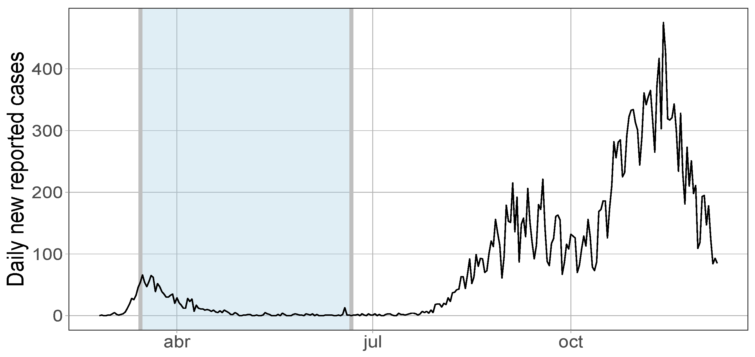
At this moment, we evaluate the hyper-parameters of the different marginal prior distributions given in (6)–(8). The population of the province of Cádiz is estimated at p = 1,240,155 inhabitants, so the value of $\alpha$ is $12.40155$. Just considering the confirmed cases per 100,000 people shown in Figure 1 for the Spanish ACs at the beginning of the pandemic and changing the scale by $\alpha$ we obtain the Maximum Likelihood Estimate (MLE) for the mean and the scale parameters in (6), i.e., $\mu =399.95$ and $\beta =525.21$, respectively. The value $M=10$ was determined because it was not found any case where the number of infections at the beginning were bigger. We would like to emphasize that in this first wave M had little informative value to obtain the posterior distribution of b as we have checked by taking different values for M and just observing the posterior expected quantity for $M_0=1.14$ and its posterior standard deviation equal to $0.15$ shown in

Table 1. Bayesian estimates of the the main parameters in the hypothetical scenario of no restrictions in the first wave in the province of Cádiz (1,240,155 inhabitants).

Param.	Post. Mean	sd	2.5% CI	50% CI	97.5% CI	${\mathit{n}}_{\mathit{e}\mathit{f}\mathit{f}}$	$\widehat{\mathit{R}}$
a	27,766.41	11,916.20	10,865.82	25,456.36	56,400.37	3221.76	1
b	10.02	0.44	9.15	10.03	10.83	3138.09	1
c	0.04	0.00	0.04	0.04	0.05	2919.79	1
$M_0$	1.14	0.15	1.00	1.09	1.53	4115.42	1
$T_{max}$	53.13	4.48	44.29	53.10	61.86	2953.03	1

. In other words, the result of the estimation is essentially independent of the choice of M in this case. Finally, to bound the values of $c_1=0.01$ and $c_2=0.2$, we take into account the highest and the lowest values found in Spain and other countries, as it is seen in [34,35,37]. Those values are also reasonable with the observed range in Figure 1 described in [33].

3.1. Forecasts for the Characteristics of Interest at Different Scenarios

In order to evaluate our model, we will estimate the functionals given in (9)–(11) at different stages of the pandemic. As a natural question, we first are interested in evaluating the benefits of the first lockdown imposed by the Spain’s central government. Second, we will locate our estimates during the lockdown and close to the end of the State of Alarm to verify not only that predictions are quite accurate, but also how daily new cases decrease. Finally, just observing the evolution of our estimates after the easing of Spain’s lockdown restrictions, we will be able to detect the beginning of the second and third waves by the increase of the daily number of new reported contagious.

3.1.1. First Scenario: The Benefits of the Lockdown

The lockdown in Spain was imposed on 14 March 2020. Therefore, in order to evaluate the benefits of that decision in the province of Cádiz, we will first consider T, the ending day, as 15 March 2020. The idea is to make daily predictions of the following week, from 16 March 2020 to 22 March 2020. Moreover, it is worth mentioning that week was close to the date of the maximum number of daily new reported cases of COVID-19 in the first wave. We are aware that the classical Gompertz curve is a poor model in the early stages of an epidemic. However one of the advantages of the Bayesian approach is the incorporation of prior information which leads to a better inference for small samples.

Figure 3a shows the observed time series of the daily cumulative cases up to T—to feed the Bayesian model—and a week after T (brown). Likewise, it shows a set of 500 Gompertz curves obtained by an i.i.d. random sample of size 500 from the posterior distribution ${\pi }_{\mathbf{x}}$ (grey). It is remarkable the band of the Gompertz curves leads us to predict the trend of daily cumulative positive cases of SARS-CoV-2 by incorporating variability. Figure 3b shows the observed time series of the daily cases up to T (black) and a week after T (brown). It also shows the expectation (blue) and the $95\%$ CI (blue dash line) of $E_{T+d}^{T+d+1}\left({\pi }_{\mathbf{x}}\right)$ as forecasts of the expected number of new daily cases of COVID-19 where $d\in \{0,\dots ,6\}$.

At first glance, a change in trend can be observed between the predictions of the expected values (which continues an upward trend) and the observed data after T, which begins a downward trend. For that reason, it seems that the lockdown imposed by the authorities was beneficial to control the initial evolution of the pandemic by reducing the daily number of expected new cases.

Regarding to the parameters of interest, it is remarkable that in case of no restrictions—no government interventions- after T, we estimate that the $95\%$ CI for the parameter a—maximum number of infected—would lie on the interval $(10,865.82,56,400.37)$ having a posterior mean of 27,766.41 inhabitants, see Table 1. As the population size in Cádiz is 1,240,155 inhabitants, no restrictions could mean that approximately the $2\%$ of population would be infected by the disease. Of course, this number could have meant the collapse of the health system and would have caused a much higher number of deaths. Additionally, the posterior mean of the time to reach the peak would have been $E^{{\pi }_{\mathbf{x}}}\left[T_{max}\left(\mathbf{\theta }\right)\right]=53.13$ days, letting the effect of the pandemic considerably would have dragged on. Fortunately it was not the case.

Results of this model can be checked in a ShinyStan App at https://micromegas.shinyapps.io/COVID-19-Scenario1-CA-province/.

3.1.2. Second Scenario: The Evolution of the Pandemic during the Lockdown

Now we will evaluate the goodness of fit of our model by making predictions during the lockdown period. For such a purpose, we will consider T, the ending day, as 3 May 2020. As in the first scenario, the idea is to make daily predictions for the following week, from 4 May 2020 to 10 May 2020. It is worth mentioning that the decrease of the number of new daily cases during the lockdown was the reason why Spanish authorities justified the end of the lockdown on 21 June 2020.

Analogously to Figure 3 and Figure 4a shows the time series of observed daily cumulative cases up to T (black) and a week after T (brown). Moreover, shows a band of Gompertz curves obtained from an i.i.d. random sample of the posterior distribution ${\pi }_{\mathbf{x}}$ (grey).

Moreover, analogously to Figure 3 and Figure 4b shows the observed time series of daily new cases (black) up to T and a week after T (brown). It also shows the forecasts of the expected number of new daily cases as the posterior mean of $E_{T+d}^{T+d+1}\left({\pi }_{\mathbf{x}}\right)$ (blue) and its $95\%$ CI (blue dash line). In addition, we also compute the $95\%$ CI of $Q_{T+d}^{T+d+1}(0.975,{\pi }_{\mathbf{x}})$ (red band) and $Q_{T+d}^{T+d+1}(0.025,{\pi }_{\mathbf{x}})$ (green band), where $a\in \{0,\dots ,6\}$. Those quantiles lead us to measure where the middle $95\%$ of the daily new cases lies.

At first glance, the trend of both daily and cumulative expected values are quite similar to the observed data which implies that our model fits reasonably well the observations.

Table 2. Bayesian estimates of the the main parameters during the lockdown in the first wave in the province of Cádiz (1,240,155 inhabitants).

Param.	Post. Mean	sd	2.5% CI	50% CI	97.5% CI	${\mathit{n}}_{\mathit{e}\mathit{f}\mathit{f}}$	$\widehat{\mathit{R}}$
a	1543.87	40.13	1465.62	1543.42	1622.46	6867.77	1
b	7.25	0.09	7.03	7.28	7.37	6590.83	1
c	0.08	0.00	0.08	0.08	0.08	6210.55	1
$M_0$	1.10	0.10	1.00	1.06	1.36	6583.56	1
$T_{max}$	24.73	0.36	24.02	24.72	25.43	7327.45	1

shows a summary of the Bayesian estimates of the main parameters. As a first conclusion, it seems the lockdown had a direct effect on the estimates compared to the values given in Table 1. Now the posterior mean of the maximum cumulative number of confirmed cases in the province of Cádiz, parameter a, is about $1543.87$ people, close to the official cumulative number of confirmed cases at the end of the State of Alarm and having a $95\%$ CI of $(1465.62,1622.46)$. Therefore, we estimate that about $0.12\%$ of the population of the province of Cádiz was detected as a confirmed case of COVID-19 in the first wave and until the end of the lockdown. Taking into account that less than one out of ten cases was detected in the first wave, as it is described in [44], our result seems consistent with seroprevalence studies made in Spain, where it was determined that $1.7\%$ of inhabitant in the province of Cádiz presented IgG antibody against SARS-CoV2. Additionally, we also estimate that $E^{{\pi }_{\mathbf{x}}}\left(T_{max}\left(\mathbf{\theta }\right)\right)=24.73$ days having a $95\%$ CI $(24.02,25.43)$. All those estimates are close to the official data provided by RENAVE which predicts the peak in 20 days from 25 February 2020. To sum up, we would like to emphasize that a direct computation shows that the effect of the lockdown reduced the number of infected cases by about $94.5\%$.

Results of this model can be checked in a ShinyStan App at https://micromegas.shinyapps.io/COVID-19-Scenario2-CA-province/.

In Spain, the end of the lockdown was on 21 June 2020 and our model fits reasonable well during that period and forecasts stop being as good after lockdown. It is apparent the easing of restrictions lead to a new change in the trend and the arrival of a new wave. We will see in the following scenario how we can predict it.

3.2. Detecting the Beginning of a New Wave

As we have mentioned, the model fits well the evolution of the number of new cases during the lockdown. By considering T, the end of the lockdown, as 21 June, we next propose a classical tool to detect the beginning of a future wave based on the $99\%$ percentile of the number of daily new cases. For such a purpose, we first estimate daily quantiles by the posterior mean of $Q_{T+d}^{T+d+1}(0.99,{\pi }_{\mathbf{x}})$, where $d\in \{0,\dots ,41\}$, i.e., for the first 42 days—6 weeks—after the lockdown. Second, for the ith week we count the cumulative number of confirmed cases where the observed daily number of contagious exceeding the estimate of the $99\%$ daily quantile, and we will denote it by $W_i^{+}$, $i=1,\dots ,6$. For example, $W_1^{+}=1$ means that just one day the observed new daily cases exceed the estimate of the $99\%$ daily quantile in the first week after the lockdown. It is apparent that $W_i^{+}$ is a risk measure that takes values from 0 to 7, $i=1,\dots ,6$, and the larger the value, the greater the probability of a new wave.

Table 3. The risk measure week-by-week to predict a new wave of COVID-19 in the province of Cádiz where the first week ranges from 22 June to 28 June and the 6 week from 27 July to 2 August.

$\mathbf{Week}$	1st	2nd	3rd	4th	5th	6th
$W_i^{+}$	2	3	3	6	7	7

shows the values of $W_i^{+}$, $i=1,\dots ,6$, in the province of Cádiz. Note the first week ranges from 22 June to 28 June and the sixth week from 27 July to 2 August. It is apparent that easing COVID-19 restrictions after the lockdown leads to more spreading of coronavirus in just a few weeks.

Again we face the problem to establish the time zero as mentioned in Remark 2. The value $W_5^{+}=7$ in Table 3 implies that in all days in the 5th week the observed new daily cases exceed the estimate of the 99% daily quantile. Therefore, in order to make predictions in the second wave we have considered the initial date as 27 July, five weeks after the lockdown was finished, and T, the ending day, as 13 September 2020. We would like to emphasize that Spain had one of the most restrictive lockdown in the world in the first wave. After the lockdown people were afraid of going back to normal. We think this was the main reason of slow growth at the beginning of July. However, little by little people in summer were more confidence and jointly to an attempt to save the tourist season, infections started growth again at the end of July. It is apparent that initial conditions in the first and second waves are different. Therefore the value of the hyper-parameter $M=100$ was determined taking into account that the initial cases of the second waves are, in some sense, determined by the cases at the end of the first wave. Finally, we consider the same prior information for the parameters a and c in order to have more prior variability.

The parameters of interest are shown in

Table 4. Bayesian estimates of the main parameters during the second wave in the province of Cádiz (1,240,155 inhabitants).

Param.	Post. Mean	sd	2.5% CI	50% CI	97.5% CI	${\mathit{n}}_{\mathit{e}\mathit{f}\mathit{f}}$	$\widehat{\mathit{R}}$
a	14,980.964	1630.937	12,335.926	14,791.462	18,628.804	1332.199	1.002
b	5.746	0.116	5.523	5.745	5.975	3338.672	1.000
c	0.032	0.002	0.028	0.032	0.035	1304.779	1.002
$M_0$	48.342	8.654	33.606	47.567	67.095	1550.593	1.001
$T_{max}$	55.179	3.037	49.978	54.926	61.736	1318.682	1.002

. Note the second wave can be interpreted as an intermediate scenario between having no restrictions and the lockdown. Now the posterior mean of the maximum number of infected in the province of Cádiz, a, is about 14,980.964 people and we also estimate that $E^{{\pi }_{\mathbf{x}}}\left(T_{max}\left(\mathbf{\theta }\right)\right)=55.179$. We recall that differences between the first and second wave can be attributed to both a higher rate of contagious and an increase of the number of people tested as described in Remark 4.

As a complementary study, Andalusia is divided into eight provinces, namely Almeria, Granada, Jaén, Málaga, Sevilla, Córdoba, Cádiz and Huelva. We compute the evolution of the risk measure given in Table 3 for all of them. In order to make predictions, we only should take in account they have different population size, i.e., different $\alpha$ = P/100,000 in Expression (6).

Table 5. Population size of the eight provinces of Andalusia.

Prov.	Almería	Cádiz	Córdoba	Granada	Huelva	Jaén	Málaga	Sevilla
P	716,820	1,240,155	782,979	914,678	521,870	633,564	1,661,785	1,942,389

shows the population sizes, P, of the eight Andalusian provinces (population size according to the Instituto Nacional de Estadística https://www.ine.es/up/9Gq4uzeUiT).

Figure 5 shows the evolution of the risk measure in Andalusia by using a color map. This figures allows us to make inter-provincial comparisons and detect how the effects of COVID-19 vary between provinces and territories.

To conclude our analysis, we have studied the evolution of the confirmed cases in the province of Cádiz during the autumn period. We first fix the beginning of the second wave as 27 July and T as 20 September. By using a similar argument as in the detection of the second wave, we compute the measure $W_i^{+}$ for the following four weeks, $i=1,2,3$ and 4, obtaining 3, 3, 4 and 6, respectively. It seems a third wave appears in the fourth week from the beginning of the second wave. In addition, that fourth week coincides with a vacation period in Spain. Therefore, we finally establish the beginning of the third wave as 11 October. In contrast to the second wave, the third wave appears before flattening the second curve.

By using data from 11 October to 8 December 2020—the submission date of this work—we present in

Table 6. Bayesian estimates of the main parameters during the third wave in the province of Cádiz (1240155 inhabitants).

Param.	Post. Mean	sd	2.5% CI	50% CI	97.5% CI	${\mathit{n}}_{\mathit{e}\mathit{f}\mathit{f}}$	$\widehat{\mathit{R}}$
a	18,009.32	200.45	17,622.73	18,007.82	18,416.35	3327.78	1
b	3.76	0.06	3.63	3.76	3.89	3210.05	1
c	0.052	0.001	0.050	0.052	0.053	2791.33	1
$M_0$	418.81	29.54	363.10	418.00	481.48	2889.03	1
$T_{max}$	25.54	0.23	25.08	25.54	26.01	8387.82	1

the parameters of interest of the third wave. Again the hyper-parameter $M=1000$ has been modified because the third wave started having higher initial values at time zero.

Finally, we present in Figure 6 the band of Gompertz curve for the second wave (green) and the band of Gompertz curve for the third wave (orange) obtained from an i.i.d. random sample of the posterior distributions. It is apparent that models fit well data. From the interpretation of $1/c$ as the width (duration) of a wave and just observing the estimates of the parameter c in Table 2, Table 4 and Table 6, it is apparent that the duration of the second wave (if it were not interrupted by the third) would be more than twice longer that the duration of the first one and the third wave seems to be a bit shorter than the second one.

4. Conclusions

We have presented a non-homogeneuos Poisson process with intensity function based on the classical Gompertz curve for modeling and forecasting COVID-19 pandemic by using Bayesian inference. In that context, we have discussed the prior distributions of the parameters. In particular, we propose a right-skewed distribution as the baseline prior distribution to model confirmed cases per day per 100,000 inhabitants. The inverse Gaussian distribution seems reasonable for such a purpose in Spain. The presented framework can be used for both estimating the number of individuals infected and evaluating the success of different policies. Independently of the comparison of our model to other ones, the Bayesian approach always suppose an improvement in the estimates when just small samples are available.

Clearly inspired in Risk Theory and jointly to the well-known properties of the non-homogeneuos Poisson process we propose an indicator which helps us to identify the beginning of a new wave. That indicator is based on the estimates of the 99% percentile of the number of daily new cases. To sum up, after fixing a model up to time T, we evaluate the estimates of the new confirmed cases for the following weeks and we are able to detect if real cases exceed certain threshold given by the quantiles which is the key to establish a new wave. We would like to emphasize that our model is not able to predict the onset of a new wave but at least is able to detect it. For such predictions we refer the reader to dynamical models that incorporate mechanisms of social response, such as attempted in [45].

To conclude, applying our method to the province of Cádiz, located at the South of Spain, we were able to discuss the effectiveness of the first lockdown, the accuracy of the estimates during that lockdown and the beginning of the second and third waves after the lockdown. For future works it would be interesting to apply robust Bayesian techniques as described in [46,47,48,49]. In particular, it would be interesting to consider a band of prior distributions for the parameter a as described in [46]. Additionally, the relative range of variation of a is larger than for c where further research is needed to find causal mechanism to interpret those ranges. Finally, it is worth mentioning that the hyper-parameter M—which induces uncertainty in the initial cases—takes different values depending on the wave. For example, it is apparent that the initial cases in the first, second and third waves were different.

References

1. Lu, R.; Zhao, X.; Li, J.; Niu, P.; Yang, B.; Wu, H.; Wang, W.; Song, H.; Huang, B.; Zhu, N.; et al. Genomic characterisation and epidemiology of 2019 novel coronavirus: Implications for virus origins and receptor binding. Lancet 2020, 395, 565–574. [Google Scholar] [CrossRef] [Green Version]
2. Bolsen, T.; Palm, R.; Kingsland, J. Framing the Origins of COVID-19. Sci. Commun. 2020, 42, 562–585. [Google Scholar] [CrossRef]
3. Kermack, W.; McKendrick, A. Contributions to the Mathematical Theory of Epidemics. Proc. R. Soc. A 1927, 115, 700–721. [Google Scholar]
4. Becker, N.; Britton, T. Statistical studies of infectious disease incidence. J. R. Stat. Soc. B 1999, 61, 287–307. [Google Scholar] [CrossRef]
5. O’Neill, P. A tutorial introduction to Bayesian inference for stochastic epidemic models using Markov chain Monte Carlo methods. Math. Biosci. 2002, 180, 103–114. [Google Scholar] [CrossRef]
6. Grassly, N.; Fraser, C. Mathematical models of infectious disease transmission. Nat. Rev. Microbiol. 2008, 6, 477–487. [Google Scholar] [CrossRef]
7. Krämer, A.; Kretzschmar, M.; Krickeberg, K. Modern Infectious Disease Epidemiology Concepts, Methods, Mathematical Models and Public Health; Springer: New York, NY, USA, 2010. [Google Scholar]
8. Brauer, F.; Driessche, P.V.D.; Wu, J. Mathematical Epidemiology; Springer: New York, NY, USA, 2000. [Google Scholar]
9. Clayton, D.; Hills, M. Statistical Models in Epidemiology; Oxford University Press: Oxford, UK, 2013. [Google Scholar]
10. Keeling, M.; Rohani, P. Modeling Infectious Diseases in Humans and Animals; Princeton University Press: Princeton, NJ, USA, 2007. [Google Scholar]
11. Thompson, W.; Comanor, L.; Shay, D. Epidemiology of seasonal influenza: Use of surveillance data and statistical models to estimate the burden of disease. J. Infect. Dis. 2006, 194, S82–S91. [Google Scholar] [CrossRef] [Green Version]
12. Fineberg, H.; Wilson, M. Epidemic science in real time. Science 2009, 324, 987. [Google Scholar] [CrossRef] [Green Version]
13. Pell, B.; Kuang, Y.; Viboud, C.; Chowell, G. Using phenomenological models for forecasting the 2015 Ebola challenge. Epidemics 2018, 22, 62–70. [Google Scholar] [CrossRef] [Green Version]
14. Berger, J.O. Statistical Decision Theory and Bayesian Analysis, 2nd ed.; Springer: New York, NY, USA, 1985. [Google Scholar]
15. Ríos Insua, D.; Ruggeri, F. Robust Bayesian Analysis; Lecture Notes in Statistics 152; Springer: New York, NY, USA, 2000. [Google Scholar]
16. Bernardo, J.M. Bayesian Statitistics; Viertl, R., Ed.; Encyclopedia of Life Support Systems (EOLSS), Probability and Statistics; UNESCO: Oxford, UK, 2003. [Google Scholar]
17. Flaxman, S.; Mishra, S.; Gandy, A.; Unwin, H.; Coupland, H.; Mellan, T.; Zhu, H.; Berah, T.; Eaton, J.W.; Guzman, P.; et al. Estimating the number of infections and the impact of non-pharmaceutical interventions on COVID-19 in 11 European countries. Imp. Coll. Lond. 2020. [Google Scholar] [CrossRef]
18. Jha, P.; Cao, L.; Oden, J. Bayesian-based predictions of COVID-19 evolution in Texas using multispecies mixture-theoretic continuum models. Comput. Mech. 2020. [Google Scholar] [CrossRef] [PubMed]
19. Manevski, D.; Gorenjec, N.R.; Kejžar, N.; Blagus, R. Modeling COVID-19 pandemic using Bayesian analysis with application to Slovene data. Math. Biosci. 2020, 329. [Google Scholar] [CrossRef] [PubMed]
20. Emery, J.; Russell, T.; Liu, Y.; Hellewell, J.; Pearson, C.; CMMID COVID-19 Working Group; Knight, G.; Eggo, R.; Kucharski, A.; Funk, S.F.; et al. The contribution of asymptomatic SARS- CoV-2 infections to transmission on the Diamond Princess cruise ship. eLife 2020. [Google Scholar] [CrossRef]
21. Lee, S.; Lei, B.; Mallick, B. Estimation of COVID-19 spread curves integrating global data and borrowing information. PLoS ONE 2020, 7. [Google Scholar] [CrossRef]
22. Kingman, J. Poisson Processes; Clarendon Press: Oxford, UK, 1993. [Google Scholar]
23. Ríos Insua, D.; Ruggeri, F.; Wiper, M. Bayesian Analysis of Stochastic Process Models; Wiley: New York, NY, USA, 2012. [Google Scholar]
24. McCollin, C. Intensity Functions for Nonhomogeneous Poisson Processes; Wiley StatsRef: Statistics Reference Online; John Wiley & Sons, Ltd.: Hoboken, NJ, USA, 2014. [Google Scholar]
25. Gompertz, B. Xxiv. On the nature of the function expressive of the law of human mortality, and on a new mode of determining the value of life contingencies. in a letter to francis baily, esq. frs &c. R Package Version 1825, 2, 513–583. [Google Scholar]
26. Madden, L. Quantification of disease progression. Prot. Ecol. 1980, 2, 159–176. [Google Scholar]
27. Zwietering, M.; Jongenburger, I.; Rombouts, F.; Riet, K.V. Modeling of the bacterial growth curve. Appl. Environ. Microbiol. 1990, 56, 1875–1881. [Google Scholar] [CrossRef] [Green Version]
28. Berger, R. Comparison of the Gompertz and Logistic Equations to describe plant disease progress. Phytopathology 1981, 71, 716–719. [Google Scholar] [CrossRef]
29. Löytönen, M. The Spatial Diffusion of Human Immunodeficiency Virus Type 1 in Finland, 1982–1997. Ann. Assoc. Am. Geogr. 1991, 81, 127–151. [Google Scholar] [CrossRef]
30. Alonso-Prados, L.; Luis-Arteaga, J.; Alvarez, M.; Moriones, E.; Batlle, A.; Laviña, A.; García-Arenal, F.; Fraile, A. Epidemics of Aphid-transmitted Viruses in Melon Crops in Spain. Eur. J. Plant Pathol. 2003, 109, 129–138. [Google Scholar] [CrossRef]
31. Yang, Z.; Jiao, X.; Li, P.; Pan, Z.; Huang, J.; Gu, R.; Fang, W.; Chao, G. Predictive model of Vibrio parahaemolyticus growth and survival on salmon meat as a function of temperature. Food Microbiol. 2009, 26, 606–614. [Google Scholar] [CrossRef] [PubMed]
32. Jenner, A.L.; Kim, P.; Frascoli, F. Oncolytic virotherapy for tumours following a Gompertz growth law. J. Theor. Biol. 2019, 480, 129–140. [Google Scholar] [CrossRef] [PubMed]
33. Rypdal, K.; Rypdal, M. A Parsimonious Description and Cross-Country Analysis of COVID-19 Epidemic Curves. Int. J. Environ. Res. Public Health 2020, 18, 6487. [Google Scholar] [CrossRef] [PubMed]
34. Díaz-Pérez, F.; Chinarro, D.; Pino-Otin, R.; Díaz-Martín, R.; Díaz, M.; Guardiola-Mouhaffel, A. Comparison of Growth Patterns of COVID-19 Cases through the ARIMA and Gompertz Models. Case Studies: Austria, Switzerland, and Israel. Rambam Maimonides Med. J. 2020, 11, 1–13. [Google Scholar] [CrossRef]
35. Díaz-Pérez, F.; Chinarro, D.; Pino-Otin, R.; Guardiola-Mouhaffel, A. Growth forecast of the COVID-19 with the Gompertz function, Case study: Italy, Spain, Hubei, China. Int. J. Adv. Eng. Res. Sci. 2020, 7, 67–77. [Google Scholar] [CrossRef]
36. Medina-Mendieta, J.; Cortés-Cortés, M.; Cortés-Iglesias, M. COVID-19 Forecasts for Cuba Using Logistic Regression and Gompertz Curves. MEDICC Rev. 2020, 22, 32–39. [Google Scholar]
37. Ohnishi, A.; Namekawa, Y.; Fukui, T. Universality in COVID-19 spread in view of the Gompertz function. Prog. Theor. Exp. Phys. 2020. [Google Scholar] [CrossRef]
38. Sánchez-Villegas, P.; Colina, A. Modelos predictivos de la epidemia de COVID-19 en España con curvas de Gompertz. Gac. Sanit. 2020. [Google Scholar] [CrossRef]
39. Asadi, M.; Di Crescenzo, A.; Sajadi, F.A.; Spina, S. A generalized Gompertz growth model with applications and related birth-death processes. Ric. Mat. 2020, 1–36. [Google Scholar] [CrossRef]
40. Hoffman, M.D.; Gelman, A. The No-U-Turn sampler: Adaptively setting path lengths in Hamiltonian Monte Carlo. J. Mach. Learn. Res. 2014, 15, 1593–1623. [Google Scholar]
41. Carpenter, B.; Gelman, A.; Hoffman, M.D.; Lee, D.; Goodrich, B.; Betancourt, M.; Brubaker, M.; Guo, J.; Li, P.; Riddell, A. Stan: A Probabilistic Programming Language. J. Stat. Softw. 2017, 76. [Google Scholar] [CrossRef] [Green Version]
42. Stan Development Team. RStan: The R Interface to Stan, R Package Version 2.19.3. Available online: https://mc-stan.org/users/interfaces/rstan.html (accessed on 14 April 2020).
43. Gabry, J. Shinystan: Interactive visual and numerical diagnostics and posterior analysis for bayesian models. Philos. Trans. R. Soc. Lond. 2015, 115. Available online: https://mc-stan.org/users/interfaces/shinystan (accessed on 14 April 2020).
44. Pullano, G.; Domenico, L.D.; Sabbatini, C.; Valdano, E.; Turbelin, C.; Debin, M.; Guerrisi, C.; Kengne-Kuetche, C.; Souty, C.; Hanslik, T.; et al. Underdetection of cases of COVID-19 in France threatens epidemic control. Nature 2020. [Google Scholar] [CrossRef] [PubMed]
45. Dolbeault, J.; Turinici, G. Social heterogeneity and the COVID-19 lockdown in a multi-group SEIR model. medRxiv 2020. [Google Scholar] [CrossRef]
46. Arias-Nicolás, J.; Ruggeri, F.; Suárez-Llorens, A. New Classes of Priors Based on Stochastic Orders and Distortion Functions. Bayesian Anal. 2016, 11, 1107–1136. [Google Scholar] [CrossRef]
47. Barrera, M.; Lira, I.; Sánchez-Sánchez, M.; Suárez-Llorens, A. Bayesian treatment of results from radioanalytical measurements. Effect of prior information modification in the final value of the activity. Radiat. Phys. Chem. 2019, 156, 266–271. [Google Scholar] [CrossRef]
48. Sánchez-Sánchez, M.; Sordo, M.A.; Suárez-Llorens, A.; Gómez-Déniz, E. Deriving Robust Bayesian Premiums under Bands of Prior Distributions with Applications. ASTIN Bull. 2019, 49, 147–168. [Google Scholar] [CrossRef]
49. Ruggeri, F.; Sánchez-Sánchez, M.; Sordo, M.; Suárez-Llorens, A. On a New Class of Multivariate Prior Distributions: Theory and Application in Reliability. Bayesian Anal. Adv. Publ. 2020. [Google Scholar] [CrossRef]
Figure 1. Goodness of fit new confirmed cases per day per 100,000 people, April 2020.
Mathematics 09 00228 g001
Figure 2. Time series of the daily new reported cases of COVID-19 in the province of Cádiz. Blue color shows the period of the State of Alarm in Spain from 14 March to 21 June 2020.
Mathematics 09 00228 g002
Figure 3. (a) Time series of observed daily cumulative cases up to T (black) and a week after T (brown). A band of Gompertz curves given by an i.i.d. random sample of size 500 of g ( t π x ) (grey). (b) Time series of observed daily cases up to T (black) and a week after T (brown). The expectation (blue) and the 95 % CI (blue dash line) of E T + d T + d + 1 ( π x ) , d { 0 , , 6 } .
Mathematics 09 00228 g003
Figure 4. (a) Time series of observed daily cumulative cases up to T (black) and a week after T (brown). A band of Gompertz curves given by an i.i.d. random sample of size 500 of g ( t π x ) (grey). (b) Time series of observed daily cases up to T (black) and a week after T (brown). The expectation (blue) and the 95 % CI (blue dash line) of E T + d T + d + 1 ( π x ) , d { 0 , , 6 } . The 95 % CI of Q T + d T + d + 1 ( 0.975 , π x ) (red band) and Q T + d T + d + 1 ( 0.025 , π x ) (green band), where d { 0 , , 6 } .
Mathematics 09 00228 g004
Figure 5. Evolution of the beginning of the second wave after the ending of the Lockdown in the eight provinces of Andalusia.
Mathematics 09 00228 g005
Figure 6. Time series of observed daily cumulative cases from 27 July to 8 December (black). The Gompertz curves band for the second wave (green) and the Gomperts curves band for the third wave (orange), given by an i.i.d. random sample of size 500 of g ( t π x ) of the respective posterior distributions.
Mathematics 09 00228 g006