Volatility Forecasting for High-Frequency Financial Data Based on Web Search Index and Deep Learning Model

Abstract

The existing index system for volatility forecasting only focuses on asset return series or historical volatility, and the prediction model cannot effectively describe the highly complex and nonlinear characteristics of the stock market. In this study, we construct an investor attention factor through a Baidu search index of antecedent keywords, and then combine other trading information such as the trading volume, trend indicator, quote change rate, etc., as input indicators, and finally employ the deep learning model via temporal convolutional networks (TCN) to forecast the volatility under high-frequency financial data. We found that the prediction accuracy of the TCN model with investor attention is better than those of the TCN model without investor attention, the traditional econometric model as the generalized autoregressive conditional heteroscedasticity (GARCH), the heterogeneous autoregressive model of realized volatility (HAR-RV), autoregressive fractionally integrated moving average (ARFIMA) models, and the long short-term memory (LSTM) model with investor attention. Compared with the traditional econometric models, the multi-step prediction results for the TCN model remain robust. Our findings provide a more accurate and robust method for volatility forecasting for big data and enrich the index system of volatility forecasting.

1. Introduction

The volatility of financial asset prices is one core factor for risk measurement, financial derivatives pricing, and asset allocation. Accurate volatility forecasting has become one of the hot topics in academic and industry research. Considering the volatility aggregation of the asset returns, Engle [1] introduced the autoregressive conditional heteroskedasticity model (ARCH) model for the residual series. Later, Bollerslev [2] proposed the generalized autoregressive conditional heteroscedasticity (GARCH) model to fully describe the volatility process of the asset return. Baillie et al. [3] used the integral autoregressive conditional heteroscedasticity model (FIGARCH) model to reflect the heteroscedasticity characteristics of financial assets and the variation characteristics of long memory. Taylor [4] proposed the stochastic volatility (SV) model based on the condition that the conditional variance followed an unobservable stochastic process, and used low-frequency data to measure the daily volatility. The aforementioned models for volatility modeling are mainly based on low-frequency data such as daily or monthly asset returns. With the innovation and development of big data technology, the storage capacity and computing power of high-frequency financial time series have been significantly improved. Computational modeling and forecasting analysis based on high-frequency financial time series have become important research topics for scholars. Andersen and Bollerslev [5] firstly proposed that the sum of squares of intraday high-frequency returns should be used to calculate intraday volatility. Corsi [6] and Anderson et al. [7] used the heterogeneous autoregressive model of realized volatility (HAR-RV) model and autoregressive fractionally integrated moving average (ARFIMA) model to forecast the volatility based on the realized volatility calculated by intraday high-frequency financial data, and found that the models had better out-of-sample volatility forecasting than the traditional GARCH family models.

The volatility of index price is also affected by economic factors, policy influence, and investor attention. The mechanism of these influencing factors is usually nonlinear. On the one hand, the above-mentioned traditional econometric models only describe the dependence of volatility based on the form of the quadratic function, and could not effectively characterize the highly complex and nonlinear characteristics of the stock market; on the other hand, they only used a single index such as asset return series or historical volatility to characterize and forecast the volatility and did not take into account factors such as other transaction information and investor attention. The deep learning models can provide new ideas for improving prediction accuracy based on their fitting of nonlinear relationships and strong data feature learning capabilities. Jiang et al. [8] used the deep learning models, long short-term memory (LSTM) and recurrent neural network (RNN), to forecast stock prices respectively, and found that the LSTM model, which could describe the memory of time series, was more effective. Jin et al. [9] introduced investor attention tendencies into LSTM to predict stock closing prices. Deng et al. [10] found that the deep learning model temporal convolutional networks (TCN) could forecast the stock prices with higher accuracy. At present, deep learning models are mostly used in forecasting stock prices. However, volatility forecasting under high-frequency data is relatively rare based on the deep learning models, especially the TCN model, which has a better forecasting effect and is worthy of in-depth application research.

Other trading information such as trading volume, trend indicators, quote change rate, and other indicators were verified in our study to possess a certain correlation with volatility, and should be included as the input indicators for volatility forecasting. In addition, the Baidu search index is based on the daily behavior data of massive netizens, which reflects the “user attention” and “media attention” in the past period. It can be used as a proxy variable for investor attention. Yang and Lv [11] quantified investor attention based on the Baidu search index and explained the stock market fluctuations through emergency attention. Chen et al. [12] selected the Baidu search index and others as an online public opinion indicator for the changes in investor attention, and regressed and analyzed the relationship between investor attention and stock price index. Investors make decisions based on various information released by experts, scholars, and government agencies, and reflect their current and future information expectations of the stock market during the exchange process. In the era of the Internet economy, the web search index disclosed by Baidu can reflect investor attention. An empirical analysis of the Baidu index and stock price index shows that Baidu index is related to stock price index and can predict stock price. To avoid having too many keywords for the Baidu search index, we selected and synthesized an initial keyword library based on the screening method in Zhang and Zhou [13] and the analysis method in Li and Fan [14]. Then, we used the time-difference correlation analysis method to select the search indexes of certain specific keywords as the antecedent keywords for the volatility of the Shanghai Stock Exchange Index, which were used as the input indicator for volatility forecasting.

Under the five-minute high-frequency financial transaction data of the Shanghai Stock Exchange Index, we not only used the realized volatility as the input variable for the deep learning TCN model, but also considered other transaction information, such as transaction volume, trend indicator, quote change rate, etc., and the investor attention as the predictors for volatility forecasting. Then, we forecast the realized volatility and compared it with the traditional econometric GARCH family model, and HAR-RV, ARFIMA, and TCN models without investor attention, and the LSTM model with investor attention. The contributions of our study are twofold. Firstly, under high-frequency financial data, we took advantage of the deep learning TCN model to forecast volatility, which provided ideas for volatility forecasting in the context of big data, and enriched volatility forecasting methods. Secondly, we comprehensively sorted out the index system for volatility forecasting, especially the investor attention constructed by the Baidu search index using some antecedent keywords, which improved the accuracy of volatility forecasting.

The structure of the paper is as follows. Section 2 introduces the principle of deep learning model TCN, the research procedures, and related evaluation criteria. Section 3 uses the Baidu search index of antecedent keywords to construct the investor attention, demonstrates the correlations among other transaction information, investor attention, and the realized volatility under high-frequency data, and then selects the relevant hyperparameter of the TCN model. Finally, the accuracy and ranking of the one-step and multi-step out-of-sample volatility forecasting of nine models under five loss functions are compared. The validity of the findings that the investor attention factor through the Baidu search index positively impacts the accuracy of volatility forecasting is discussed under different calculation methods of correlation coefficient in Section 4. Section 5 concludes and extends.

2. Methods and Empirical Procedure

2.1. TCN Model

In deep learning algorithms, the modeling time series is mainly based on a recurrent neural network (RNN), while convolutional neural networks (CNN), as in LeCun et al. [15] and its extensions, are widely used in image classification tasks. After comparing the convolutional architecture and loop structure of series modeling, Bai et al. [16] found that the convolutional network performed better than the recurrent neural network in different classification and regression tasks. TCN has changed to better capture the long-distance dependence of the series forecasting model based on CNN. TCN replaces the fully connected layer with a convolutional layer to ensure that the input and output dimensions are the same. Its convolutional layer includes causal convolution and dilated convolution.

Considering that the forecasting task for time series is different from the image classification task, and the forecasting output of time series is affected by the order of the data, we should use causal convolution. The principle of causal convolution is that “we cannot know future information,” which means that the output at time t + 1 is only determined by the information at time t and before. The formulas are as follows:

$$F=\left(f_1,f_2,\dots ,f_k\right),$$

(1)

$$X=\left(x_1,x_2,\dots ,x_n\right),$$

(2)

where F represents a filter, X, as the input to the model, represents a time series, and the causal convolution at $x_t$ in the series is:

$$\left(F\ast X\right)\left(x_t\right)={\displaystyle \sum }_{k=1}^K{f}_k{x}_{t-K+k}.$$

(3)

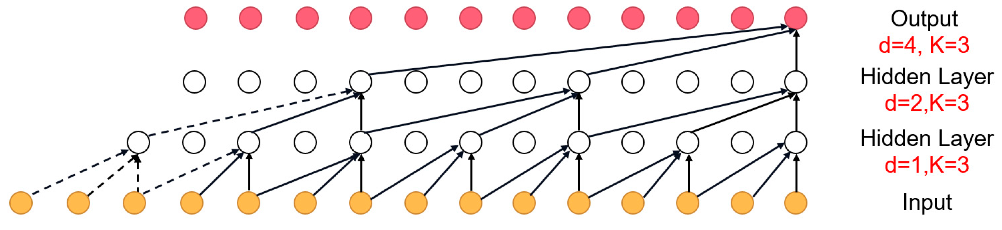
However, when processing the long history information, the number of convolutional layers of causal convolution increases, or the filter grows larger and larger to expand the receptive field. The high complexity of the model causes a vanishing gradient, thus affecting the calculation results of the model. In order to solve the problem caused by causal convolution, we used dilated convolution, which can flexibly adjust the receptive field. Dilated convolution can be regarded as a sparse process for the convolution kernel, which could make the fixed-size filter act on a wider area by skipping part of the input to obtain more information. As a result, the entire TCN model has a stable gradient, as shown in Figure 1, which is a one-dimensional 1 × 3 convolution. The dilated causal convolution at $x_t$ in the time series is:

$$\left(F{\ast }_{d}X\right)\left({\mathrm{x}}_t\right)={\sum }_{k=1}^k{f}_k{x}_{t-\left(K-k\right)\ast d},$$

(4)

where d is the dilation rate and k is the size of the convolution kernel. The receptive field can cover all values from the input sequence. Increasing d can expand the receptive field.

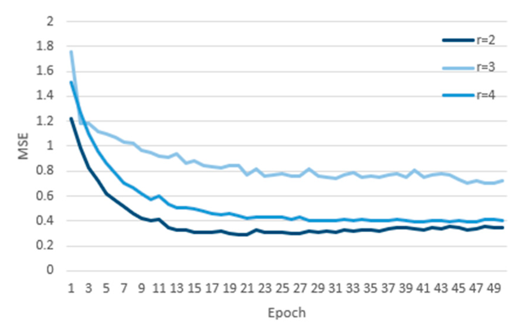
The receptive field of the model can be increased in two ways: selecting a larger filter size k and increasing the expansion factor d. The r represents the multiple of the dilation rate of each layer. For example, r = 2 represents dilation rates = [1,2,4]. TCN models with dilation rates of r = 2, r = 3, and r = 4 are constructed, and the experimental data are substituted into the model for calculation, while the loss curves are drawn by using the mean square error (MSE), as shown in Figure 2. We found that the MSE value of the TCN model with dilation rate r = 2 is the minimum under the same iteration number. Therefore, we used the TCN model with r = 2 for forecasting.

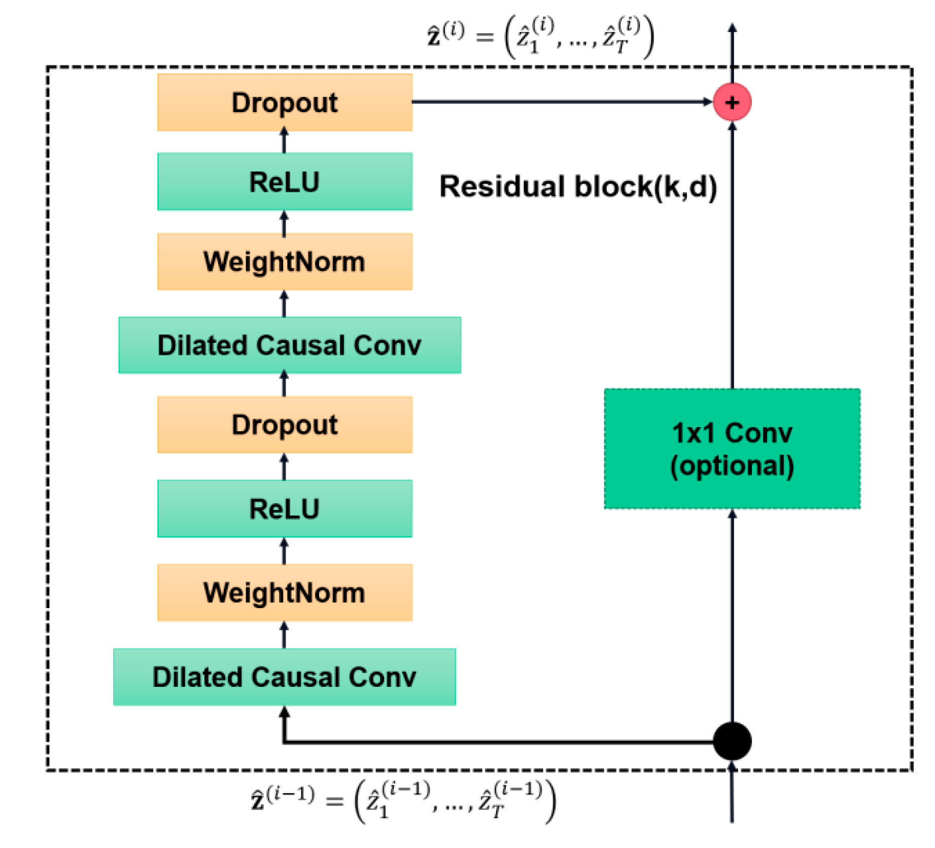
In order to prevent the dimensionality of the data from changing during the input processing, the connection method of the network we used is the residual module connection, which can make the information jump-delivery across the layer in the network. The transformation function of the ordinary connection is H(x), while the transformation function of the residual block is F(x) = H(x) − x, which only needs to learn to modify part of the input x, instead of all input x. It has great significance in solving the problem of vanishing and exploding gradients in deep networks. TCN contains two layers of causal convolution and nonlinear mapping, using rectified linear unit (ReLU) as the activation function, and adding WeightNorm and Dropout for regularization. The structure is shown in Figure 3.

In the current research, the forecasting ability of LSTM is limited by its serial calculation and large memory for training, and it does not completely solve the problem of gradient disappearance. Its derived model is not significantly improved as compared to traditional LSTM. Compared with LSTM, the parallelism of TCN can improve the computational efficiency of the model because of its identical convolution kernel. TCN uses residual block connections for causal convolutions with dilation rates. While maintaining the memory of long historical information in the series, it also completely solves the problem of gradient disappearance in the deep network; thus, TCN has a better calculation result. In summary, the TCN improves learning efficiency and optimizes the learning result, which makes it more powerful than the LSTM.

2.2. Evaluation Criteria

In our study, we used five loss functions to measure the forecasting results for each model in order to measure the accuracy of the forecasting results in multiple ways. The measurements are the mean absolute error (MAE), mean square error (MSE), root mean square error (RMSE), mean squared logarithmic error (MSLE), and mean absolute percentage error (MAPE) functions, respectively, and their specific formulas are as follows:

$$\mathrm{MAE}=\frac{1}{\mathrm{n}}\sum \left|Y-Y_{\mathrm{predict}}\right|,$$

(5)

$$\mathrm{MSE}=\frac{1}{n}\sum {\left(Y-Y_{\mathrm{predict}}\right)}^2,$$

(6)

$$\mathrm{RMSE}=\sqrt{\frac{1}{\mathrm{n}}\sum {\left(Y-Y_{\mathrm{predict}}\right)}^2},$$

(7)

$$\mathrm{MSLE}=\frac{1}{\mathrm{n}}\sum {\left(\ln \left(1+Y\right)-\ln \left(1+Y_{\mathrm{predict}}\right)\right)}^2,$$

(8)

$$\mathrm{MAPE}=\frac{100}{n}\sum _{i=1}^n\left|\frac{Y_{predict}-Y}{Y}\right|,$$

(9)

where Y represents the true value and $Y_{predict}$ denotes the forecasting value.

2.3. Empirical Procedures

The first step was the synthesis of the investor attention factor. The Baidu search index was acquired through the crawler, and then, the antecedent keywords were filtered through the time-difference correlation analysis. Finally, the investor attention factor was synthesized according to the time difference correlation coefficient between the antecedent keywords and the realized volatility.

The second step was to calculate the daily realized volatility based on the five minutes high-frequency data of the Shanghai securities composite index.

The third step was to establish the indicator system and build a TCN model to forecast the volatility. The hyperparameter of the TCN model was selected for future volatility forecasting according to the data feature.

The fourth step was the evaluation and the comparison for the forecasting models. To evaluate and compare the out-of-sample forecasting of the TCN model, the LSTM model, the GARCH family of traditional econometric models, the ARFIMA model, and the HAR-RV model, five kinds of evaluation criteria were used, which are MSE, RMSE, MAE, MAPE, and MSLE. The prediction accuracy of the deep learning model before and after adding the investor attention factor should be compared as well.

3. Empirical Results

3.1. Realized Volatility

The realized volatility was calculated as in Anderson and Bollerslev [7] and the method of calculating the true value of volatility using realized volatility as the observed volatility was based on Chen [17]. The two adjacent five-minute logarithms of closing prices $P_{t,d}$ were used to calculate the high-frequency yield rate $R_{t,d}$, which is defined as follows:

$${\mathrm{R}}_{t,d}=100\left(\ln P_{t,d}-\ln P_{t,d-1}\right),$$

(10)

where t represents the trading day, t = 1,2,3, …, 2403, $P_{t,0}$ refers to the opening price of 9:30 on the t trading day, and $P_{t,d}$ is the closing price of every five minutes on the t trading day, d = 1,2, …, 48. The realized volatility $R{V}_t$ of the day t represents the sum of the squares of all high-frequency yield rates of the day:

$$R{V}_t=\sum _{d=1}^{48}{R}_{t,d}^2.$$

(11)

3.2. Construction of Investor Attention Factor

Similar to Google search data, the Baidu index is the number of searches for a certain keyword in the Baidu search engine in a certain period, which is a free and massive data analysis service to reflect the “user attention” and “media attention” in the past. Through the Baidu index, we can mine and discover the most valuable information on the Internet, which can directly and objectively reflect the real-time hot information that netizens are interested in. The stock search data based on the Baidu index contains the interests and attentions of Chinese investors. Miao [18] used the Baidu Index to analyze 148 A-share companies, and Wang [19] used the Baidu Index to perform a regression analysis on individual stocks in Shenzhen, which showed that the Baidu index could reflect investor attention. The Baidu search index is based on the daily search volume of Baidu netizens, and, taking keywords as the statistical object, scientifically analyzes and calculates the weighted sum of search frequency of each keyword in Baidu search. The index is updated every day and the mobile wireless search index has been available since January 2011. It is described in Figure 4.

3.2.1. Acquisition of the Baidu Index

One can open the Baidu Index web page (http://index.baidu.com (accessed on 4 January 2021)), enter the keywords in the search bar, and click the query to get the daily search value of the keywords. Based on the screening method in Zhang and Zhou [13] and the analysis method in Li and Fan [14] for the keywords of the Baidu index, we synthesized the initial keyword database for our research purpose, which is shown in

Table 1. Initial keyword library.

Financial Investment	Travel	Car	Mortgage Loan
Consumption	Commerce	Credit Card	Bankruptcy
Real Estate	Industry	Advertising	Inflation
Education	Aviation	Cell Phone	Financial Crisis
Job	Computer	Small and Medium-sized Enterprises	Luxury
Insurance	Transaction	Lease	Derivative
Shopping	E-Commerce

. We used Python code to capture the daily search data from 4 January 2011 to 21 November 2020, and obtained a total of 86,712 datapoints. After excluding non-trading data, we obtained 2403 valid datapoints for each keyword. The reason for choosing “Education” is that, due to the recent COVID-19 pandemic, the education field has been hit hard, and some emerging education modes are impacting the traditional education industry. Additionally, the “Car,” “Aviation,” and “Computer” keywords represent the real economy, and the financial market relies on the real economy, which is the main factor that affects the attention of investors. Hence, we selected some keywords to be used as examples for the real economy.

3.2.2. Screening of the Baidu Search Index

Time-difference correlation analysis is a common method to use correlation coefficients to verify the antecedent, consistent, or lagging relationship of economic time series. The calculation procedure is as follows. After selecting appropriate benchmark indicators that can sensitively and accurately reflect economic performance, one moves the selected indicators forward or backward in time for several days, and then calculates the correlation coefficients between the benchmark indicators and these shifted sequences. After this movement, according to the positive and negative order of time delay, the antecedent indicators leading to the changes in the benchmark indicators, the consistent indicators that are basically the same as the changes in the benchmark indicators, and the lagging indicators that lag behind the changes in the benchmark indicators are selected. When the time difference correlation coefficient reaches the maximum value, the delay coefficient is the corresponding number of antecedent or lag periods. We calculated the correlation between the Baidu search index of each keyword and the volatility of the Shanghai Composite Index based on time-difference correlation analysis and verified the forward–backward correlation and lead–lag relationship of indexes. Keywords can be divided into three categories according to the time difference relationship: antecedent keywords, which have a trend ahead of the Shanghai Composite Index; consistent keywords, which are basically consistent with the Shanghai Composite Index on the trend; and lagging keywords, which lag behind the trend of Shanghai Composite Index. Selecting the antecedent keywords for forecasting can reduce the number of parameters and improve the forecasting accuracy. The filtering method of search keywords is as follows.

The first step was to determine the benchmark index and analysis index. The benchmark index series is the variable to be predicted. In this study, the predicted variable is the daily volatility of the Shanghai Composite Index, and the 24 keywords series from Baidu Search Index is used as the analysis index series.

The second step was to calculate the correlation coefficient as well as the time delay order of the analysis index series and the benchmark index series according to the formula of the time difference correlation analysis as follows:

$$r_l=\frac{{\sum }_{t=1}^n\left(x_{t-l}-\overline{x}\right)\left(y_t-\overline{y}\right)}{\sqrt{{\sum }_{t=1}^n{\left(x_{t-l}-\overline{x}\right)}^2{\left(y_t-\overline{y}\right)}^2}},$$

(12)

where the time series x is the analysis index series, which is the Baidu Index data series of each keyword. Time series y is the benchmark index series, which is the volatility of the Shanghai Composite Index. The variable r means the time difference correlation coefficient and l is the time delay order ranging from −L to +L. It reflects an antecedent relationship if l > 0 and reflects a lagging relationship if l < 0. L is the maximal time delay order, the value of which can be set according to the experiment fact. In this study, we set L as 20. The correlation coefficients under different lags are calculated, and the time delay order of the keyword is set as the one with the highest correlation coefficient.

The third step was to screen out the antecedent keywords correlated with the volatility of the Shanghai Composite Index with negative time delay order according to the time difference correlation analysis. For example, when calculating the time delay order and correlation coefficient for the keyword “Bankruptcy,” the volatility of the Shanghai Composite Index is set as the benchmark index, and the data of the Baidu search Index corresponding to “Bankruptcy” are used as the analysis index. The maximum time delay order L was set as 20. Calculation results are shown in

Table 2. Correlation coefficient for keywords “bankruptcy”.

Order	Coefficient	Order	Coefficient	Order	Coefficient	Order	Coefficient
−20	0.173 **	−9	0.131 **	1	0.143 **	11	0.112 **
−19	0.147 **	−8	0.133 **	2	0.155 **	12	0.115 **
−18	0.159 **	−7	0.135 **	3	0.153 **	13	0.106 **
−17	0.159 **	−6	0.132 **	4	0.146 **	14	0.108 **
−16	0.158 **	−5	0.137 **	5	0.134 **	15	0.124 **
−15	0.158 **	−4	0.144 **	6	0.130 **	16	0.117 **
−14	0.149 **	−3	0.151 **	7	0.136 **	17	0.138 **
−13	0.169 **	−2	0.155 **	8	0.131 **	18	0.145 **
−12	0.147 **	−1	0.168 **	9	0.121 **	19	0.148 **
−11	0.133 **	0	0.168 **	10	0.119 **	20	0.146 **
−10	0.135 **

Note: “Order” represents the time delay order. “Coefficient” represents the correlation coefficient. ** indicates significant correlation at 0.01 level.

.

Table 2 shows that the correlation coefficient is largest when the time delay order is –20, so the time delay order of the keyword “Bankruptcy” is –20, implying its variation trend is 20 days ahead of the volatility. We calculated the maximum correlation coefficients and the corresponding time delay orders of the 24 keywords, respectively. The results in

Table 3. Filtered keywords.

Keywords	Order	Coefficient	Keywords	Order	Coefficient
Financial Investment	−2	0.235 **	Consumption	−4	0.066 **
Aviation	−4	0.228 **	Mortgage Loan	−1	0.049 **
Credit Card	−7	0.196 **	Computer	−3	0.044 **
Bankruptcy	−20	0.173 **	Education	−6	−0.044 **
Small and Medium-sized Enterprises	−6	0.132 **	Advertising	−7	0.026 **
Insurance	−3	0.096 **	Inflation	−2	0.022 **
Commerce	−3	0.088 **

Note: “Order” represents the time delay order. “Coefficient” represents the maximum correlation coefficient. ** indicates significant correlation at 0.01 level.

show 13 negative keywords. The negative ones are the antecedent keywords used as the filtered keywords. The filtered keywords are used for prediction.

3.2.3. Synthesis of Investor Attention Factor

We took the normalized maximum correlation coefficient of every antecedent keyword as its weight $\omega =\left({\omega }_1,{\omega }_2,{\omega }_3,\dots ,{\omega }_{13}\right)$, among which ${\sum }_{i=1}^{13}{\omega }_i=1$. Then, we multiplied the index of 13 keywords in one day by their corresponding weights and summed up the product to get the investor attention factor for that day. The calculation formula is as follows:

$$M_t=\sum _{i=1}^{13}{\omega }_i{k}_{it}$$

(13)

where $k_{it}$ means the index of keyword i at time t.

3.3. Selection of Parameters

3.3.1. Inputs and Outputs for the Deep Learning Model

In this study, we used 11 indicators in

Table 4. Indicators list.

Name of Indicators	Explanation
Volume	Daily Transaction Volume
Bias	(Closing price of the day − five-day average price)/five-day average price
CDP	(The highest price of the previous day + The lowest price of the previous day + 2 * Closing price of the previous day)/4
DMA	Five-day moving average − 10-day moving average
AR	(Closing price − Opening price)/(Opening price − The lowest price) * 100
BR	(The highest price − Closing price)/(Closing price − The lowest price) * 100
pctChg	Range of Rise and Down
night	Opening price − Closing price of the previous day
RV_V	Volatility of intraday trading volume
BaiDu	Investor attention factor synthesized by Baidu search index
RV	Realized volatility

, including the realized volatility as model inputs to forecast the volatility of Shanghai Securities Composite Index, and the future volatility as the output for the model. The time span of the data is from 4 January 2011, to 21 November 2020, with a total of 2403 datapoints.

Table 5. Pearson correlation coefficient.

	volume	money	bias	DMA	CDP	AR	BR	pctChg	night	RV_V	Baidu	RV
volume	1
money	0.969 **	1
bias	0.194 **	0.168 **	1
DMA	0.196 **	0.204 **	0.324 **	1
CDP	0.717 **	0.802 **	0.028	0.122 **	1
AR	−0.018	−0.020	0.064 **	−0.009	−0.031	1
BR	0.006	0.006	−0.115 **	−0.002 **	0.016	−0.011	1
pctChg	0.071 **	0.056 **	0.674 **	0.025	−0.033	0.110 **	−0.118 **	1
night	−0.007	0.006	0.374 **	0.095 **	−0.058 **	0.007	−0.010	0.459 **	1
RV_V	−0.010	−0.006	−0.124 **	−0.049 *	0.034	−0.004	0.077 **	−0.157 **	−0.042 *	1
Baidu	0.414 **	0.389 **	0.049 *	0.054 **	0.441 **	−0.001	0.009	0.022	−0.042 *	0.033	1
RV	0.519 **	0.494 **	−0.276 **	−0.243 **	0.305 **	−0.016	0.022	−0.129 **	−0.163 **	0.111 **	0.215 **	1

Note: ** indicates significant correlation at 0.01 level, * indicates significant correlation at 0.05 level.

shows the Pearson correlation coefficients between the input indicators and the realized volatility. It can be found that the correlation between the various indicators is low, especially with the investor attention factor; the correlation between each input indicator and the realized volatility is higher. The correlation coefficient between investor attention factor and volatility is 0.215 and the p-value is 0. The significance test result shows that there is a significant correlation between investor attention factor and volatility; therefore, it is possible to add the investor attention factor as an input indicator for volatility forecasting to improve prediction accuracy.

3.3.2. Selection of Parameters for TCN Model

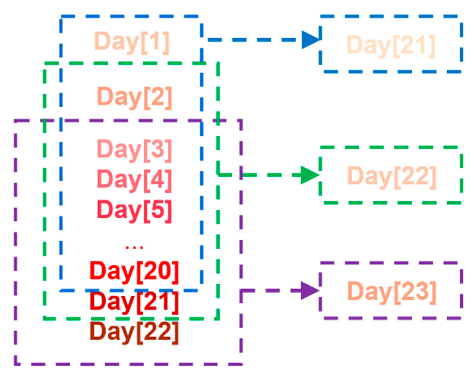
In this study, we used the forecasting method of a rolling time window that keeps the training interval unchanged and continuously rolls to forecast the volatility of the next day. As shown in Figure 5 (taking a window of 20 days as an example), if the time window is s days, the data from day t to day t + s are used to forecast the day t + s + 1, and the data from day t + 1 to day t + s + 1 are used to predict the day t + s + 2… to transform the input of two-dimensional index into three-dimensional data (the format is number of rows, time step, number of columns) for the rolling forecasting.

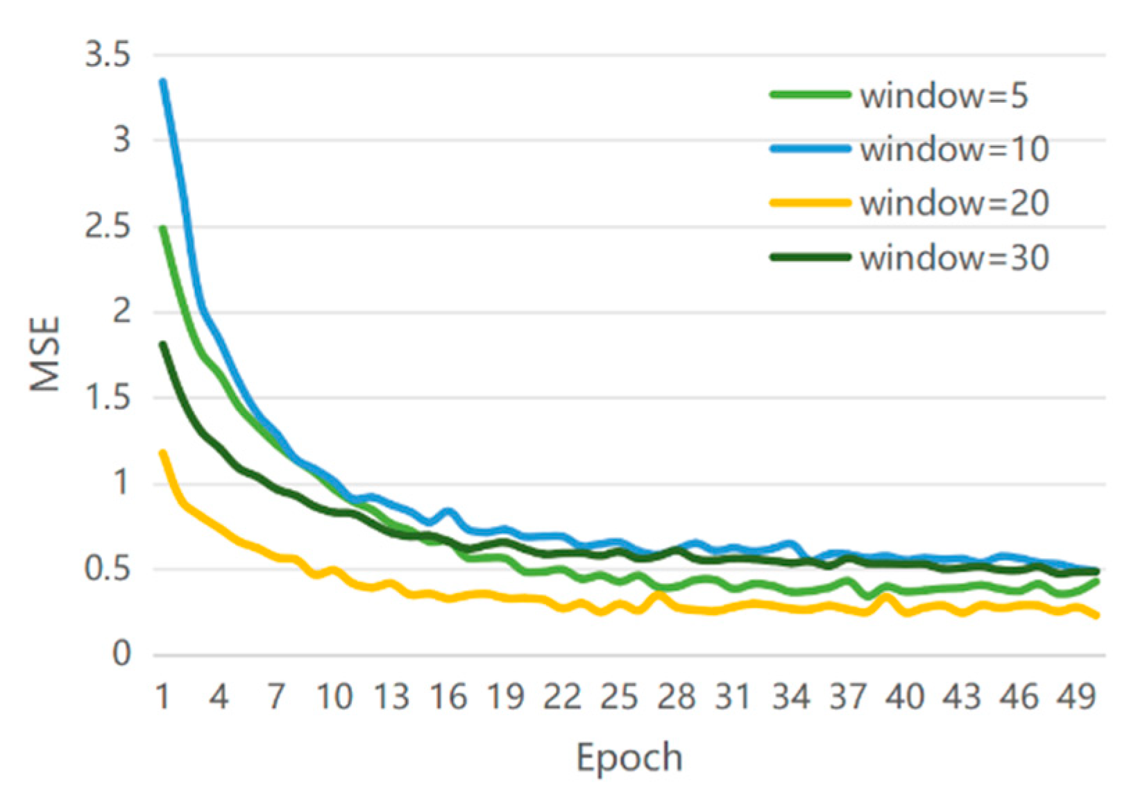
In order to analyze the influence of the width of time window on the prediction effect of the TCN model with the investor attention factor, we selected a time window of 5 days, 10 days, 20 days, and 30 days to construct the training data. The corresponding MSE is shown in Figure 6.

Through the error results of test set for different time windows, it can be found that the model has the strongest predictive ability when the time window value is 20. The reason for this result may be that if the time window is too large and contains relatively irrelevant data, the efficiency of training is greatly reduced, whereas if the time window is too small to ignore the data with a strong correlation with the explained variable, the results are unsatisfactory. The 20-day time window has the lowest test set error, which meets the needs of model training without causing too much redundant information. We use the data of the first 20 days to forecast the stock price volatility on the 21st day in order to achieve a balance between model calculation efficiency and effect.

The neural network framework in this study is implemented by the Keras framework in Python. In the image field, we often convolved two-dimensional data and the convolution of the time series is the convolution of one-dimensional data. In order to ensure the same size of the input and output of the convolution, the one-dimensional fully convolutional network (FCN) structure was used to cut off the redundant padding after the one-dimensional convolution; then, we performed two layers of one-dimensional convolution, and used ReLU to fit the nonlinear function relationship between the data. In order to ensure each convolution output contained more information and ensure that the long history information is not missed, a causal convolution with a dilation rate is used. The dilation rate of the first layer is 1 and the dilation rate of each layer is twice that of the previous layer. In order to solve the problem of gradient disappearance caused by the model being too deep, the residual block jump layer connection is used to replace the simple connection between each layer. The hyperparameter selection of TCN is shown in

Table 6. Model hyperparameter selection.

Parameters	Value	Parameters	Value
Training set	68%	Activation	ReLU
Filters	11	Loss function	mse
Convolution kernel	2	Batch size	84
Validation set	17%	Epoch	50
Testing set	15%	Metrics	‘mse,’‘mae,’‘rmse,’‘mape,’‘msle’
Optimizer	Adam	Windows Width	20 days

.

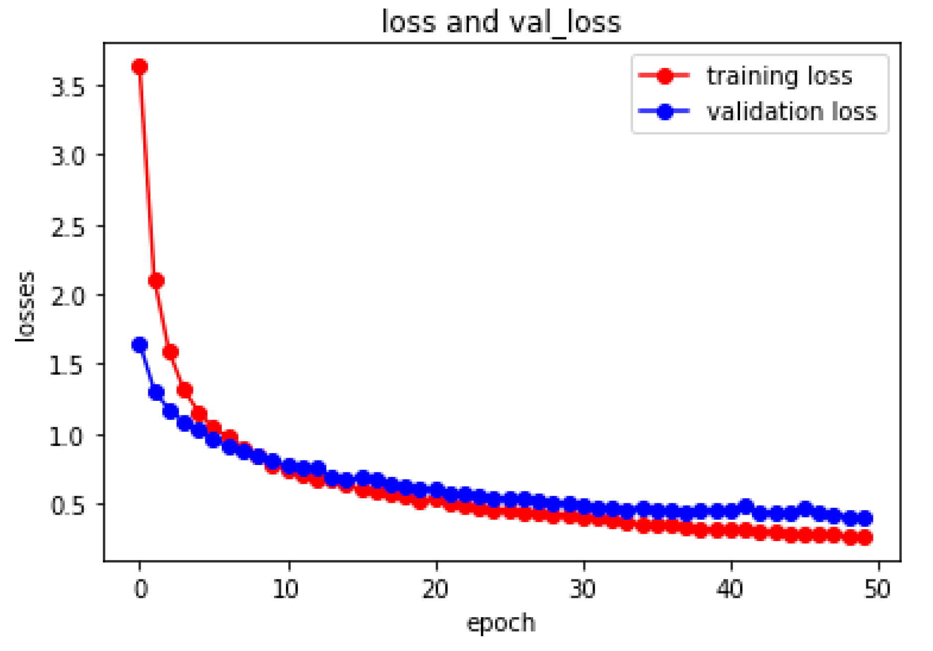
The change trend of the loss function for TCN model during the training process is shown in Figure 7.

3.4. Comparison of Model Prediction Accuracy

In this study, we compared the out-of-sample forecasting capabilities of nine volatility forecasting models under five evaluation criteria. Traditional econometric models include the GARCH and FIGARCH models under both normal distribution and t distribution, the ARFIMA model, and the HAR-RV model. Deep learning models include the LSTM model with investor attention factor and TCN models before and after adding investor attention factor. In order to explain the difference of different models, the p-statistics of the Kolmogorov–Smirnov (KS) test for different models were investigated, which are shown in

Table 7. Kolmogorov–Smirnov (KS) test results of different models.

	TCN + B	LSTM + B	GARCH-T	GARCH-N	FIGARCH-T	FIGARCH-N	ARFIMA	HAR-RV
TCN + B	1.00
LSTM + B	0.00	1.00
GARCH-T	0.00	0.00	1.00
GARCH-N	0.00	0.00	0.00	1.00
FIGARCH-T	0.00	0.00	0.00	0.00	1.00
FIGARCH-N	0.00	0.00	0.00	0.00	0.00	1.00
ARFIMA	0.00	0.00	0.00	0.00	0.00	0.00	1.00
HAR-RV	0.00	0.00	0.00	0.00	0.00	0.00	0.00	1.00

Note: Because TCN and TCN + B with investor attention factor are essentially the same model, only TCN + B model is listed in KS test table. GARCH-T and GARCH-N represent the generalized autoregressive conditional heteroscedasticity (GARCH) model under the t distribution and the normal distribution, respectively, and the FIGARCH models are the same. HAR-RV represents the heterogeneous autoregressive model of realized volatility. ARFIMA represents the model of autoregressive fractionally integrated moving average.

. From the statistical data, one can see that the p-values of the test for model differentiation between each model and itself are 1 and those between different models are approximately 0. The p-value of the test between different models is less than 0.05, which rejects the null hypothesis and means that the two groups of data do not follow the same distribution; that is, the difference between the two models is large.

Table 8. Prediction error of each model (step size is 1).

	TCN + B	TCN	LSTM + B	GARCH-T	GARCH-N	FIGARCH-T	FIGARCH-N	ARFIMA	HAR-RV
MSE	0.254	0.347	0.393	1.738	1.603	1.901	1.683	0.427	0.500
RMSE	0.504	0.589	0.627	1.318	1.266	1.379	1.297	0.653	0.707
MAE	0.331	0.364	0.378	1.077	1.030	1.086	1.045	0.326	0.399
MAPE	199.648	225.211	227.969	273.419	261.390	266.111	262.117	440.965	291.732
MSLE	0.045	0.052	0.053	0.314	0.296	0.315	0.301	0.081	0.070

Note: TCN + B represents the TCN model embedded with the investor attention factor. GARCH-T and GARCH-N represent the generalized autoregressive conditional heteroscedasticity (GARCH) model under the t distribution and the normal distribution, respectively, and the other GARCH family models are the same.

contains the out-of-sample prediction error of each model’s one-step forecasting and shows the accuracy ranking of every model under different evaluation criteria. The accuracy of the TCN after adding the investor attention factor is ranked first, and it is higher than that of the TCN without the investor attention factor, while its error is lower than that of the LSTM with the investor attention factor added. In addition, compared with the traditional econometric models, the deep learning models are significantly more accurate in volatility forecasting. After adding the investor attention factor, under the five evaluation criteria including MSE, RMSE, MAE, MAPE, and MSLE, TCN increased by 13%, 7%, 5%, 7%, and 12%, respectively; the TCN without the investor attention factor increased by 11%, 6%, 4%, 1%, 14%, and 3% compared with the LSTM with the investor attention factor added.

Traditional econometric models only consider the historical information of volatility and use linear functional relationships, while the deep learning models consider the historical information of volatility and use other indicators that affect volatility changes. In addition, the deep learning models consider more about the influence of trading information and external factors and the nonlinear relationships between variables, so they have higher accuracy in volatility forecasting.

The investor attention factor synthesized by the Baidu search index reflects the public’s attention in various fields, including traders’ interest in the stock industry, types of stocks, etc. It has good significance for predicting the macro situation and the overall sentiment orientation of investors. After joining the Baidu search index, the TCN model considers the transaction information and forecasts the macro situation according to the hot spots of investors’ attention, making the volatility forecasting index system more complete; therefore, after adding the Baidu search index, the improved prediction accuracy was in line with our expectations.

Compared with LSTM, the deep learning model TCN can process sequence information in parallel instead of sequential processing, which can flexibly adjust the size of the receptive field, requires smaller memory, and has a more stable gradient than recurrent neural networks; therefore, in the case of the embedding investor attention factor, TCN has a stronger out-of-sample predictive ability than LSTM.

Based on the one-step forecasting results, we conduct the two-step prediction and five-step prediction to test the robustness of the experimental results.

Table 9. Prediction error of each model (step size is 2).

	TCN + B	TCN	LSTM + B	GARCH-T	GARCH-N	FIGARCH-T	FIGARCH-N	ARFIMA	HAR-RV
MSE	0.270	0.372	0.435	1.876	1.724	1.913	1.784	0.637	0.602
RMSE	0.519	0.610	0.660	1.370	1.313	1.383	1.336	0.798	0.776
MAE	0.325	0.411	0.366	1.118	1.066	1.092	1.083	0.468	0.492
MAPE	184.693	224.922	197.097	282.495	268.879	267.997	272.226	74.360	120.588
MSLE	0.070	0.077	0.098	0.331	0.311	0.318	0.318	0.147	0.099

and

Table 10. Prediction error of each model (step size is 5).

	TCN + B	TCN	LSTM + B	GARCH-T	GARCH-N	FIGARCH-T	FIGARCH-N	ARFIMA	HAR-RV
MSE	0.526	0.572	0.593	2.070	1.884	2.111	1.958	0.685	0.633
RMSE	0.725	0.756	0.776	1.439	1.373	1.453	1.399	0.827	0.796
MAE	0.465	0.478	0.500	1.183	1.123	1.153	1.143	0.574	0.458
MAPE	221.514	241.448	248.170	305.385	288.811	288.172	293.086	151.824	72.207
MSLE	0.090	0.099	0.101	0.366	0.341	0.349	0.349	0.129	0.144

show the error and the accuracy ranking of each traditional econometric model and deep learning model in two-step prediction and five-step prediction, respectively.

Observing the prediction errors and accuracy rankings of models in different step sizes, we found that the accuracy ranking of each model is relatively stable. The rankings of deep learning models are always higher than the traditional econometric models. Among them, the TCN is more robust than the LSTM, and the accuracy of the LSTM in the five-step prediction ranks slightly behind the HAR-RV model, whereas the TCN maintains the highest accuracy under three kinds of step sizes. Through further comparison, it can be found that the TCN, after adding the investor attention factor, maintains the lowest error in the volatility forecasting under three different step sizes, indicating that the investor attention factor has a certain positive effect on the volatility forecasting.

4. Discussion

By calculating the time difference correlation coefficient, we can get the antecedent, consistency, or lag of a certain economic index series to the benchmark index; however, other correlation coefficients cannot obtain the time difference of the two indexes. In predicting economic indicators, it is more significant to use the indicators that are ahead of the benchmark indicators.

In order to show that the conclusions of this study are valid under different calculation methods of the correlation coefficient, we will discuss the cross-correlation coefficient to filter keywords, and then recalculate the weight of each keyword after filtering and synthesize daily investor attention factor based on the cross-correlation number according to the method of Section 3.2.3. The steps are as described in the next sections.

4.1. Construct the Attention Factor by Using the Cross-Correlation Coefficient

We calculated the cross-correlation coefficient between each keyword and volatility in the initial keyword database, comprehensively considered its significance and the value of the cross-correlation coefficient, and selected 12 keywords that were highly correlated with volatility. The value of the cross-correlation coefficient is shown in

Table 11. Keywords selected by the cross-correlation coefficient.

Keywords	Coefficient	Keywords	Coefficient
Shopping	0.298 **	Education	0.177 **
Financial Crisis	0.280 **	Bankruptcy	0.168 **
E-Commerce	0.241 **	Small and Medium-sized Enterprises	0.123 **
Financial Investment	0.237 **	Real Estate	0.122 **
Aviation	0.202 **	Travel	0.122 **
Credit Card	0.190 **	Cell Phone	0.104 **

Note: “Coefficient” represents cross-correlation coefficient. ** indicates significant correlation at 0.01 level.

.

Then, the cross-correlation coefficient of the above keywords was normalized, and the processed value was taken as the corresponding weight of the keywords. The index of 12 keywords in a day is multiplied by the corresponding weight, and the investor attention factor based on the cross-correlation coefficient of the day is obtained. The investor attention factor based on the time-difference correlation coefficient of the TCN model in this study is replaced by the attention factor based on the cross-correlation coefficient for further prediction. The error between the TCN model and other models is shown in

Table 12. Comparison between attention factor model based on cross-correlation coefficient and other models.

	TCN + B	TCN	LSTM + B	GARCH-T	GARCH-N	FIGARCH-T	FIGARCH-N	ARFIMA	HAR-RV	TCN + C
MSE	0.302	0.347	0.393	1.738	1.603	1.901	1.683	0.427	0.500	0.308
RMSE	0.549	0.589	0.627	1.318	1.266	1.379	1.297	0.653	0.707	0.555
MAE	0.347	0.364	0.378	1.077	1.030	1.086	1.045	0.326	0.399	0.335
MAPE	209.204	225.211	227.969	273.419	261.390	266.111	262.117	440.965	291.732	218.455
MSLE	0.045	0.052	0.053	0.314	0.296	0.315	0.301	0.081	0.070	0.049

Note: TCN + C represents the TCN model embedded with investor attention factor constructed through the cross-correlation coefficient of keywords.

.

Table 12 shows that adding the Baidu Index filtered by other correlation coefficients to the TCN model can also improve the ability of forecasting volatility; however, the effect of the cross-correlation functions on the TCN model is worse than the effects by the time-difference correlation on the TCN model. The cross-correlation function describes the correlation between time series at any two different moments t₁ and t₂. It may result in future data being used to predict previous data, which is not reasonable.

4.2. Construct the Attention Factor by Using the Correlation Coefficient with RV

We did not consider the delay order of the time difference correlation coefficient, and used the RV correlation coefficient to filter keywords; that is, the filtering of keywords is only related to the absolute value of the correlation coefficient. We selected 12 keywords with a high correlation coefficient absolute value. The selected keywords are shown in

Table 13. Keywords selection based on the realized volatility (RV) correlation coefficient.

Keywords	Order	Coefficient	Keywords	Order	Coefficient
Shopping	5	0.333 **	Bankruptcy	−20	0.173 **
Financial Crisis	1	0.333 **	Travel	7	0.135 **
E-Commerce	3	0.274 **	Small and Medium-sized Enterprises	−6	0.132 **
Financial Investment	−1	0.235 **	Real Estate	4	0.127 **
Aviation	−4	0.228 **	Cell Phone	2	0.107 **
Credit Card	−7	0.196 **	Car	1	0.102 **

Note: “Order” represents the time delay order. “Coefficient” represents the maximum correlation coefficient. ** indicates a significant correlation at 0.01 level.

. According to the method of Section 3.2.3, these keywords are combined into investor concern factors to replace the original concern factors based on the time difference correlation coefficient, and put into different models for further prediction. The errors of different models are shown in

Table 14. The error comparison between the TCN model with attention factor based on the RV correlation coefficient and other models.

	TCN + B	TCN	LSTM + B	GARCH-T	GARCH-N	FIGARCH-T	FIGARCH-N	ARFIMA	HAR-RV	TCN + N
RMSE	0.549	0.589	0.627	1.318	1.266	1.379	1.297	0.653	0.707	0.605
MAE	0.347	0.364	0.378	1.077	1.030	1.086	1.045	0.326	0.399	0.368
MAPE	209.204	225.211	227.969	273.419	261.390	266.111	262.117	440.965	291.732	211.923
MSLE	0.045	0.052	0.053	0.314	0.296	0.315	0.301	0.081	0.070	0.048

Note: The TCN + N model in the table represents the TCN model with investors’ attention factor added based on keyword filtering method without considering delay order.

.

Table 14 shows that the prediction effect of the TCN model based on the realized volatility (RV) correlation coefficient is not good because it does not consider the delay order between indicators. The TCN model based on the time-difference correlation coefficient considering delay order has higher prediction accuracy; however, no matter what kind of keyword filtering method is added to the TCN model, the accuracy of volatility prediction is higher than that of ordinary the TCN model and the LSTM + B model.

4.3. Limitations and Shortcomings

Our study has two major scientific weakness: (1) We cannot compare our results with other search data across countries (Google etc.). Consequently, the results are neither generalizable nor robust given the limitation of utilizing only Baidu search data. (2) Our search data (Baidu) and the search engine process might be manipulated for certain reasons. Thus, the data could be biased without our knowledge and this might affect the results.

5. Conclusions and Extension

In this study, we constructed an investor attention factor through the Baidu search antecedent keyword index, and analyzed other trading information of the Volatility Prediction by combining high-frequency financial data and the deep learning TCN model. Compared with traditional econometric models, such as GARCH and FIGARCH models with normal and t-distribution error terms, ARFIMA and HAR-RV models, and the deep learning LSTM model, we found that the investor attention factor based on the TCN model has a higher prediction accuracy for out-of-sample volatility and has better sustainability and robustness under five loss functions. The results show that investors’ attention factor has a positive impact on the accuracy of Volatility Prediction. This study provides a more accurate and robust method for Volatility Prediction and expands the application scope of deep learning. The improved model can also be used to predict individual stocks, which can provide reliable guidance for preventing risks and obtaining returns.

In future work, we can improve three aspects. First, we can enrich the index system of volatility prediction and introduce external news text; second, we will try to provide a mathematical or statistical basis for the method proposed in this paper; third, we will use the Black Scholes model to calculate the implied volatility (IV) and use IV (lagged) as a substitute predictor or combined with investors’ attention factor in order to improve the prediction accuracy.