1. Introduction
Lattice-based cryptography is one of the most widely and deeply studied post-quantum cryptography. Discrete Gaussian sampling is one of the important mathematical tools for lattice-based cryptography [
1,
2,
3]. Many lattice-based cryptosystems, including their security proofs, involve discrete Gaussian sampling.
Generally, discrete Gaussian sampling is to sample from a (multivariate) discrete Gaussian distribution over an
n-dimensional lattice
. In particular, discrete Gaussian sampling over the integers, denoted by
, refers to the generation of random integers that conform to Gaussian distribution
with parameter
and center
. Since
is much more efficient and simpler than discrete Gaussian sampling over a general lattice, many lattice-based cryptosystems, such as [
4,
5], only involve discrete Gaussian sampling over the integers.
The methods of sampling from a continuous Gaussian distribution are not trivially applicable for the discrete case. Therefore, it is of great significance to study discrete Gaussian sampling and design sampling algorithms, especially for . This issue has attracted a lot of attention in recent years.
1.1. Related Work
For the commonly used methods (techniques) for
, including inversion sampling, the Knuth-Yao method and the rejection sampling, we can refer to [
6,
7]. One can also consider the convolution technique (based on the convolution-like properties of discrete Gaussian developed by Peikert in [
8]) [
9,
10]. In addition, Saarinen developed a new binary arithmetic coding sampler for discrete Gaussians (BAC Sampling) [
11]. Moreover, Karmakar et al. designed a class of very efficient discrete Gaussian samplers based on computing a series of Boolean functions with a number of random bits as the input [
12,
13].
Sampling from a discrete Gaussian distribution over the integers usually involves floating-point arithmetic because of the exponential computation in Gaussian function. It is believed that high-precision floating-point arithmetic is required for attaining enough statistical distance to the target distribution. This implies that online high-precision floating-point computation may be an implementation bottleneck. Thus, we can see that most of the improved
algorithms manage to use high-precision floating-point arithmetic only at offline time (such as algorithms based on CDT’s or Knuth-Yao) or even to avoid floating-point arithmetic (such as Karney’s sampling algorithm [
14]).
Recently results show that the Bernoulli sampling, introduced by Ducas et al. in [
4] for centered discrete Gaussian distributions over the integers, can be effectively improved by combining the polynomial approximation technique. Specifically, Bernoulli sampling is a kind of rejection sampling. Its rejection operation can be done very efficiently by calculating an approximated polynomial [
15,
16]. The polynomial is predetermined; it thus supports discrete Gaussians with a varying center
over the integers.
Generic discrete Gaussian sampling algorithms over the integers that support a varying center
and even a varying parameter
are also very interesting. A discrete Gaussian sampling algorithm for an
n-dimensional lattice usually requires such an algorithm as its subroutine [
2,
8,
17,
18]. However, most of the algorithms for sampling
and their improvements are designed only for the case where center
is fixed in advance, such as [
4,
9,
11,
19,
20]. When sampling from
with varying
(e.g., double-precision numbers that are sampled from a specific distribution online), except [
14], the existing algorithms available rely on floating-point arithmetic, such as the algorithms in [
2,
15] and the sampler used in Falcon signature [
5] or require a large amount of offline computation and precomputation storage, such as the algorithms proposed by Micciancio et al. [
10] and by Aguilar-Melchor et al. [
21] respectively. Moreover, the sampler presented by Barthe et al. in [
16] is not a generic algorithm, as it supports a varying
but not a varying parameters
. One needs to determine a new approximation polynomial for each new
.
1.2. Our Contribution
In this paper, combining the idea of Karney’s algorithm for sampling the Bernoulli distribution , we present a generalized version of Bernoulli sampling algorithm for both centered and noncentered discrete Gaussian distributions over the integers (see Algorithm 1).
Specifically, we present an improved implementation of the Bernoulli sampling algorithm for centered discrete Gaussian distributions over the integers (see Algorithm 2). We remove the precomputed table, that is required and obtained by using floating-point arithmetic in advance in the original Bernoulli sampling algorithm. Except a fixed look-up table of very small size (e.g., 128 bits) that stores the binary expansion of , our proposed algorithm requires no precomputation storage and uses no floating-point arithmetic.
We also propose a noncentered Bernoulli sampling algorithm (see Algorithm 3) that supports discrete Gaussian distributions with varying centers. It uses no floating-point arithmetic, and it is suitable for sampling
with
of precision up to 52 bits. We also show that our noncentered version of sampling algorithm has the same rejection rate as the original Bernoulli sampling algorithm. Furthermore, the experimental results show that our proposed algorithms have a significant improvement in the sampling efficiency as compared to other rejection algorithms for discrete Gaussian distributions over the integers [
14].
Table 1 summarizes the some existing sampling algorithms for discrete Gaussian distributions over the integers and their properties in comparison to our work. Here,
is the security parameters. The column “FPA” and the column “
” indicate if the algorithm requires to use floating-point arithmetic online and to evaluate
online respectively. The column “varying
” refers to the property of being able to produce samples (online) from discrete Gaussians with varying centers rather than a specific discrete Gaussian with a fixed center. Similarly, the column “varying
” refers to the property of being able to produce samples (online) from discrete Gaussians with varying parameter
.
2. Materials and Methods
2.1. Preliminaries
In this paper, denotes the set of real numbers, and denotes the set of integers and non-negative integers respectively. We use to define any real function to a countable set S if it exists, and use to define the Gaussian function evaluated at , where parameter and center . Besides, defines the discrete Gaussian distribution evaluated at , where , , .
Bernoulli(-type) sampling algorithm proposed by Ducas et al. in [
4] was designed exclusive for a centered discrete Gaussian distribution over the integers, namely
with
and
, where
k is a positive integer and
. This algorithm uses rejection sampling from the
binary discrete Gaussian distribution, denoted by
. Sampling from
can be very efficient using only unbiased random bits (one may refer to Algorithm 10 in [
4]). Firstly, it samples an integer
from
, then samples
uniformly in
and accepts
with probability
, finally, it outputs a signed integer,
z or
, with equal probabilities because of the symmetry of the target distribution (see Algorithm 11 and Algorithm 12 in [
4]). It was shown that the average number of rejections is not more than
.
A precomputed look-up table is required for computing the exponential function
. The size of the table varies with the parameter
. For examples, the size is
kb for
and 4 kb for
according to the estimations given by Ducas et al. in [
4], which is not very small but acceptable.
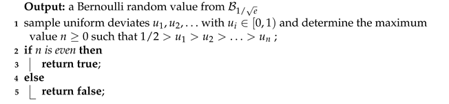
Algorithm 1 is adapted by Karney [
14] from Von Neumann’s algorithm that samples from
, where
. Algorithm 1 is used as one of the basic operations in Karney’s sampling algorithm for the standard normal distribution, which can be executed only by using integer arithmetic.
In Algorithm 1, by replacing
with
, we can get a Bernoulli random value. The value is true with probability
, namely sampling from
, where
are positive integers and
. The above modification can be regarded as a generalized version of Algorithm 1, which is used implicitly in Karney’s algorithm. The discrete Gaussian distribution over integers in Karney’s algorithm also adopts the rejection sampling algorithm, which is a discretization of Karney’s algorithm for sampling from the standard normal distribution. It is fit for discrete Gaussians with varying rational parameters of precision up to 32 bits (including
and
). The algorithm does not require any floating-point arithmetic. Moreover, it needs no precomputation storage. One may refer to [
14] for the full description of Karney’s sampling algorithm.
| Algorithm 1: [14] Sample from Bernoulli distribution |
![Mathematics 09 00378 i001]() |
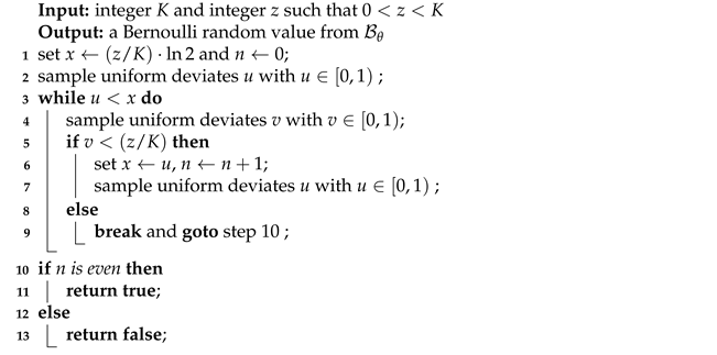
2.2. Removing Precomputed Tables in Bernoulli Sampling
One drawback of the Bernoulli sampling is that it needs a precomputed table to generate a Bernoulli random value from . Although the table is not large, it has to be precomputed before sampling for every different . Therefore, it is interesting to sample without a precomputed table. In this subsection, we propose an alternative algorithm, which samples for a given and does not require a precomputed table except a fixed look-up table with small size.
We use the notation of the sampling algorithm given by Ducas et al. (Algorithm 11 in [
4]). Since
and
, it follows that
is equal to
where
is the fractional part of
. Then the Bernoulli value can be obtained by generating
Bernoulli deviates according to
and one Bernoulli random value from
. If no false value is generated in this procedure, then we have
true, otherwise we have
false.
It is clear that a Bernoulli deviate according to is equivalent to a uniform random bit. Thus, the only remaining problem is to generate a Bernoulli random value from . We address this problem via Algorithm 2.
One can see that Algorithm 2 is adapted from Algorithm 1. It provides a technique for determining the relation between and a uniform deviate , and it does not need floating-point operations during run-time, if the binary expansion of , that is long enough (e.g., 128 bits), has been stored as a fixed look-up table.
In step 1,
p is assigned to be the
t most significant bits of the binary expansion of
. In steps 5 and 6, if
, then we have
, which follows that
. It is equivalent to obtaining a uniform deviate
that is strictly less than the value of
. On the contrary, in steps 7 and 8, if
, then it is equivalent to obtaining a uniform deviate
that is strictly more than the value of
. Otherwise, if
, i.e.,
. This means that we get a uniform deviate
, but in this moment we cannot determine whether it is less than the value of
or not.
| Algorithm 2: Sample from Bernoulli distribution , where are positive integers such that |
![Mathematics 09 00378 i002]() |
In Algorithm 2, the while loop is designed to further compare the uniform deviate with the value of
. Informally, if
for some
, then we generate another uniformly random integer
, which means that we get a uniform deviate
. When comparing
with
, if
then we have
, which follows that
. Since
, we have
if
i.e.,
which is equivalent to
where
is the fractional part of the rational number
, which can be determined by computing
. Therefore, as presented in Algorithm 2, after steps 9, 10, and 11 what we get is actually
and
. So, we can continue to compare the uniform deviate
with the value of
. For the full proof of the correctness, one may refer to
Appendix A.
2.3. Bernoulli Sampling for Discrete Gaussians with Varying Centers
In this subsection, we propose a new noncentered Bernoulli sampling algorithm for
with
, where
b is a power of two,
,
k is a positive integer,
. Our proposed algorithm does not require any floating-point arithmetic, and it needs no precomputed table except a fixed and small size look-up table for storing the binary expansion of
, as mentioned in
Section 2.2.
Informally, the sketch of the proposed algorithm is as follows. We sample an integer
from
firstly, and then sample
uniformly in
. Since the symmetry of a noncentered discrete Gaussian distribution does not hold, we need to determine the sign of prospective output before the acceptance-rejection operation, by setting
with equal probabilities. Finally, we accept
as the output with probability
and restart the whole algorithm if otherwise, where
. The following equation
guarantees that the output value has the desired relative probability density
. The sketch of the algorithm seems to work, but there are several subtleties we have to address.
Bernoulli sampling for centered discrete Gaussian distributions needs to restart its whole sampling procedure with probability
when the algorithm is about to return
(see Algorithm 12 in [
4]). In our algorithm, in order to avoid double counting 0, we need to set
if
, so that there is only one case where
. This also guarantees that
is always non-negative, and thus
is never more than one.
Another problem is how to compute the value of the exponential function efficiently. Since
and
with
, it follows that
where
and
is the fractional part of
. Then, when computing the value of exponential function
, we generate
Bernoulli deviates according to
and one Bernoulli random value which is true with probability
. If no false value is generated, then we accept
as the output, otherwise we restart the algorithm. In summary, our proposed algorithm can be formally described as Algorithm 3, which summarizes the above discussion.
Recall that our goal is to give an algorithm that requires no floating-point arithmetic. It is clear that a Bernoulli deviate according to
is equivalent to a uniform random bit, and sampling from
can be efficiently implemented by using only unbiased random bits (Algorithm 10 in [
4]). Thus, the only remaining problem is to generate a Bernoulli random value with probability
without using floating-point arithmetic. Since
is a non-negative integer, what we need essentially is a solution for generating a Bernoulli random value from
, where
and
k are positive integers such that
. To end this, we can apply Algorithm 2 by replacing
k with
, which involves no floating-point arithmetic and requires no precomputation storage.
| Algorithm 3: Sample from discrete Gaussian distribution for , and |
![Mathematics 09 00378 i003]() |
Moreover, let and , then we have and with overwhelming probability. This means that Algorithm 3 supports a of precision up to 20 bits if k is restricted to be less than , and it can be implemented only by using 64-bit integer arithmetic.
A sampler for centers of low precision can be used in q-ary lattices, where q is relatively large but not very large, and sampling from discrete Gaussian distributions with q different centers may be required in this case. It involves a large storage requirement if one uses precomputed tables. So, one could consider our sampler as described in Algorithm 3. It requires no precomputed table.
2.4. Increasing the Precision of
Algorithm 3 only supports centers of finite precision. The precision of depends on the value of b. A larger b means a of higher precision. For example, let . We remark that the bound of 52 bits is significant. We note that float-pointing with 53 bits of precision corresponds to the double precision type in the IEEE 754 standard, and it is usable in software. When is given by a double-precision floating-point number, we could represent as a rational number of denominator and use Algorithm 3 directly.
However,
b cannot be
in practice, since in this case we need to compute
where
, which leads to the integer overflow (for 64-bit C/C++ compilers). A big integer library works but compromises the performance at runtime. In this subsection, therefore, we try to improve Algorithm 3 so that it supports a
of precision up to 52 bits.
The basic idea is to avoid compute
. We note that generating a Bernoulli random value which is true with probability
can be decomposed to generating two Bernoulli random values which are true with probability
and
respectively. It is not hard to see that a Bernoulli random value which is true with probability
can be generated by using Algorithm 2 with
and
. In particular, Algorithm 2 requires
. When
, we need to compute
and invoke Algorithm 1 firstly, and then use Algorithm 2 with
and
.
The following algorithm is designed to generate a Bernoulli random value from Bernoulli distribution
with
. As the inequality
holds except
and
,
can be calculated by using Algorithm 4 with
and
.
| Algorithm 4: Sample from Bernoulli distribution with and |
![Mathematics 09 00378 i004]() |
The main idea behind Algorithm 4 is to sample two sets of uniform deviates
and
, and to decide the maximum value
such that
and
. Then, the probability that
n is even, which means it returns
true, is given by
Furthermore, when implementing Algorithm 4, we need to apply the technique presented in Algorithm 2 for comparing u with and avoiding using floating-point arithmetic.
Let us go back to the problem of increasing the precision of . If k is restricted to be less than , we can take . In this case, we have and with overwhelming probability. This means that Algorithm 3, incorporated with Algorithm 4 as well as Algorithm 2, supports a of precision up to 52 bits if k is restricted to be less than , and it can be implemented only by using 64-bit integer arithmetic.
3. Results
On a laptop computer (Intel i7-8550U, 16 GB RAM, the g++ compiler and enabling -O3 optimization option), we implemented GPV algorithm in [
2], Karney’s algorithm in [
14], the original Bernoulli sampling algorithm in [
4], and our Algorithm 3 respectively. Except Karney’s algorithm, the uniformly pseudorandom numbers are generated by using AES256-CTR with AES-NI (Intel Advanced Encryption Standard New Instructions).
Figure 1 shows the performance comparison of these sampling algorithms.
We select Karney’s algorithm and the GPV algorithm to compare with our generalized Bernoulli sampling because they also use rejection sampling and requires no precomputation storage. Although algorithms based on the inversion sampling or Knuth-Yao method are usually more efficient, they require a large amount precomputation storage, especially for sampling from distributions with variable or large .
For centered discrete Gaussian distributions with roughly from 10 to 190, one can get about samples per second by using Algorithm 3. This means that the performance of our improved Bernoulli sampling algorithm is significantly better than the original Bernoulli sampling as well as Karney’s sampling algorithm. When , for the discrete Gaussian distribution with and i uniformly from , we also tested that Algorithm 3 has almost the same performance as the case of centered discrete Gaussian distributions. When we take , we need combine Algorithm 4 to implement Algorithm 3. The performance in this case decreases to about per second and is slightly worse than the original Bernoulli sampling algorithm, but the latter does not support noncentered discrete Gaussian distributions.
Here, the GPV algorithm has the worst performance, since its proposal distribution is poor and its rejection rate is too high, which is close to 10 [
2], while the Bernoulli sampling algorithm has a rejection rate of about
, and the rejection rate of Karney’s algorithm is even as lower as
[
14]. We will prove in
Section 4 of this paper that the rejection rate of Algorithm 3 is still about
.
Our Algorithm 3 has a better performance than Karney’s algorithm, this is due to the fact that it uses the binary discrete Gaussian distribution as its base sampler instead of , and there exists a very efficient sampling algorithm for such a discrete Gaussian distribution. Algorithm 3 is faster than the original Bernoulli sampling algorithm, mainly because its rejection operation is simplified to sample from only one Bernoulli distribution with an exponential function as its parameter, while the original Bernoulli sampling algorithm requires a lookup table to sample a relatively large number of Bernoulli distributions with exponential functions as parameters in order to perform the rejection operation, which affects its practical performance.
Note that our Algorithm 4 requires Algorithm 2 to be fully implemented, and the basic idea of Algorithm 4 follows from that of Algorithm 2. We perform algorithm 4 once roughly as the same amount of computation as Algorithm 2 twice. This helps us intuitively explain why the performance of Algorithm 3 drops by about half after using Algorithm 4.
4. Discussion
In this section, we show that the noncentered version of Bernoulli sampling presented by Algorithm 3 has the same rejection rate as the Bernoulli sampling for centered discrete Gaussians.
Intuitively, evaluating the rejection rate of Algorithm 3 could be done just as evaluating the rejection rate of Bernoulli sampling for centered discrete Gaussian distributions, which has been presented by Ducas et al. in [
4]. Notwithstanding, we may need the notion of the smoothing parameter of lattices, which was introduced by Micciancio and Regev in [
1], because of the noncentered discrete Gaussian distributions. In fact, we only need the notion of smoothing parameter of lattice
and its two important properties, since this work only involves the (one-dimensional) integer lattice
, which is the simplest lattice.
Definition 1 (a special case of [
1], Definition 3.1)
. Let be a positive real. The smoothing parameter of lattice , denoted by , is defined to be the smallest real s such that . Lemma 1 (a special case of [
1], Lemma 3.3)
. For any real , the smoothing parameter of lattice satisfies . Lemma 2 (Ref. [
1], Lemma 2.8, implicit)
. For any (small) real and , if , then , and . Theorem 1. For Algorithm 3, if , then the expected number of rejections that it requires is not more than .
Proof. From the perspective of rejection sampling, for Algorithm 3, the proposal distribution density function is
and the target distribution density function
f can be written as
where
,
and
. The expected number of rejections that the algorithm requires can be evaluated by
If
, then
(or
when
). Then we have
where the two approximate equality symbols follow from Lemma 2. This completes the proof. □
We remark that Theorem 1 holds for in practice. In the proof of Theorem 1, taking we have , which guarantees that gets close enough to by Lemma 2. According to Lemma 1, we get with .
We can also see that the rejection rate of also represents the average number of times that Algorithm 3 calls Algorithm 2 or Algorithm 4. This is because the rejection rate of Algorithm 3 is actually equal to the inverse of the probability that the algorithm executes step 7 and step 10 without restarting. Algorithm 3 needs to perform step 7 whenever it successfully outputs the sample or restarts, and step 7 requires a call to Algorithm 2 or Algorithm 4. Thus, the average number of times that step 7 is executed is the rejection rate, and the average number of calls of Algorithm 2 or Algorithm 4 is thus the rejection rate, which is about and independent from the parameter and the center , according to Theorem 1.
5. Conclusions
In this paper, we show that the Bernoulli(-type) sampling for centered discrete Gaussian distributions over the integers can be implemented without floating-point arithmetic. Except a fixed look-up table of very small size (e.g., 128 bits) that stores the binary expansion of , our proposed algorithm does not need any precomputation storage and requires no floating-point arithmetic. We also present a noncentered Bernoulli sampling algorithm that satisfies the need of discrete Gaussian distributions with varying centers. The algorithm needs no floating-point arithmetic, and it is suitable for sampling with of precision up to 52 bits. The noncentered version of algorithm has the same rejection rate as the original Bernoulli sampling algorithm. The experiment shows that our improved algorithms have better performance as compared to other rejection algorithms for discrete Gaussian distributions over the integers.
Author Contributions
Conceptualization, Y.D.; methodology, Y.D.; software, Y.D.; validation, S.X. and S.Z.; formal analysis, Y.D. and S.Z.; investigation, S.X. and S.Z.; resources, S.X.; data curation, S.X.; writing—original draft preparation, Y.D.; writing—review and editing, S.X.; visualization, S.X. and S.Z.; supervision, Y.D.; project administration, Y.D.; funding acquisition, Y.D. All authors have read and agreed to the published version of the manuscript.
Funding
This research was funded by National Natural Science Foundations of China (Grant Nos. 61972431), Guangdong Major Project of Basic and Applied Research (2019B030302008), Guangdong Basic and Applied Basic Research Foundation (No. 2020A1515010687) and the Fundamental Research Funds for the Central Universities (Grant No. 19lgpy217).
Institutional Review Board Statement
Not applicable.
Informed Consent Statement
Not applicable.
Conflicts of Interest
The authors declare no conflict of interest. The funders had no role in the design of the study; in the collection, analyses, or interpretation of data; in the writing of the manuscript, or in the decision to publish the results.
Appendix A
Let
be
n integers such that
for each
. For
,
and
are defined as follows:
and
In particular,
and
.
Theorem A1. Let . Suppose thatfor each integer . If , then . If , then . Proof. Since
, we have
It follows that
and
Then, we have
as
. Thus, we have
If
, with similar arguments, applying
with
, we get
We continue working backwards until finally we obtain
which means that
It follows that
This is equivalent to obtaining a uniform deviate
which is strictly less than the value of
.
Similarly, if
for each integer
, but
Then, we essentially get a uniform deviate
that is strictly more than the value of
. □
References
- Micciancio, D.; Regev, O. Worst-Case to Average-Case Reductions Based on Gaussian Measures. SIAM J. Comput. 2007, 37, 267–302. [Google Scholar] [CrossRef] [Green Version]
- Gentry, C.; Peikert, C.; Vaikuntanathan, V. Trapdoors for hard lattices and new cryptographic constructions. In Proceedings of the STOC 2008, Victoria, BC, Canada, 17–20 May 2008; Dwork, C., Ed.; ACM: New York, NY, USA, 2008; pp. 197–206. [Google Scholar]
- Lyubashevsky, V.; Peikert, C.; Regev, O. On Ideal Lattices and Learning with Errors over Rings. J. ACM 2013, 60, 43:1–43:35. [Google Scholar] [CrossRef]
- Ducas, L.; Durmus, A.; Lepoint, T.; Lyubashevsky, V. Lattice Signatures and Bimodal Gaussians. In Proceedings of the CRYPTO 2013, Santa Barbara, CA, USA, 18–22 August 2013; Canetti, R., Garay, J.A., Eds.; Proceedings, Part I. Springer: Berlin/Heidelberg, Germany, 2013; Volume 8042, pp. 40–56. [Google Scholar]
- Prest, T.; Fouque, P.A.; Hoffstein, J.; Kirchner, P.; Lyubashevsky, V.; Pornin, T.; Ricosset, T.; Seiler, G.; Whyte, W.; Zhang, Z. Falcon: Fast-FourierLattice-Based Compact Signatures over NTRU. Technical Report. Specifications v1.1. Available online: https://falcon-sign.info/ (accessed on 8 January 2021).
- Folláth, J. Gaussian Sampling in Lattice Based Cryptography. Tatra Mt. Math. Publ. 2014, 60, 1–23. [Google Scholar] [CrossRef] [Green Version]
- Dwarakanath, N.C.; Galbraith, S.D. Sampling from discrete Gaussians for lattice-based cryptography on a constrained device. Appl. Algebra Eng. Commun. Comput. 2014, 25, 159. [Google Scholar] [CrossRef]
- Peikert, C. An Efficient and Parallel Gaussian Sampler for Lattices. In Proceedings of the CRYPTO 2010, Santa Barbara, CA, USA, 15–19 August 2010; Rabin, T., Ed.; Springer: Berlin/Heidelberg, Germany, 2010; Volume 6223, pp. 80–97. [Google Scholar]
- Pöppelmann, T.; Ducas, L.; Güneysu, T. Enhanced Lattice-Based Signatures on Reconfigurable Hardware. In Proceedings of the CHES 2014, Busan, Korea, 23–26 September 2014; Batina, L., Robshaw, M., Eds.; Springer: Berlin/Heidelberg, Germany, 2014; Volume 8731, pp. 353–370. [Google Scholar]
- Micciancio, D.; Walter, M. Gaussian Sampling over the Integers: Efficient, Generic, Constant-Time. In Proceedings of the CRYPTO 2017, Santa Barbara, CA, USA, 20–24 August 2017; Katz, J., Shacham, H., Eds.; Proceedings, Part II. Springer: Berlin/Heidelberg, Germany, 2017; Volume 10402, pp. 455–485. [Google Scholar]
- Saarinen, M.J.O. Arithmetic coding and blinding countermeasures for lattice signatures. J. Cryptogr. Eng. 2018, 8, 71–84. [Google Scholar] [CrossRef]
- Karmakar, A.; Roy, S.S.; Reparaz, O.; Vercauteren, F.; Verbauwhede, I. Constant-Time Discrete Gaussian Sampling. IEEE Trans. Comput. 2018, 67, 1561–1571. [Google Scholar] [CrossRef] [Green Version]
- Karmakar, A.; Roy, S.S.; Vercauteren, F.; Verbauwhede, I. Pushing the speed limit of constant-time discrete Gaussian sampling. A case study on the Falcon signature scheme. In Proceedings of the 56th DAC 2019, Las Vegas, NV, USA, 2–6 June 2019; ACM: New York, NY, USA, 2019; p. 88. [Google Scholar] [CrossRef] [Green Version]
- Karney, C.F. Sampling Exactly from the Normal Distribution. ACM Trans. Math. Softw. 2016, 42, 3:1–3:14. [Google Scholar] [CrossRef]
- Zhao, R.K.; Steinfeld, R.; Sakzad, A. FACCT: Fast, Compact, and Constant-Time Discrete Gaussian Sampler over Integers. IEEE Trans. Comput. 2020, 69, 126–137. [Google Scholar] [CrossRef]
- Barthe, G.; Belaïd, S.; Espitau, T.; Fouque, P.; Rossi, M.; Tibouchi, M. GALACTICS: Gaussian Sampling for Lattice-Based Constant- Time Implementation of Cryptographic Signatures, Revisited. In Proceedings of the 2019 ACM SIGSAC CCS 2019, London, UK, 11–15 November 2019; Cavallaro, L., Kinder, J., Wang, X., Katz, J., Eds.; ACM: New York, NY, USA, 2019; pp. 2147–2164. [Google Scholar] [CrossRef]
- Micciancio, D.; Peikert, C. Trapdoors for Lattices: Simpler, Tighter, Faster, Smaller. In Proceedings of the EUROCRYPT 2012, Cambridge, UK, 15–19 April 2012; Pointcheval, D., Johansson, T., Eds.; Springer: Berlin/Heidelberg, Germany, 2012; Volume 7237, pp. 700–718. [Google Scholar]
- Genise, N.; Micciancio, D. Faster Gaussian Sampling for Trapdoor Lattices with Arbitrary Modulus. In Proceedings of the EUROCRYPT 2018, Tel Aviv, Israel, 29 April–3 May 2018; Nielsen, J.B., Rijmen, V., Eds.; Proceedings, Part I. Springer: Berlin/Heidelberg, Germany, 2018; Volume 10820, pp. 174–203. [Google Scholar] [CrossRef]
- Roy, S.S.; Vercauteren, F.; Verbauwhede, I. High Precision Discrete Gaussian Sampling on FPGAs. In Proceedings of the SAC 2013, Burnaby, BC, Canada, 14–16 August 2013; Lange, T., Lauter, K.E., Lisonek, P., Eds.; Revised Selected Papers. Springer: Berlin/Heidelberg, Germany, 2013; Volume 8282, pp. 383–401. [Google Scholar]
- Howe, J.; Khalid, A.; Rafferty, C.; Regazzoni, F.; O’Neill, M. On Practical Discrete Gaussian Samplers for Lattice-Based Cryptography. IEEE Trans. Comput. 2018, 67, 322–334. [Google Scholar] [CrossRef] [Green Version]
- Aguilar-Melchor, C.; Albrecht, M.R.; Ricosset, T. Sampling from Arbitrary Centered Discrete Gaussians for Lattice-Based Cryptography. In Proceedings of the ACNS 2017, Kanazawa, Japan, 10–12 July 2017; Gollmann, D., Miyaji, A., Kikuchi, H., Eds.; Springer: Berlin/Heidelberg, Germany, 2017; Volume 10355, pp. 3–19. [Google Scholar] [CrossRef] [Green Version]
- Buchmann, J.A.; Cabarcas, D.; Göpfert, F.; Hülsing, A.; Weiden, P. Discrete Ziggurat: A Time-Memory Trade-Off for Sampling from a Gaussian Distribution over the Integers. In Proceedings of the SAC 2013, Burnaby, BC, Canada, 14–16 August 2013; Lange, T., Lauter, K.E., Lisonek, P., Eds.; Revised Selected Papers. Springer: Berlin/Heidelberg, Germany, 2013; Volume 8282, pp. 402–417. [Google Scholar] [CrossRef] [Green Version]
| Publisher’s Note: MDPI stays neutral with regard to jurisdictional claims in published maps and institutional affiliations. |
© 2021 by the authors. Licensee MDPI, Basel, Switzerland. This article is an open access article distributed under the terms and conditions of the Creative Commons Attribution (CC BY) license (http://creativecommons.org/licenses/by/4.0/).


