
Multi-Objective Optimization Models for Sustainable Perishable Intermodal Multi-Product Networks with Delivery Time Window


Abstract
:1. Introduction
2. Literature Review
2.1. Supply Chain Network Design
2.2. Perishable Supply Chain Network Design
2.3. Sustainable Perishable Supply Chain Network Design
2.4. Literature Review Summary
3. Methodology
3.1. Sets and Indices
- The set of fruits are considered as the products of the supply chain.
- The set of fruit gardens that supply products for the supply chain.
- The set of potential local collection hubs.
- The set of potential crossdocking centers.
- The set of retail stores where fruits are consumed.
- The set of investment scales of facilities as local collection hubs and crossdocking centers.
- The set of transportation modes.
- The set of model’s objective functions.
- The set of decision makers whose opinions affect objective functions’ weight.
3.2. Parameters and Decision Variables
3.3. Objective Functions
3.3.1. Single Objective Functions
3.3.2. Weighted Balancing Objective Function
3.4. Model Constraints
4. Results
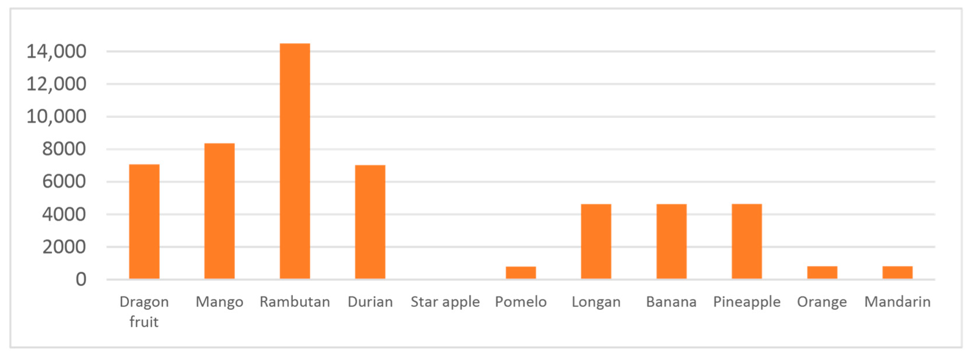
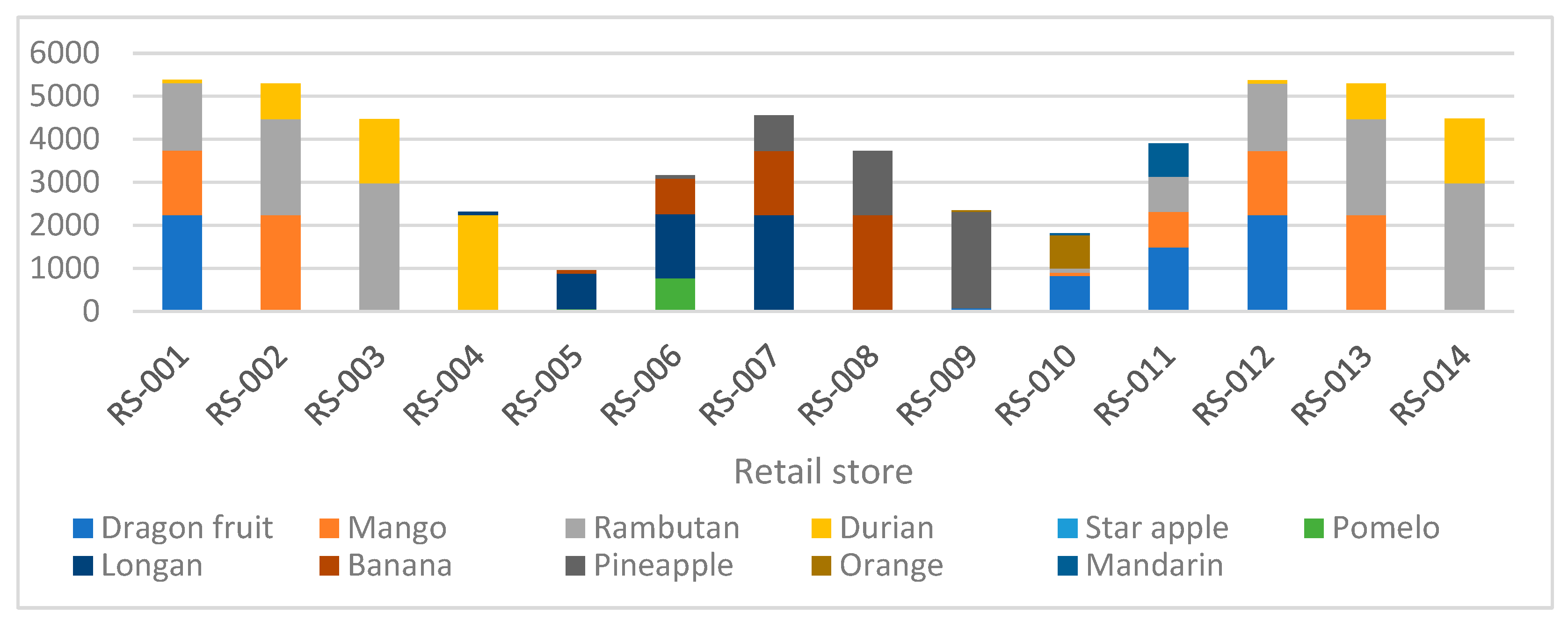
4.1. Case Study
4.2. Optimization Solutions
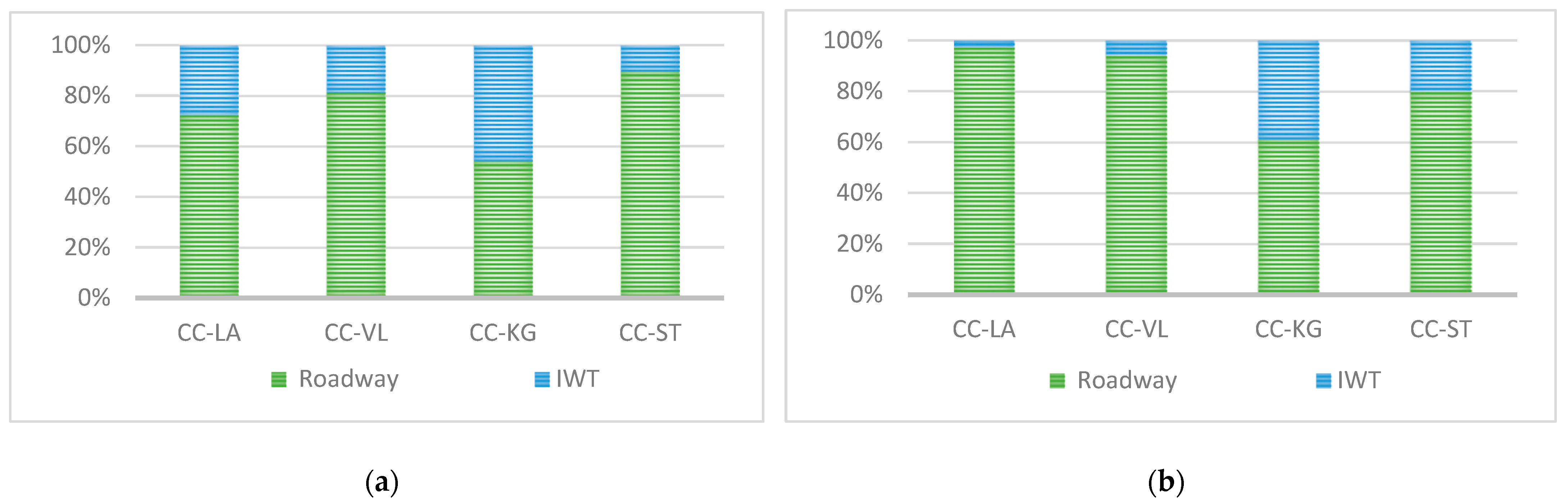
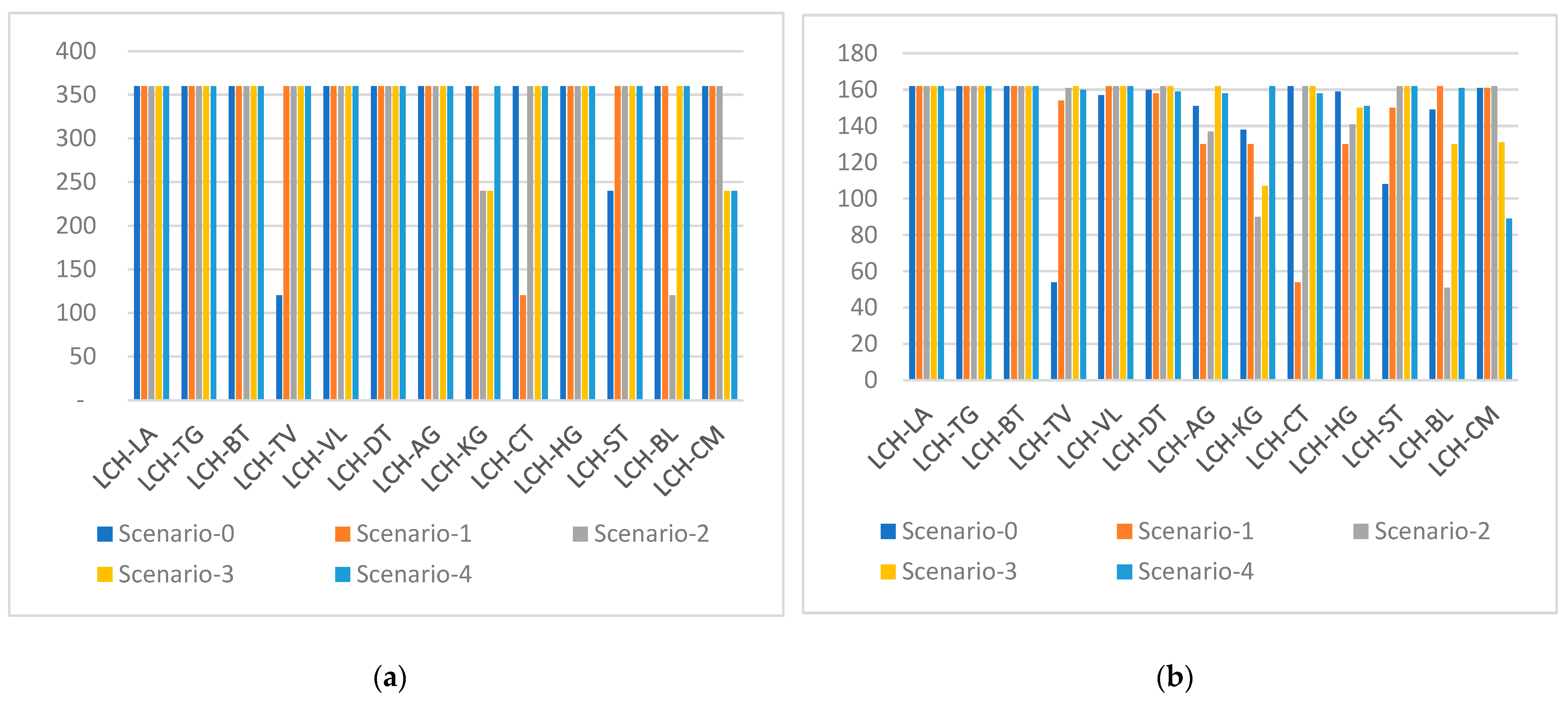
4.3. Experiments
5. Conclusions
Author Contributions
Funding
Acknowledgments
Conflicts of Interest
References
- Routray, W.; Orsat, V. Agricultural and Food Industry By-Products: Source of Bioactive Components for Functional Beverages. Nutr. Beverages 2019, 12, 543–589. [Google Scholar]
- Harris, J.; Nguyen, P.H.; Tran, L.M.; Huynh, P.N. Nutrition transition in Vietnam: Changing food supply, food prices, household expenditure, diet and nutrition outcomes. Food Secur. 2020, 12, 1141–1155. [Google Scholar] [CrossRef]
- González-Aguilar, G.; Robles-Sánchez, R.; Martínez-Téllez, M.; Olivas, G.; Alvarez-Parrilla, E.; de la Rosa, L. Bioactive compounds in fruits: Health benefits and effect of storage conditions. Stewart Postharvest Rev. 2008, 4, 1–10. [Google Scholar]
- Wang, C.-N.; Nguyen, M.N.; Le, A.L.; Tibo, H. A DEA Resampling Past-Present-Future Comparative Analysis of the Food and Beverage Industry: The Case Study on Thailand vs. Vietnam Math. 2020, 8, 1140. [Google Scholar] [CrossRef]
- Amorim, P.; Meyr, H.; Almeder, C.; Almada-Lobo, B. Managing perishability in production-distribution planning: A discussion and review. Flex. Serv. Manuf. J. 2011, 25, 389–413. [Google Scholar] [CrossRef]
- Osvald, A.; Stirn, L.Z. A vehicle routing algorithm for the distribution of fresh vegetables and similar perishable food. J. Food Eng. 2008, 85, 285–295. [Google Scholar] [CrossRef]
- Govindan, K.; Jafarian, A.; Khodaverdi, R.; Devika, K. Two-echelon multiple-vehicle location–routing problem with time windows for optimization of sustainable supply chain network of perishable food. Int. J. Prod. Econ. 2014, 152, 9–28. [Google Scholar] [CrossRef]
- Kannan, D.; Mina, H.; Nosrati-Abarghooee, S.; Khosrojerdi, G. Sustainable circular supplier selection: A novel hybrid approach. Sci. Total Environ. 2020, 722, 137936. [Google Scholar] [CrossRef] [PubMed]
- Koberg, E.; Longoni, A. A systematic review of sustainable supply chain management in global supply chains. J. Clean. Prod. 2019, 207, 1084–1098. [Google Scholar] [CrossRef]
- Wang, C.-N.; Ho, H.-X.; Luo, S.-H.; Lin, T.-F. An Integrated Approach to Evaluating and Selecting Green Logistics Providers for Sustainable Development. Sustainability 2017, 9, 218. [Google Scholar] [CrossRef] [Green Version]
- Wang, C.-N.; Nguyen, H.-K. Enhancing Urban Development Quality Based on the Results of Appraising Efficient Performance of Investors—A Case Study in Vietnam. Sustainability 2017, 9, 1397. [Google Scholar] [CrossRef] [Green Version]
- Sirilertsuwan, P.; Thomassey, S.; Zeng, X. A Strategic Location Decision-Making Approach for Multi-Tier Supply Chain Sustainability. Sustainability 2020, 12, 8340. [Google Scholar] [CrossRef]
- Hsu, H.-P.; Wang, C.-N. Resources Planning for Container Terminal in a Maritime Supply Chain Using Multiple Particle Swarms Optimization (MPSO). Mathematics 2020, 8, 764. [Google Scholar] [CrossRef]
- Eskandarpour, M.; Dejax, P.; Miemczyk, J.; Péton, O. Sustainable supply chain network design: An optimization-oriented review. Omega-Int. J. Manag. Sci. 2015, 54, 11–32. [Google Scholar] [CrossRef]
- Alizadeh Afrouzy, Z.; Nasseri, S.H.; Mahdavi, I.; Paydar, M.M. A fuzzy stochastic multi-objective optimization model to configure a supply chain considering new product development. Appl. Math. Model. 2016, 40, 7545–7570. [Google Scholar] [CrossRef]
- Elhedhli, S.; Merrick, R. Green supply chain network design to reduce carbon emissions. Transport. Res. D-Tr. E. 2012, 17, 370–379. [Google Scholar] [CrossRef]
- Zahir, S.; Sarker, R. Optimising multi-objective location decisions in a supply chain using an AHP-enhanced goal-programming model. Int. J. Logist. Syst. Manag. 2010, 6, 249–266. [Google Scholar] [CrossRef]
- Bahrampour, P.; Safari, M.; Taraghdari, M.B. Modeling Multi-Product Multi-Stage Supply Chain Network Design. Proc. Econ. Financ. 2016, 36, 70–80. [Google Scholar] [CrossRef] [Green Version]
- Farahani, R.Z.; Rezapour, S.; Drezner, T.; Fallah, S. Competitive supply chain network design: An overview of classifications, models, solution techniques and applications. Omega-Int. J. Manag. Sci. 2014, 45, 92–118. [Google Scholar] [CrossRef]
- Sarker, B.; Jamal, A.M.M.; Wang, S. Supply chain model for perishable products under inflation and permissible delay in payment. Comput. Oper. Res. 2000, 27, 59–75. [Google Scholar] [CrossRef]
- Blackburn, J.; Scudder, G. Supply Chain Strategies for Perishable Products: The Case of Fresh Produce. Prod. Oper. Manag. 2009, 18, 129–137. [Google Scholar] [CrossRef]
- Katsaliaki, K.; Mustafee, N.; Kumar, S. A game-based approach towards facilitating decision making for perishable products: An example of blood supply chain. Expert Syst. Appl. 2014, 41, 4043–4059. [Google Scholar] [CrossRef] [Green Version]
- Liu, L.; Liu, X.; Liu, G. The risk management of perishable supply chain based on coloured Petri Net modeling. Inf. Process. Agric. 2018, 5, 47–59. [Google Scholar] [CrossRef]
- Rong, A.; Akkerman, R.; Grunow, M. An optimization approach for managing fresh food quality throughout the supply chain. Int. J. Prod. Econ. 2011, 131, 421–429. [Google Scholar] [CrossRef]
- Etemadnia, H.; Goetz, S.J.; Canning, P.; Tavallali, M.S. Optimal wholesale facilities location within the fruit and vegetables supply chain with bimodal transportation options: An LP-MIP heuristic approach. Eur. J. Oper. Res. 2015, 244, 648–661. [Google Scholar] [CrossRef]
- de Keizer, M.; Akkerman, R.; Grunow, M.; Bloemhof, J.M.; Haijema, R.; van der Vorst, J.G.A.J. Logistics network design for perishable products with heterogeneous quality decay. Eur. J. Oper. Res. 2017, 262, 535–549. [Google Scholar] [CrossRef]
- Dutta, P.; Shrivastava, H. The design and planning of an integrated supply chain for perishable products under uncertainties. J. Model. Manag. 2020, 15, 1301–1337. [Google Scholar] [CrossRef]
- Bushuev, M.A.; Guiffrida, A.L. Optimal position of supply chain delivery window: Concepts and general conditions. Int. J. Prod. Econ. 2012, 137, 226–234. [Google Scholar] [CrossRef]
- Catalá, L.P.; Moreno, M.S.; Blanco, A.M.; Bandoni, J.A. A bi-objective optimization model for tactical planning in the pome fruit industry supply chain. Comput. Electron. Agric. 2016, 130, 128–141. [Google Scholar] [CrossRef]
- Razmi, J.; Kazerooni, M.P.; Sangari, M.S. Designing an integrated multi-echelon, multi-product and multi-period supply chain network with seasonal raw materials. Econ. Comput. Econ. Cybern. 2016, 50, 273–290. [Google Scholar]
- Yu, M.-C.; Wang, C.-N.; Ho, N.-N.-Y. A Grey Forecasting Approach for the Sustainability Performance of Logistics Companies. Sustainability 2016, 8, 866. [Google Scholar] [CrossRef] [Green Version]
- Musavi, M.; Bozorgi-Amiri, A. A multi-objective sustainable hub location-scheduling problem for perishable food supply chain. Comput. Ind. Eng. 2017, 113, 766–778. [Google Scholar] [CrossRef]
- Biuki, M.; Kazemi, A.; Alinezhad, A. An integrated location-routing-inventory model for sustainable design of a perishable products supply chain network. J. Clean. Prod. 2020, 260, 120842. [Google Scholar] [CrossRef]
- Wang, C.-N.; Dang, T.-T.; Le, T.Q.; Kewcharoenwong, P. Transportation Optimization Models for Intermodal Networks with Fuzzy Node Capacity, Detour Factor, and Vehicle Utilization Constraints. Mathematics 2020, 8, 2109. [Google Scholar] [CrossRef]
- Bortolini, M.; Faccio, M.; Gamberi, M.; Pilati, F. Multi-objective design of multi-modal fresh food distribution networks. Int. J. Logist. Syst. Manag. 2016, 24, 155. [Google Scholar] [CrossRef]
- Mohammed, A.; Wang, Q. The fuzzy multi-objective distribution planner for a green meat supply chain. Int. J. Prod. Econ. 2017, 184, 47–58. [Google Scholar] [CrossRef] [Green Version]
- Accorsi, R.; Gallo, A.; Manzini, R. A climate driven decision-support model for the distribution of perishable products. J. Clean. Prod. 2017, 165, 917–929. [Google Scholar] [CrossRef]
- Circular No.1648/QĐ-BNN-TT. July 2013. Available online: https://luatvietnam.vn/nong-nghiep/quyet-dinh-1648-qd-bnn-tt-bo-nong-nghiep-va-phat-trien-nong-thon-79898-d1.html (accessed on 30 June 2020).
- Blancas, L.C.; El-Hifnawi, M.B. Facilitating Trade through Competitive, Low-Carbon Transport: The Case for Vietnam’s Inland and Coastal Waterways; The World Bank: Washington, DC, USA, 2014. [Google Scholar]
- The Vietnam Household Living Standards Survey 2018. May 2020. Available online: https://www.gso.gov.vn/en/data-and-statistics/2020/05/result-of-the-vietnam-household-living-standards-survey-2018 (accessed on 27 July 2020).
- Rohmer, S.U.K.; Gerdessen, J.C.; Claassen, G.D.H. Sustainable supply chain design in the food system with dietary considerations: A multi-objective analysis. Eur. J. Oper. Res. 2019, 273, 1149–1164. [Google Scholar] [CrossRef]
- Jiang, Y.; Zhao, Y.; Dong, M.; Han, S. Sustainable Supply Chain Network Design with Carbon Footprint Consideration: A Case Study in China. Math. Prob. Eng. 2019, 2019, 1–19. [Google Scholar] [CrossRef]
- Yakavenka, V.; Mallidis, I.; Vlachos, D.; Iakovou, E.; Eleni, Z. Development of a multi-objective model for the design of sustainable supply chains: The case of perishable food products. Ann. Oper. Res. 2019, 294, 593–621. [Google Scholar] [CrossRef]
- Issues and Sustainable Development Orientation for Fruits in Mekong Delta. 2019. Available online: http://www.cuctrongtrot.gov.vn/TinTuc/Index/4433. (accessed on 20 December 2020).


| Set Notation | Set Indices | Description |
|---|---|---|
| N | Types of fruit | |
| G | Fruit gardens | |
| H | Potential local hubs | |
| C | Potential Crossdocking centers | |
| S | Fruit stores | |
| L | Facility scales | |
| M | m | Transportation modes |
| P | p | Objective functions |
| DM | d | Decision makers |
| Group | Notation | Parameters | Unit |
|---|---|---|---|
| 1 | Investment cost for local hub with facility scale | USD | |
| Investment cost for crossdocking center with facility scale | USD | ||
| Unit shipping cost with transportation mode | USD/ton-km | ||
| Annual labor cost for local hubs | USD/person | ||
| Annual labor cost for crossdocking centers | USD/person | ||
| 2 | Distance from fruit garden to local hub with transportation mode | Km | |
| Distance from local hub to crossdocking center with transportation mode | Km | ||
| Distance from crossdocking center to store with transportation mode | Km | ||
| Local hub designed capacity with facility scale | Ton/year | ||
| Crossdocking center designed capacity with facility scale | Ton/year | ||
| Designed crossdocking time for local hub | Hour/ton | ||
| Designed crossdocking time for crossdocking center | Hour/ton | ||
| Minimum capacity utilization for local hub | % | ||
| Minimum capacity utilization for crossdocking center | % | ||
| Maximum labor working hour for local hub | Hour | ||
| Maximum labor working hour for crossdocking center | Hour | ||
| Workforce production rate for local hub | Ton/hour | ||
| Workforce production rate for crossdocking center | Ton/hour | ||
| 3 | Vehicle payload with transportation mode | Ton | |
| Vehicle designed velocity with transportation mode | Km/hour | ||
| CO2 emission coefficient with transportation mode | Kg/ton-km | ||
| 4 | Annual supply capacity of fruit in fruit garden | Ton | |
| Annual demand of fruit in store | Ton | ||
| Available harvest date of fruit in fruit garden (Value 0~0:00 January 1st) | Hour | ||
| Maximum waiting time for harvest of fruit | Hour | ||
| Start date of time window for fruit in store (Value 0~0:00 January 1st) | Hour | ||
| End date of time window for fruit in store (Value 0~0:00 January 1st) | Hour |
| Notation | Decision Variables |
|---|---|
| The shipping quantity of fruit n from fruit garden to local hub with transportation mode | |
| The shipping quantity of fruit n from local hub to crossdocking center with transportation mode | |
| The shipping quantity of fruit n from crossdocking center to store with transportation mode | |
| Workforce level in local hub | |
| Workforce level in crossdocking center | |
| Early shipping time of fruit at store | |
| Late shipping time of fruit at store | |
| Latest harvest time of fruit in garden | |
| Latest arrival time of fruit in local hub | |
| Latest arrival time of fruit in crossdocking center | |
| Latest receiving time of fruit in store |
| Definition of Linguistic Term Scale | Numerical |
|---|---|
| Equally important | 1 |
| Weakly important | 3 |
| Essentially important | 5 |
| Very strongly important | 7 |
| Absolutely important | 9 |
| Intermediate value between two adjacent judgments | 2, 4, 5, 6 |
| No. | Major Fruit | Area (Hectares) |
|---|---|---|
| 1 | Dragon fruit | 7300 |
| 2 | Mango | 31,600 |
| 3 | Rambutan | 5500 |
| 4 | Durian | 10,500 |
| 5 | Star apple | 5000 |
| 6 | Pomelo | 25,000 |
| 7 | Longan | 26,300 |
| 8 | Banana | 21,400 |
| 9 | Pineapple | 21,000 |
| 10 | Orange | 26,250 |
| 11 | Mandarin | 5250 |
| Specifications | Roadway | Inland Waterway |
|---|---|---|
| Vehicle payload (ton) | 20 | 50 |
| Average velocity (Km/hour) | 50 | 10 |
| Emission (Kg CO2/ton-km) | 0.05654 | 0.15310 |
| Scale | Local Collection Hub | Crossdocking Center | ||
|---|---|---|---|---|
| Designed Capacity (Ton/Year) | Investment Cost (USD) | Designed Capacity (Ton/Year) | Investment Cost (USD) | |
| 1 | 120,000 | 96,750 | 1,200,000 | 1,161,000 |
| 2 | 240,000 | 245,100 | 1,920,000 | 1,935,000 |
| 3 | 360,000 | 335,400 | 2,400,000 | 2,128,500 |
| Objective Value | ||||
|---|---|---|---|---|
| Total cost (USD) | 66,903,479 | 110,975,279 | 290,631,549 | 111,662,385 |
| Total delivery time (hour) | 1,098,291 | 491,200 | 3,213,428 | 491,492 |
| On-time delivery factor (hour) | 86,386 | 86,147 | 52,877 | 86,160 |
| Transportation emissions (Kg CO2) | 83,750,964 | 28,196,007 | 223,276,145 | 28,121,281 |
| Expert | Weight | Consistency Ratio (%) | |||
|---|---|---|---|---|---|
| 1 | 0.3645 | 0.1242 | 0.2336 | 0.2777 | 1.70 |
| 2 | 0.5438 | 0.2243 | 0.1030 | 0.1289 | 5.09 |
| 3 | 0.2752 | 0.4671 | 0.1062 | 0.1515 | 3.60 |
| 4 | 0.4053 | 0.1321 | 0.0867 | 0.3759 | 1.71 |
| 5 | 0.3359 | 0.3754 | 0.1898 | 0.0989 | 4.42 |
| 6 | 0.5443 | 0.1373 | 0.2424 | 0.0760 | 6.98 |
| 7 | 0.3935 | 0.2337 | 0.0746 | 0.2982 | 5.71 |
| 8 | 0.1766 | 0.2460 | 0.2956 | 0.2818 | 6.86 |
| 9 | 0.4444 | 0.2416 | 0.2109 | 0.1031 | 6.40 |
| 10 | 0.4718 | 0.2124 | 0.2174 | 0.0984 | 2.32 |
| 11 | 0.0930 | 0.5249 | 0.2388 | 0.1433 | 3.25 |
| 12 | 0.2044 | 0.5844 | 0.1124 | 0.0988 | 5.40 |
| 13 | 0.1345 | 0.4811 | 0.2586 | 0.1258 | 4.39 |
| 14 | 0.3302 | 0.0934 | 0.2062 | 0.3702 | 7.42 |
| 15 | 0.3399 | 0.0935 | 0.2268 | 0.3398 | 4.60 |
| 16 | 0.4409 | 0.1392 | 0.1638 | 0.2562 | 6.97 |
| 17 | 0.1560 | 0.2854 | 0.4396 | 0.1190 | 5.37 |
| 18 | 0.3704 | 0.1464 | 0.2780 | 0.2052 | 7.66 |
| 19 | 0.4527 | 0.0990 | 0.1708 | 0.2775 | 8.26 |
| 20 | 0.3319 | 0.1257 | 0.2348 | 0.3076 | 3.01 |
| Objective | ||
|---|---|---|
| Total cost (USD) | 125,120,510 | |
| Investment cost | 8,675,250 | |
| Labor cost | 21,023,990 | |
| Transportation cost | 95,421,270 | |
| Total delivery time (hour) | 606,547 | |
| On-time delivery factor (hour) | 53,101 | |
| Transportation emissions (Kg CO2) | 35,547,459 | |
| Scenario | Weight | |||
|---|---|---|---|---|
| Scenario-0 | 0.303 | 0.215 | 0.191 | 0.291 |
| Scenario-1 | 0.250 | 0.250 | 0.250 | 0.250 |
| Scenario-2 | 0.200 | 0.500 | 0.150 | 0.150 |
| Scenario-3 | 0.150 | 0.150 | 0.500 | 0.200 |
| Scenario-4 | 0.100 | 0.100 | 0.300 | 0.500 |
| Objective | Scenario-1 | Scenario-2 | Scenario-3 | Scenario-4 |
|---|---|---|---|---|
| Total cost (USD) | −3.6677% | −5.1133% | −4.0346% | −5.6211% |
| Total delivery time (hour) | 1.3177% | 2.3243% | 7.6035% | 7.2972% |
| On-time delivery factor (hour) | −0.4670% | −0.0810% | 0.0000% | 0.0075% |
| Transportation emissions (Kg CO2) | 3.5895% | 5.5664% | 10.1131% | 10.5422% |
Publisher’s Note: MDPI stays neutral with regard to jurisdictional claims in published maps and institutional affiliations. |
© 2021 by the authors. Licensee MDPI, Basel, Switzerland. This article is an open access article distributed under the terms and conditions of the Creative Commons Attribution (CC BY) license (http://creativecommons.org/licenses/by/4.0/).
Share and Cite
Wang, C.-N.; Nhieu, N.-L.; Chung, Y.-C.; Pham, H.-T. Multi-Objective Optimization Models for Sustainable Perishable Intermodal Multi-Product Networks with Delivery Time Window. Mathematics 2021, 9, 379. https://doi.org/10.3390/math9040379
Wang C-N, Nhieu N-L, Chung Y-C, Pham H-T. Multi-Objective Optimization Models for Sustainable Perishable Intermodal Multi-Product Networks with Delivery Time Window. Mathematics. 2021; 9(4):379. https://doi.org/10.3390/math9040379
Chicago/Turabian StyleWang, Chia-Nan, Nhat-Luong Nhieu, Yu-Chi Chung, and Huynh-Tram Pham. 2021. "Multi-Objective Optimization Models for Sustainable Perishable Intermodal Multi-Product Networks with Delivery Time Window" Mathematics 9, no. 4: 379. https://doi.org/10.3390/math9040379