Optimisation of Time-Varying Asset Pricing Models with Penetration of Value at Risk and Expected Shortfall

Abstract

This study aims to apply value at risk (VaR) and expected shortfall (ES) as time-varying systematic and idiosyncratic risk factors to address the downside risk anomaly of various asset pricing models currently existing in the Pakistan stock exchange. The study analyses the significance of high minus low VaR and ES portfolios as a systematic risk factor in one factor, three-factor, and five-factor asset pricing model. Furthermore, the study introduced the six-factor model, deploying VaR and ES as the idiosyncratic risk factor. The theoretical and empirical alteration of traditional asset pricing models is the study’s contributions. This study reported a strong positive relationship of traditional market beta, value at risk, and expected shortfall. Market beta pertains its superiority in estimating the time-varying stock returns. Furthermore, value at risk and expected shortfall strengthen the effects of traditional beta impact on stock returns, signifying the proposed six-factor asset pricing model. Investment and profitability factors are redundant in conventional asset pricing models.

1. Introduction

The current study elaborates the comparison of various risk factors and signifies the sensitivity of returns towards these risk factors. There are two types of risk; one is the systematic risk, which cannot be avoided. The other is the idiosyncratic risk that can be avoided or reduced [1]. The Capital Asset Pricing Model (CAPM) introduced market beta as the systematic risk factor. Market beta provides the sensitivity of security returns towards well-diversified portfolio returns. Idiosyncratic risk is generated from firm-specific factors, and it can be evaded by changing the investment strategy or diversification. Value at Risk (VaR) and Expected Shortfall (ES) are the risk factors related to the worst expected losses and systematically measure risk [2,3]. This study applies VaR and ES as both systematic and idiosyncratic risk factors and signifies the optimum risk-return trade-off.

The risk is the asymmetric position related to the loss [4]. The global financial crisis (Black Monday of 19 October 1987 when S&P 500 fell more than 20% in one day, the hedge fund crises of 1998, Asian financial crises of 1997–1998, the global financial crises of 2007) demanded the need for practical and authentic risk mitigation tools in securities markets. The formation of the exact risk management mechanism has always been a challenge for institutions and regulators. In the real world, the investments that contain high returns are connected with large deviations. Investors looking for high returns have to bear a high probability of risk [5]. The problems that investors face are calculating the expected value of investment and measurement of risk. Investors can reduce their risk by diversification [6]. VaR and ES are tools for estimation accuracy. VaR was extensively used as the internal risk measurement and backtesting tool by BASEL II accord, but ES replaced it in 2016 by BASEL III [7]. VaR is a quantile-based method, and ES, also known as conditional value at risk (CVaR), is tail risk measure, and both are the representation of extreme value theory. These risk measurement approaches are well known to identify the banking sector’s capital requirement to the market systematic risk. We can deploy these methods to develop the asset pricing model, producing better estimation for stock returns.

2. Review of Literature

Sharpe [8], Lintner [9], and Black [10] introduced the foundation of the effect of systematic risk and return correlation. They suggested the CAPM beta as the systematic risk factor to predict stock returns’ time variation. With the passage of time, the market introduced the anomalies related to the CAPM model. The literature presents specific idiosyncratic risk factors that can alter the stock returns differently, and investors can diversify to reduce risk by using these factors [11]. 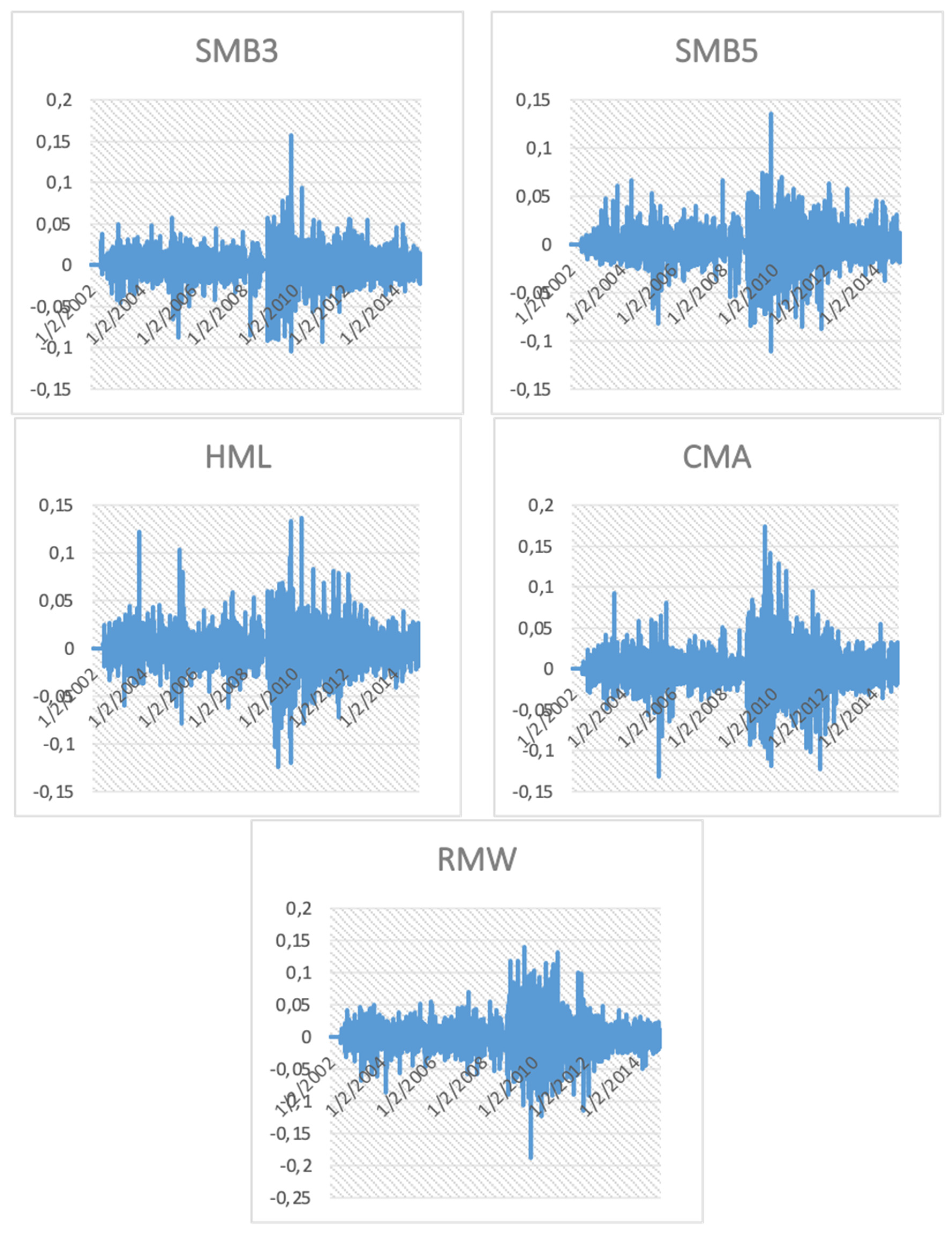Fama and French’s [12] three-factor model concluded that small-size stocks could outperform large-sized stocks and value stocks have more returns than growth stocks. They proxied size factor with SMB factor, i.e., small minus big stocks and value factor with HML, i.e., value stocks minus growth stocks.

Fama et al. [13] increased the three-factor model to the five-factor model by introducing investment and profitability factors. They indicated that stocks with robust profitability had more returns than stocks with weak profitability. Further, they showed that stocks outperform the conservative stocks with an aggressive investment strategy. Nhu significantly implemented the Fama and French [14] five-factor model in Vietnam. Cakici [15] signified the five-factor effect in European, North American, and other developed financial markets. They reported the irrelevant impact of investment and profitability factor in Asian and Japanese markets. Kubota et al. [16] reported t.3xhe redundancy of the Japanese stock market’s investment factor. Huang [17] focused on the Chinese stock market and compared the traditional Sharpe [8], Lintner [9] single-factor model with Fama and French [18] three-factor and Fama et al. [19] five-factor model. They reported the superiority of the five-factor model in the Chinese stock market. They also reported the significance of size factor, and weaker effect of value factor on stock returns. Our study adds to the body of knowledge by adding the VaR and ES as the model’s risk factors. We have deployed VaR and ES as the systematic risk factor, but We have also introduced VaR and ES as the sixth idiosyncratic risk factor. We have introduced VaR and ES in the six-factor model as the idiosyncratic market risk factor. In line with our study, Haque and Nasir [20] introduced VaR and ES as the systematic risk control mechanism, but they used cross-sectional analysis and did not introduce a six-factor model with VaR and ES the idiosyncratic market risk factors.

3. Materials and Methods

The population of the study is companies that are listed on the Pakistan Stock Exchange PSX. The data of 527 companies are taken as a sample, listed on the PSX from 1998 to 2015. Maditinos et al. [21] did not take financial institutions as a sample because of the high leverage in these sectors. The study has not included financial institutions. Researchers have cut the bankrupted and delisted companies. After adjusting the companies’ data, the first step is to find the annual data. The log of market equity (lnME), which is collected annually, to be used as the proxy for the size factor, book-to-market equity (BM) for value factor, operating profitability (OP) as a proxy for the profitability factor and change in the fixed asset is taken as the proxy for the investment factor (INV) [22]. The researchers have found annual VaR and ES for each company at 95% and 99% level of significance from the daily data. Following are the distinguished calculations of risk factors. From annual data time-varying factors are defined and measured.

3.1. Size Factor

This study aims to analyse the time-series effect of risk factors on stock returns. The researchers have arranged data according to annual data. The size factor represents a portfolio of stocks with low market equity minus the stock with high market equity abbreviated as small minus big stocks (SMB). The study uses annual data to form the portfolios and calculates average stock returns of small equities and big equities for the three-factor model [23]. The size factor calculation is different from the three-factor model’s size factor for the five-factor model, as represented by Fama et al. [13,22]. The average value of high-value stock and low-value stocks is required for three-factor and five-factor model average returns of high book-to-market and low book-to-market ratio, increased investment and low investment, and average returns of high operating profits and low operating profits are required. The equations for three-factor SMB and five-factor SMB are given below.

This study provides both the three-factor model (Fama et al, 1993, 1996) and the five-factor model [13]. Different portfolios of market equity are formed separately for three-factor and five-factor models.

SMB for three factors:

$$SM{B}_t= \frac{\left(small value+small neutral+small growth\right)}{3}+\frac{\left(big value+big neutral+big growth\right)}{3}$$

(1)

Portfolios are formed to find the time-series SMB factor. Small, neutral, and big stocks are found for each factor, i.e., book-to-market, investment and profitability, and new SMB is formed. The equations for calculations of SMB portfolio for the five-factor model are given below:

$$SM{B}_t\left(BM\right)= \frac{\left(small value+small neutral+small growth\right)}{3}+\frac{\left(big value+big neutral+big growth\right)}{3}$$

(2)

$$SM{B}_t\left(OP\right)= \frac{\left(small robust+small neutral+small weak\right)}{3}+\frac{\left(big robust+big neutral+big weak\right)}{3}$$

(3)

$$\begin{array}{c}SM{B}_t\left(INV\right)= \left(small Conservative+small neutral+small aggressive\right)/3+\\ \left(big Conservative+bmall neutral+bmall aggressive\right)/3,\end{array}$$

(4)

$$SM{B}_t=\frac{SM{B}_t\left(BM\right)+SM{B}_t\left(OP\right)+SM{B}_t\left(INV\right)}{3}$$

(5)

SMB for three-factor and five-factor are used for time-series estimation.

3.2. Value Factor

The value factor is calculated from the annual data of 527 manufacturing companies. We have dropped negative book-to-market ratio firms from the analysis because of high financial distress [24]. Yearly data of book-to-market ratio is considered the single point in time value factor used for cross-sectional analysis. The time-series analysis of the high minus low book to the market ratio (HML) is calculated from the following equation.

$$HM{L}_t= \frac{\left(small value+big value\right)}{2}+\frac{\left(small growth+big growth\right)}{2}$$

(6)

3.3. Profitability Factor

A previous year firm’s operating profitability is used to estimate the current year excess stock returns for cross-sectional analysis. The formula for operating profitability for annual data is given below:

$$O{P}_t=\frac{Earning before interest and texes \left(EBIT\right)}{Market equit{y}_{t-1}}$$

(7)

Further annual firms’ profitability data is arranged according to firms with robust profitability and weak profitability, and is segregated further into small robust and big robust profitability firms than firms with small weak and big weak profitability. Average returns of stocks are calculated for each portfolio, then with the help of the following formula, RMW firms are calculated [22]:

$$RM{W}_t= \frac{\left(small robust+big robust\right)}{2}+\frac{\left(small weak+big weak\right)}{2}$$

(8)

3.4. Investment Factor

We calculate the investment factor by undertaking the investment in total assets. If assets increased from the past year, the company is investing. The annual investment factor estimates the change in the previous year (t − 1) total assets from the last two years (t − 2) total assets. The equation is given below:

$$IN{V}_{it}=\frac{T{A}_{i,t-1} - T{A}_{i,t-2}}{T{A}_{t-2}}$$

(9)

where INV is the investment factor of the current year, and TA is the total asset.

The annual value of each year’s investment factor from 2000 to 2015 is calculated from the above equation. According to yearly investment data, firms are arranged according to conservative stocks, with lower investment in assets and aggressive stocks, who invest more rigorously. Different firms’ data is organized according to small conservative stocks and big conservative stocks, then small aggressive stocks and big aggressive stocks. Average returns of each portfolio of stocks are calculated, and from the following equation, the CMA factor, i.e., conservative minus aggressive stocks are estimated [25].

$$CM{A}_t= \frac{\left(small conservative+big conservative\right)}{2}+\frac{\left(small agressive+big agressive\right)}{2}$$

(10)

3.5. Value at Risk and Expected Shortfall

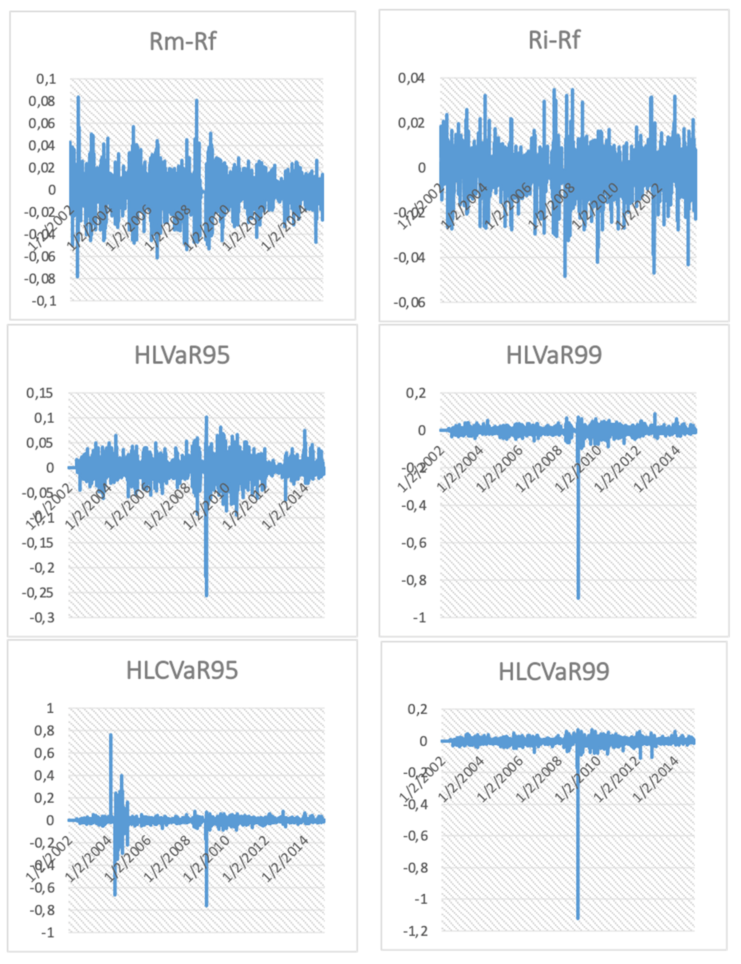
VaR projects the worst expected loss and ES represents the worst expected losses. The topic is primary in its nature for Pakistan’s financial market setup. The arrangement and development of VaR and ES in Pakistan is a challenge. The researcher has to go through time-consuming and lengthy data arrangement procedure to find high low VaR (HLVaR) and high minus low CVaR (HLCVaR). First, daily data of 527 firms listed on the PSX is collected from the Pakistan Stock Exchange. The dynamics of Pakistan play a role in the development of the models. Each firm’s data is compiled separately from the Pakistan Stock Exchange. Information is arranged in an Excel file, and each firm has been assigned a unique serial number. Continuously compounded returns are calculated from the daily prices of each stock. Year-wise historical VaR and ES are computed for each stock at 95% and 99% confidence levels. Each year, firms are arranged according to VaR and ES value and then placed according to first and fourth quartiles from highest VaR and ES value firms to the lowest VaR and ES value firms. First quartile firms considered high VaR and high ES or CVaR stocks and the fourth quartile is considered low VaR and low ES stocks at 95% and 99% confidence level. Historical VaR estimates are used because of the abnormal distribution of Pakistani stocks. Average returns of high and low VaR and CVaR stocks are computed. At 1% and 5% level of significance, the difference between the average returns of high VaR and ES stock portfolios and low VaR and ES portfolios provide high low VaR (HLVaR) and high low CVaR (HLCVaR) portfolios.

3.6. Time-Series Variation in Stock Returns

Equation (11) is used to measure the time-series effect of market risk on stock excess return. This study derives the new variable in the regression analysis, i.e., HLVaR to capture the portfolio’s time-series effect. This variable indicates the returns representing the securities with high VaR values minus the average stock returns with low VaR values. Further, the study has computed the time-series regression analysis using the following equation.

(Ri − Rf)t = γt + β1HLVaRt,α + εt.

(11)

VaR has been calculated at 95% and 99% confidence levels; the confidence levels are supported by Basel II committee of banking supervision. VaR is calculated with the normal distribution assumption, following the central limit theorem and significant one period ahead time horizon is assumed. Equation (12) uses HLCVaR at both 95% and 99% level of confidence. The estimate is calculated by differentiating average returns of high CVaR stock from average low CVaR stocks’ average returns.

(Ri − Rf)_t = γ_t + β₁HLCVaR_α,t + ε_t

(12)

Further, the explanatory power and significance of VaR and CAPM are tested with the inclusion of the idiosyncratic variables that are proposed by Benz [26], Basu [27], and Fama et al. [13,18].

Fama et al. [17] suggested size factor irregularity in the CAPM model. They stated that small size stocks generated more returns, which was also favored by Benz [26]. They suggested that returns of value stocks were more than growth stocks, and with the inclusion of these variables, the CAPM beta gave a more accurate explanation of stock returns. To check the explanatory power of these variables Equation (13) is formed:

(Ri−Rf)_t = α_t+ β₁(Rm − Rf)_t + β₂SMB_t + β₃HML_t + ε_t.

(13)

Further, this study contributes to the representation of the three-factor model using VaR and ES as the controlling mechanism of systematic risk and includes the idiosyncratic factors proposed by Fama et al. [13]. VaR is measured by an equally weighted moving average, and average extreme values are used to find ES or CVaR. The study completes its objective by providing the explanatory difference among CAPM, VaR, and ES:

(Ri − Rf)_t = α_t + β₁HLVaR_t + β₂SMB_t + β₃HML_t + ε_t

(14)

(Ri − Rf)_t = α_t + β₁HLCVAR_t + β₂SMB_t + β₃HML_t + ε_t

(15)

The Fama and French [13] five-factor model is analyzed by adding two idiosyncratic factors, i.e., robust minus weak profitability (RMW) and conservative minus aggressive investment (CMA). The five-factor model has used CAPM, VaR, and CVaR as the systematic risk factor for evaluating the estimation difference.

(Ri − Rf)_t = α_t + β₁(Rm − Rf)_t + β₂SMB_t + β₃HML_t + β₄RMW_t + β₅CMA_t + ε_t,

(16)

(Ri − Rf)_t = α_t + β₁HLVaRt + β₂SMB_t + β₃HML_t + β₄RMW_t + β₅CMA_t + ε_t,

(17)

(Ri − Rf)_t = α_t + β₁HLCVaR_t + β₂SMB_t + β₃HML_t + β₄RMW_t + β₅CMA_t + ε_t.

(18)

Equation (16) represents the Fama, and French five-factor model and the two other models are tested based on VaR and ES in Equations (17) and (18).

The study analyses the explanatory power of systematic risk and idiosyncratic risk factors. This study presents the six-factor model in which the question is whether downside risk, VaR, can be used as the systematic risk factor or idiosyncratic risk factor. If the effect of market beta reduced with VaR’s inclusion at 95% and 99% confidence levels, then VaR is alternating the impact of market beta. If the effect of market beta gets superior, then VaR is proving to be the significant idiosyncratic risk factor.

(Ri − Rf)_t = α_t + β₁(Rm − Rf)_t + β₂HLVaR_t + β₃SMB_t + β₄HML_t+ β₅RMW_t + β₆CMA_t + ε_t.

(19)

The above model uses market beta and high minus low VaR as the systematic risk factors and size, value, investment and profitability are used as the idiosyncratic risk factor estimating the excess stock returns.

(Ri − Rf)_t = α_t+ β₁(Rm − Rf)_t + β₂HLCVaR_t + β₃SMB_t + β₄HML_t+ β₅RMW_t + β₆CMA_t + ε_t.

(20)

Equation (20) is similar to Equation (19), but the difference is that the study excludes VaR and includes ES or CVaR. The equation estimates the significance of systematic risk and idiosyncratic risk using systematic and the rest of the model’s idiosyncratic risk factors.

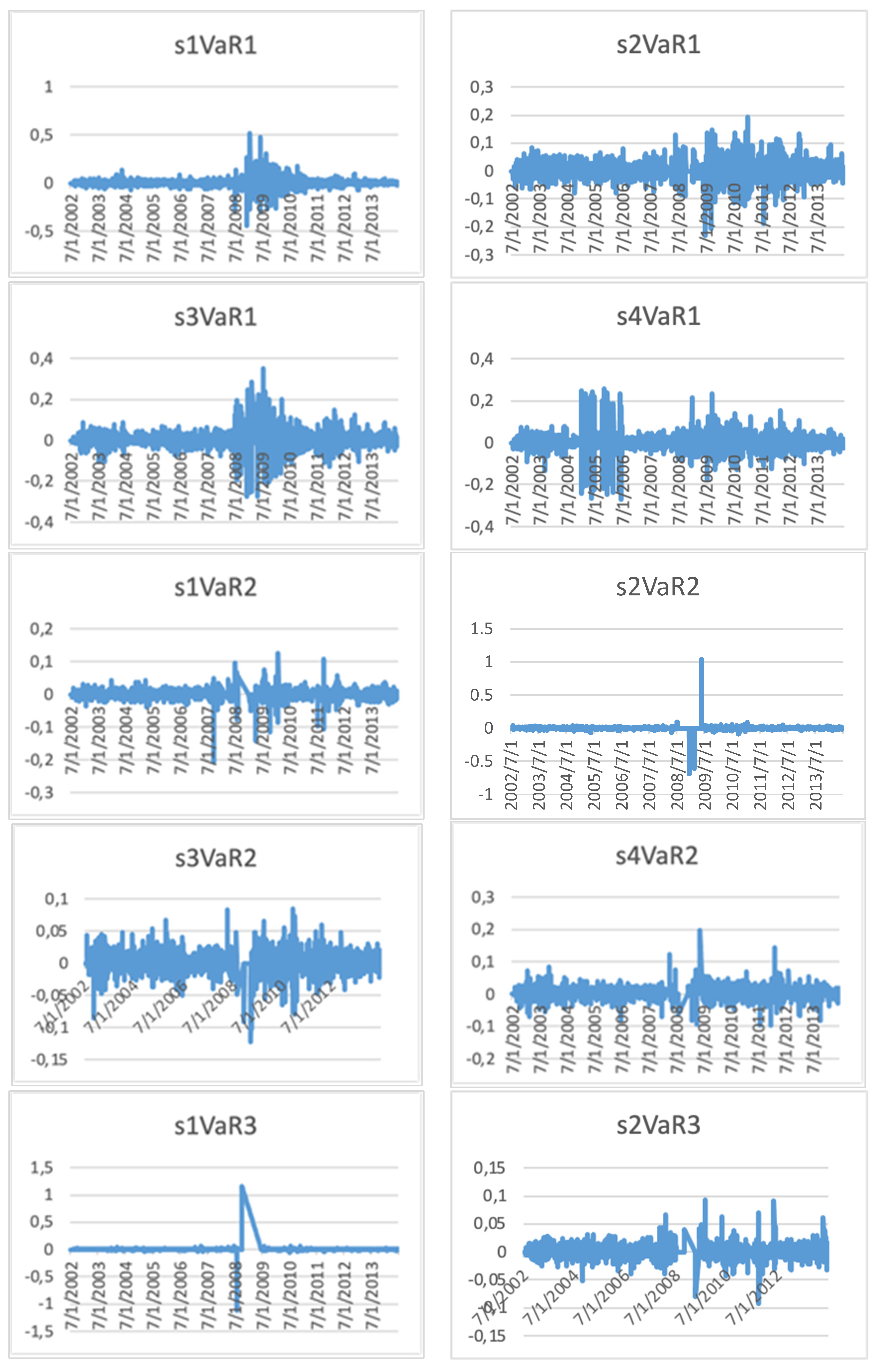
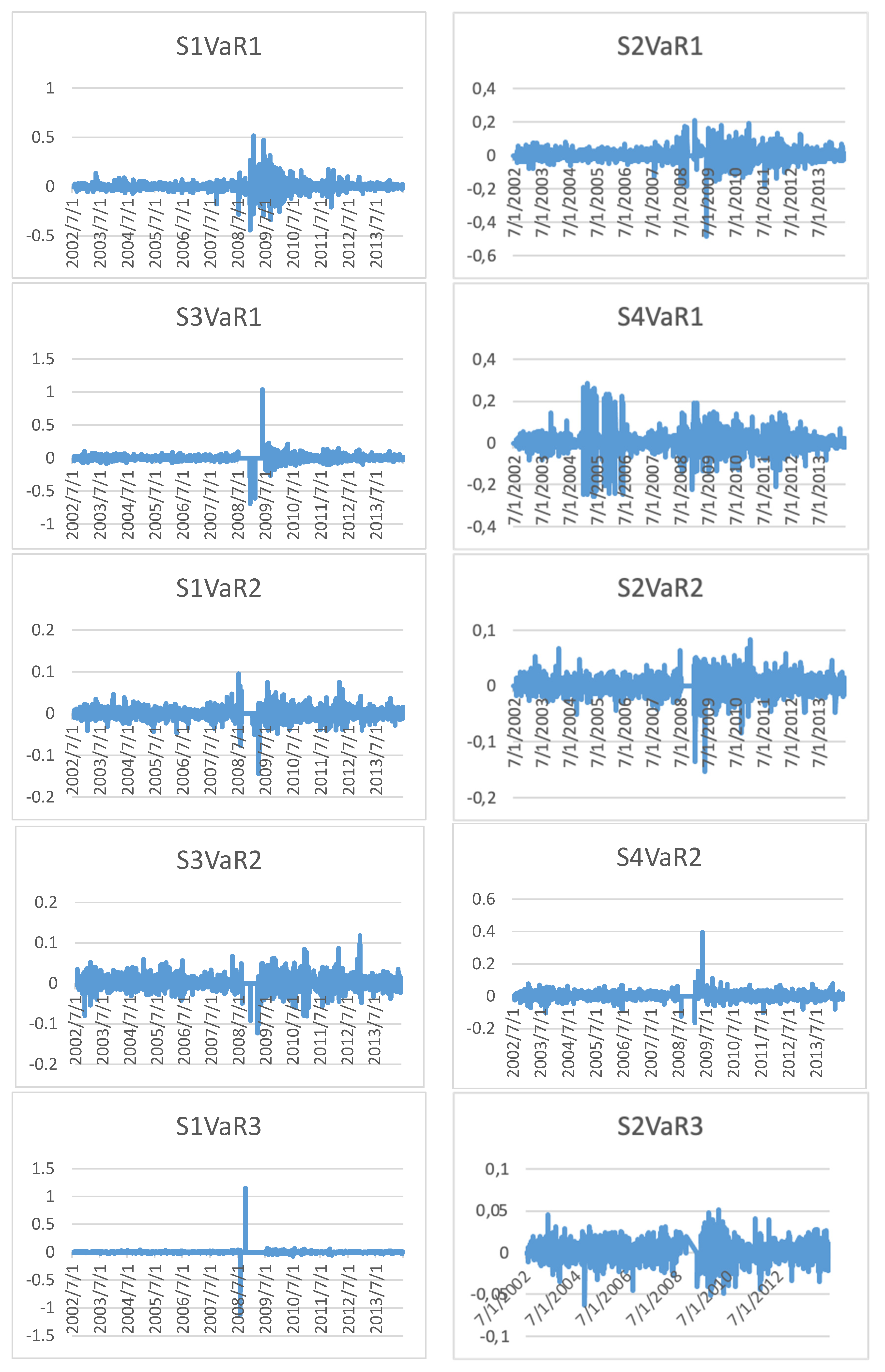
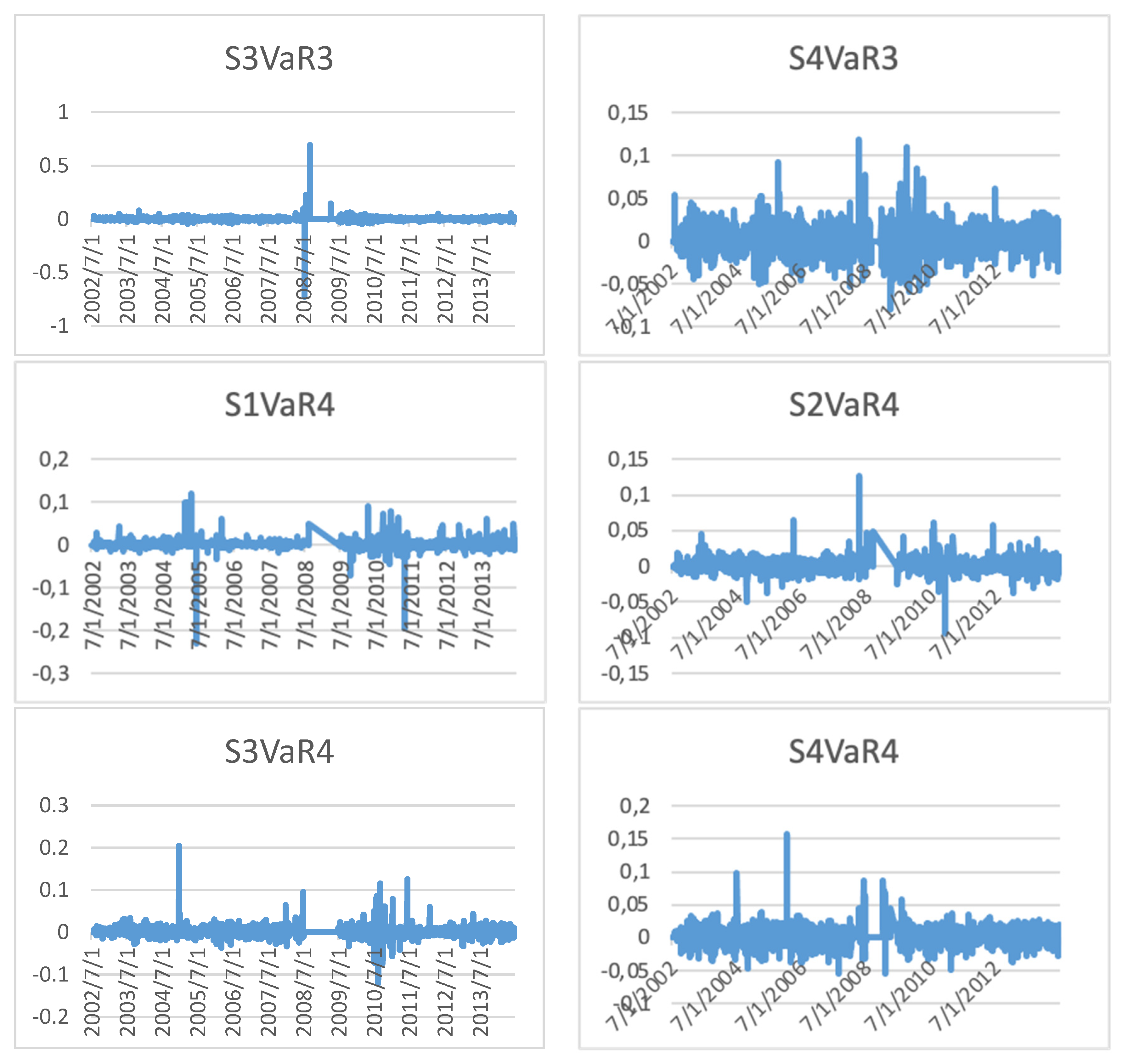
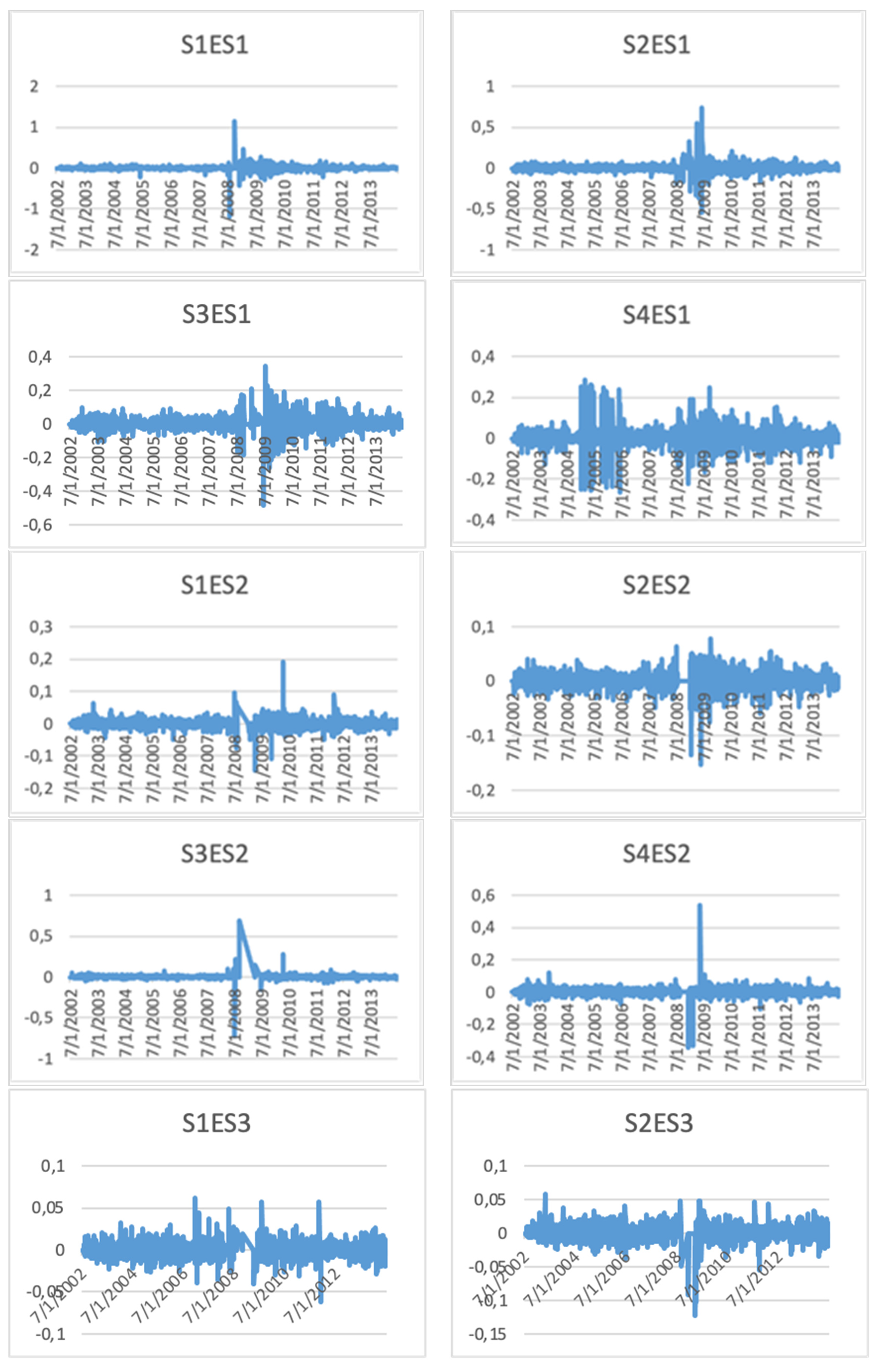
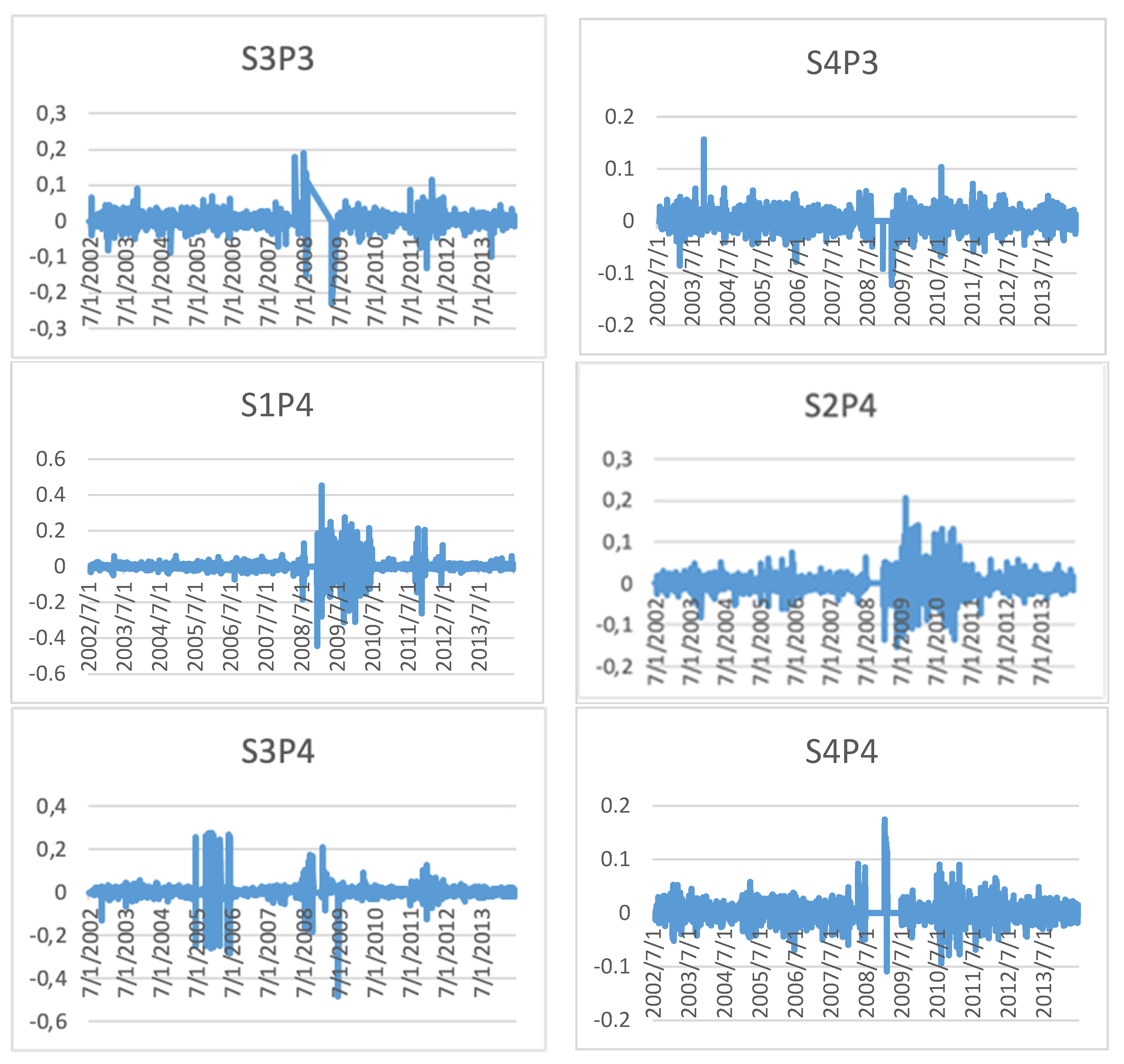
3.7. Time Varying Portfolio Structures

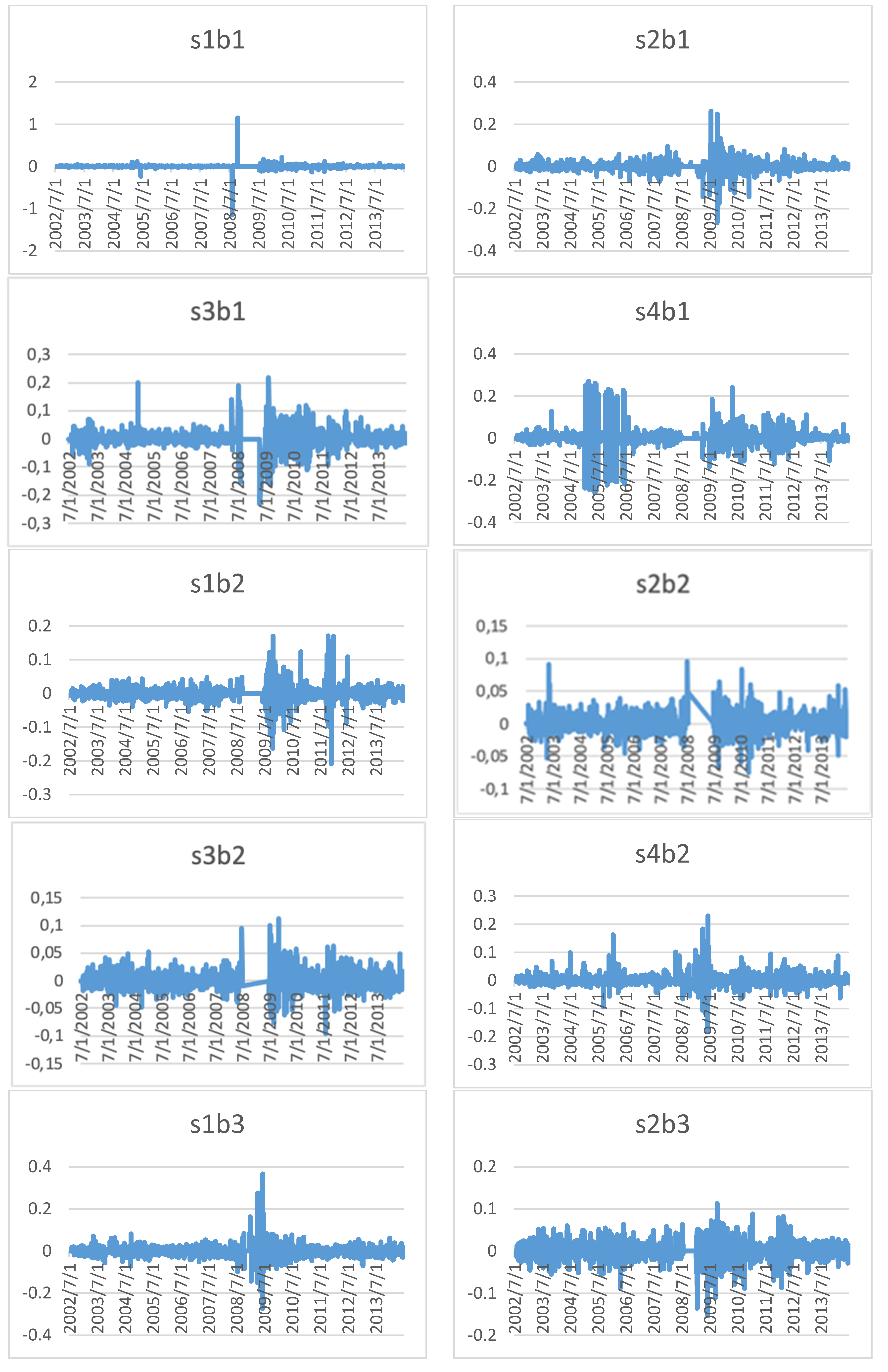
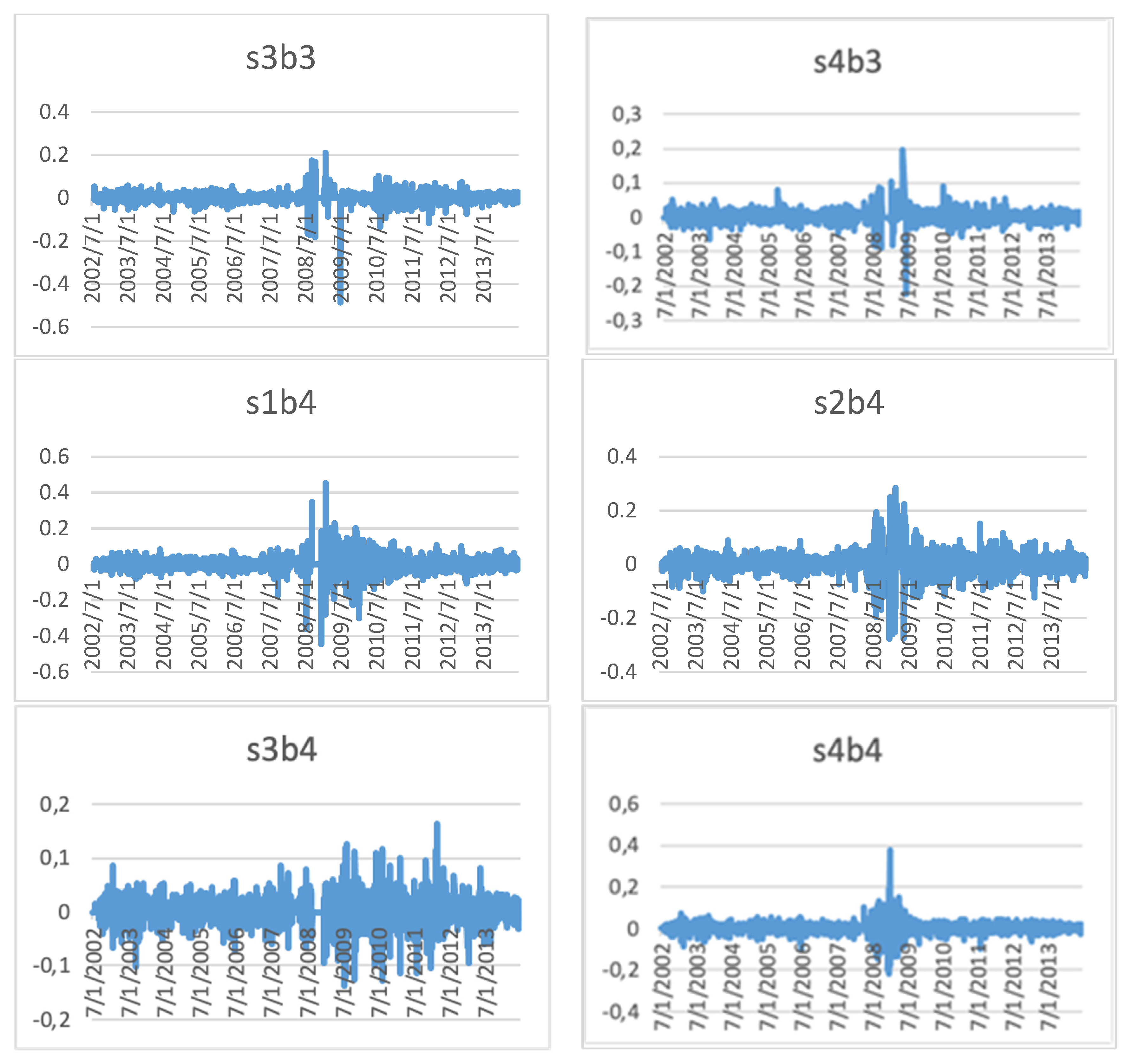
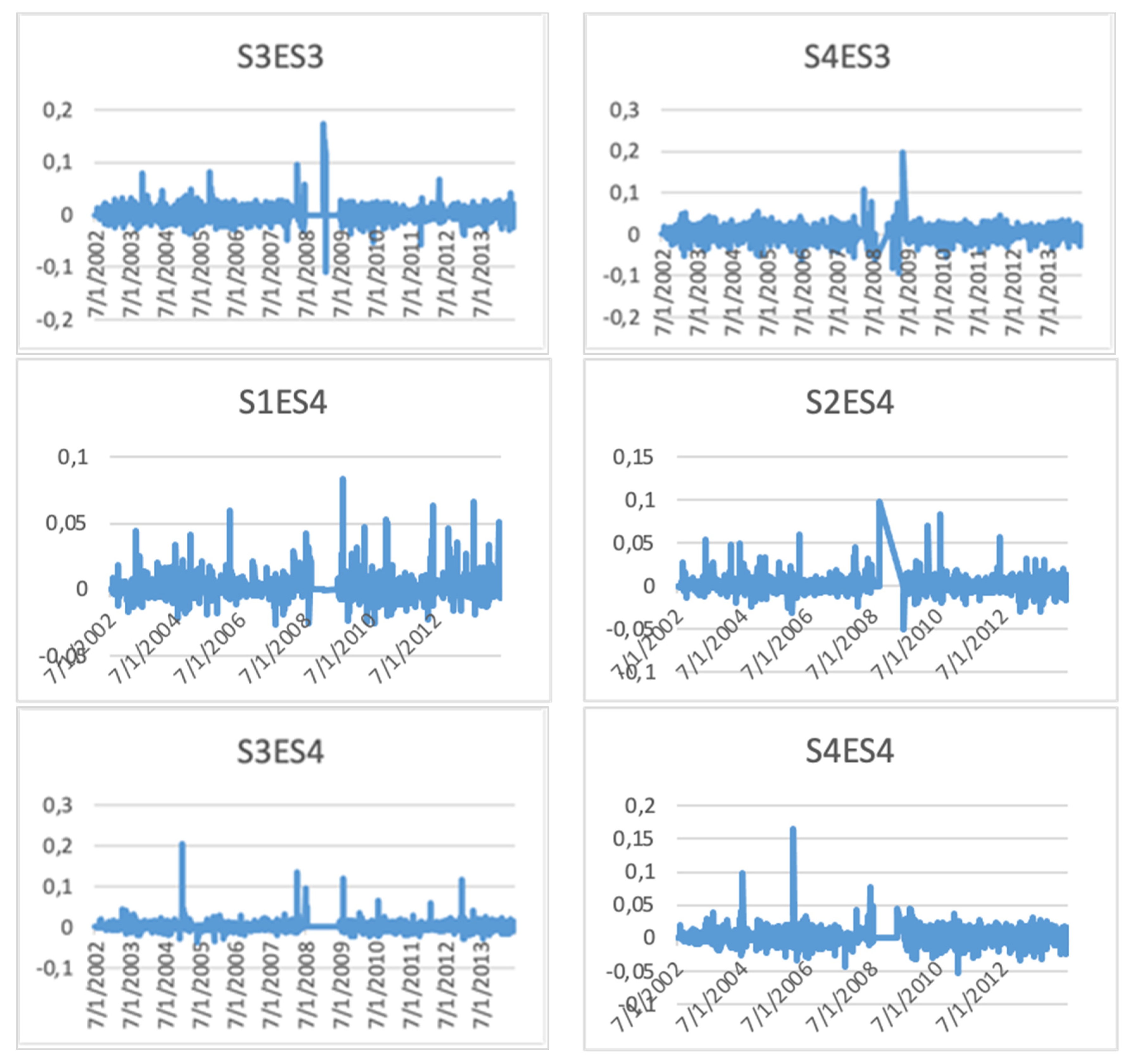
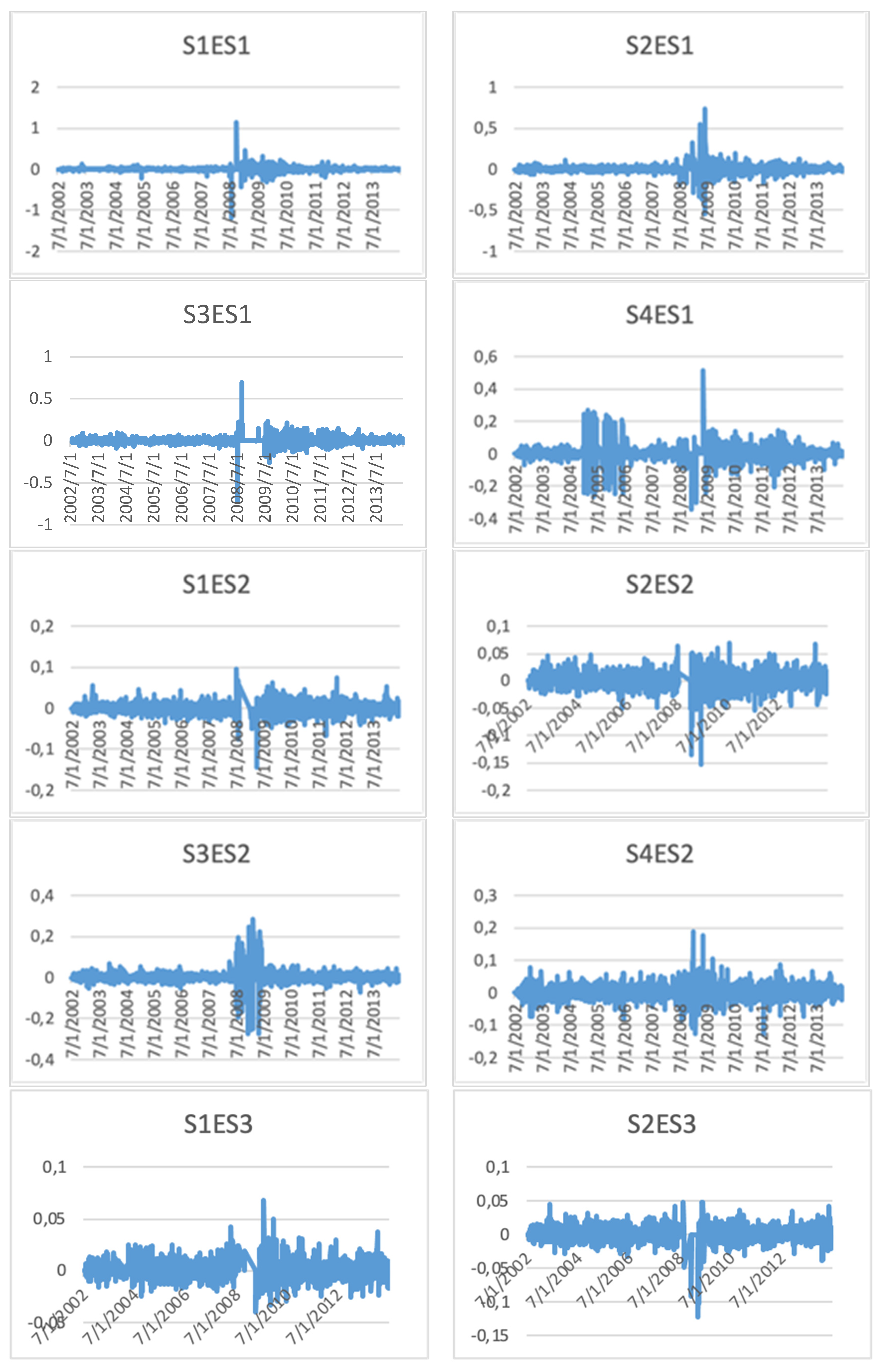
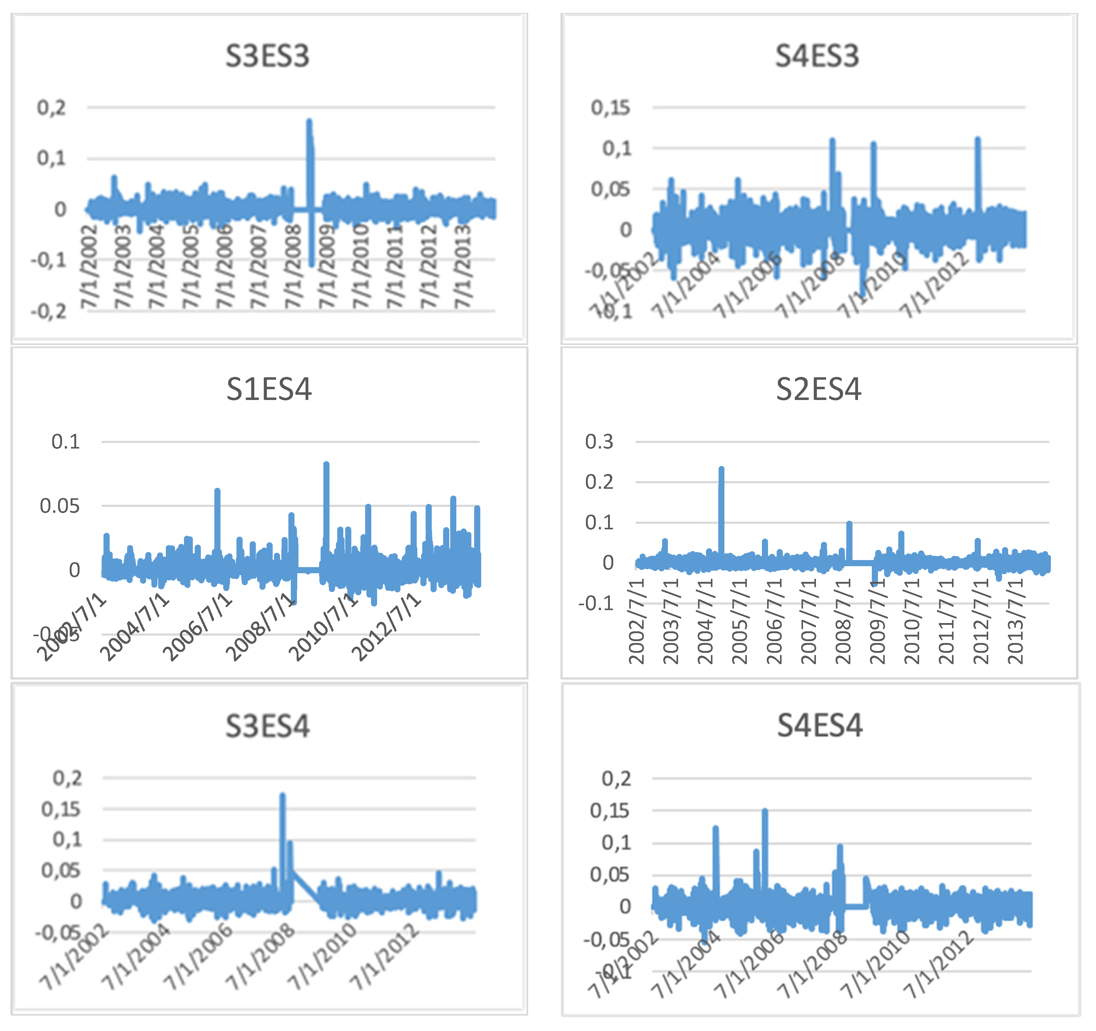
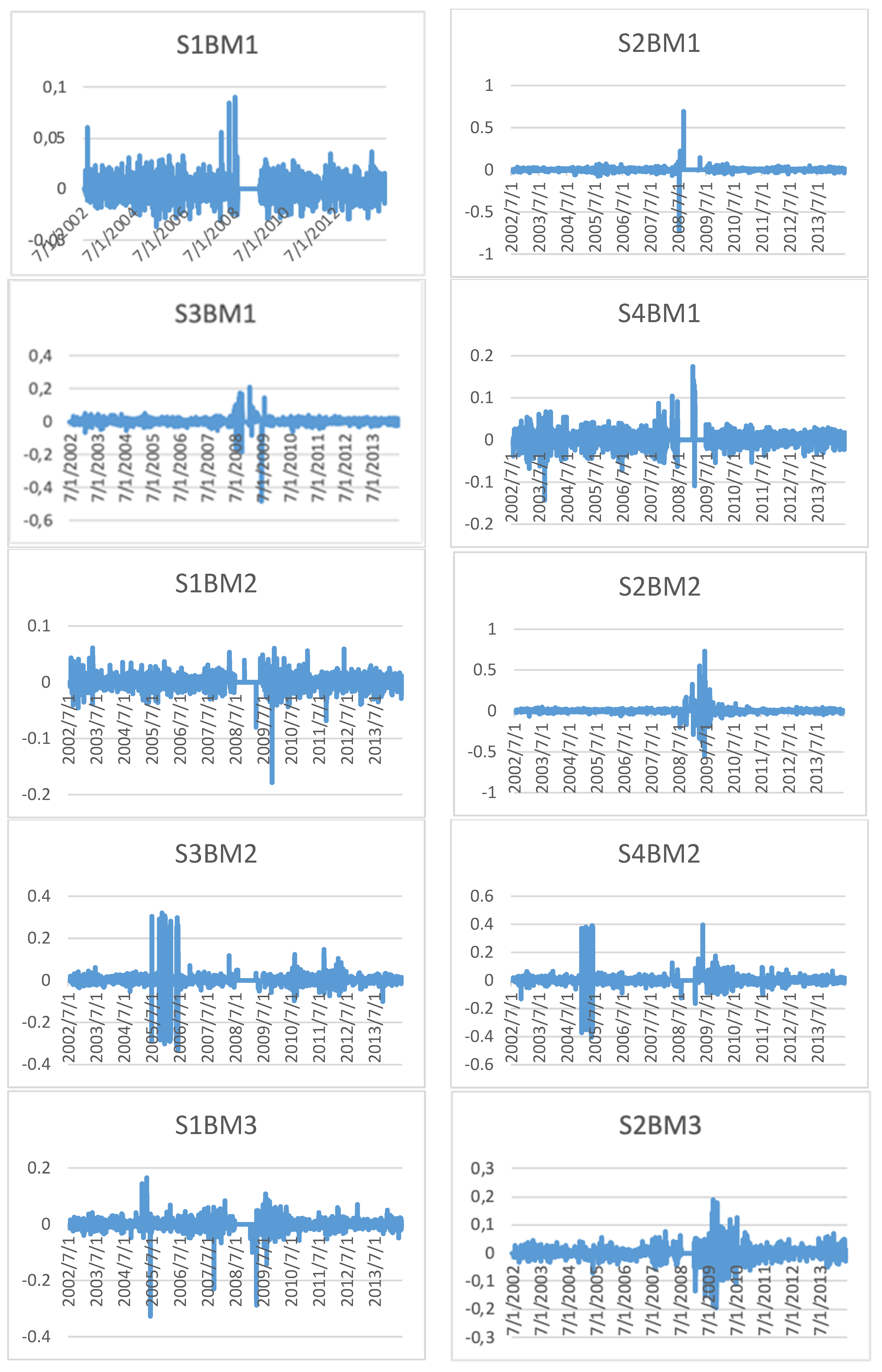
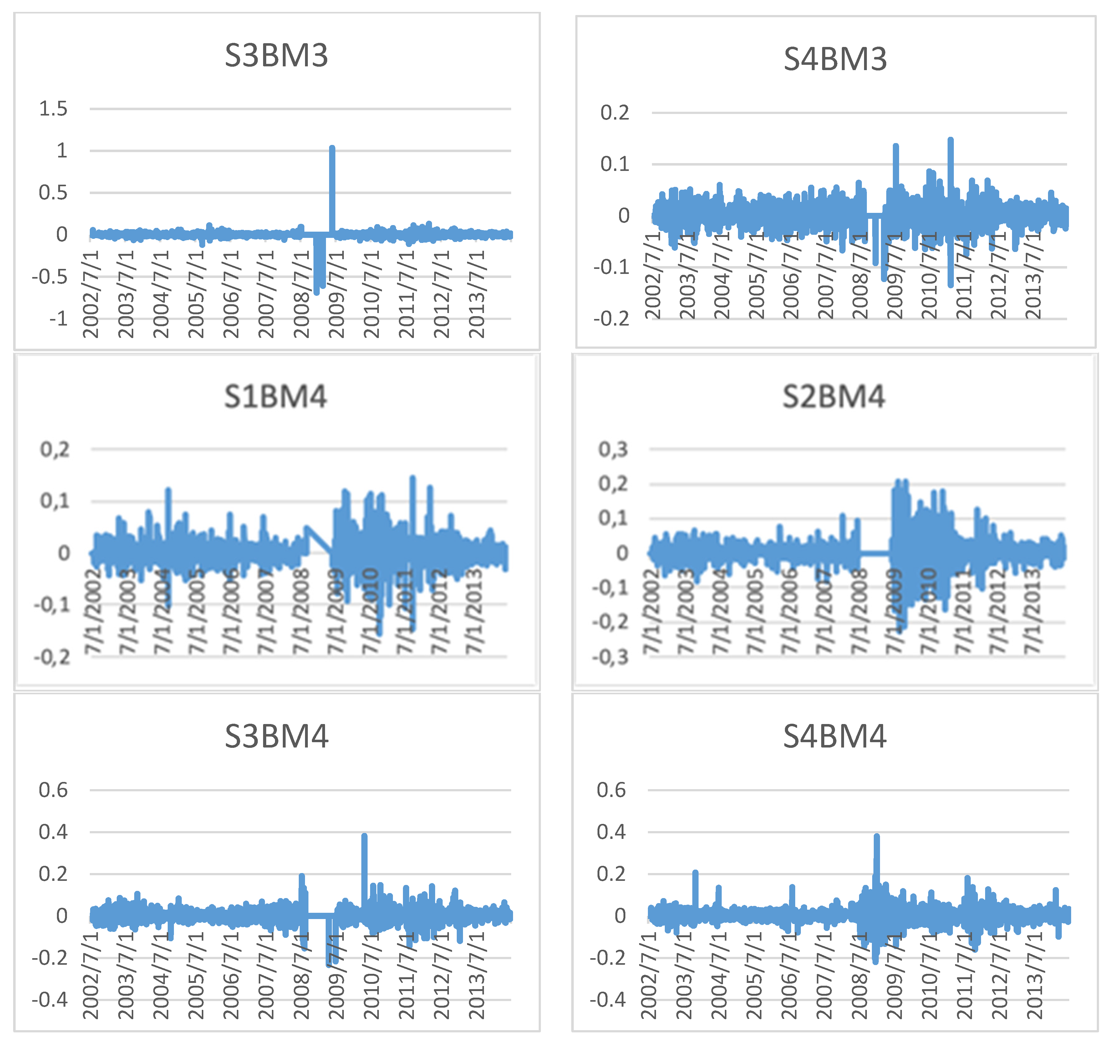
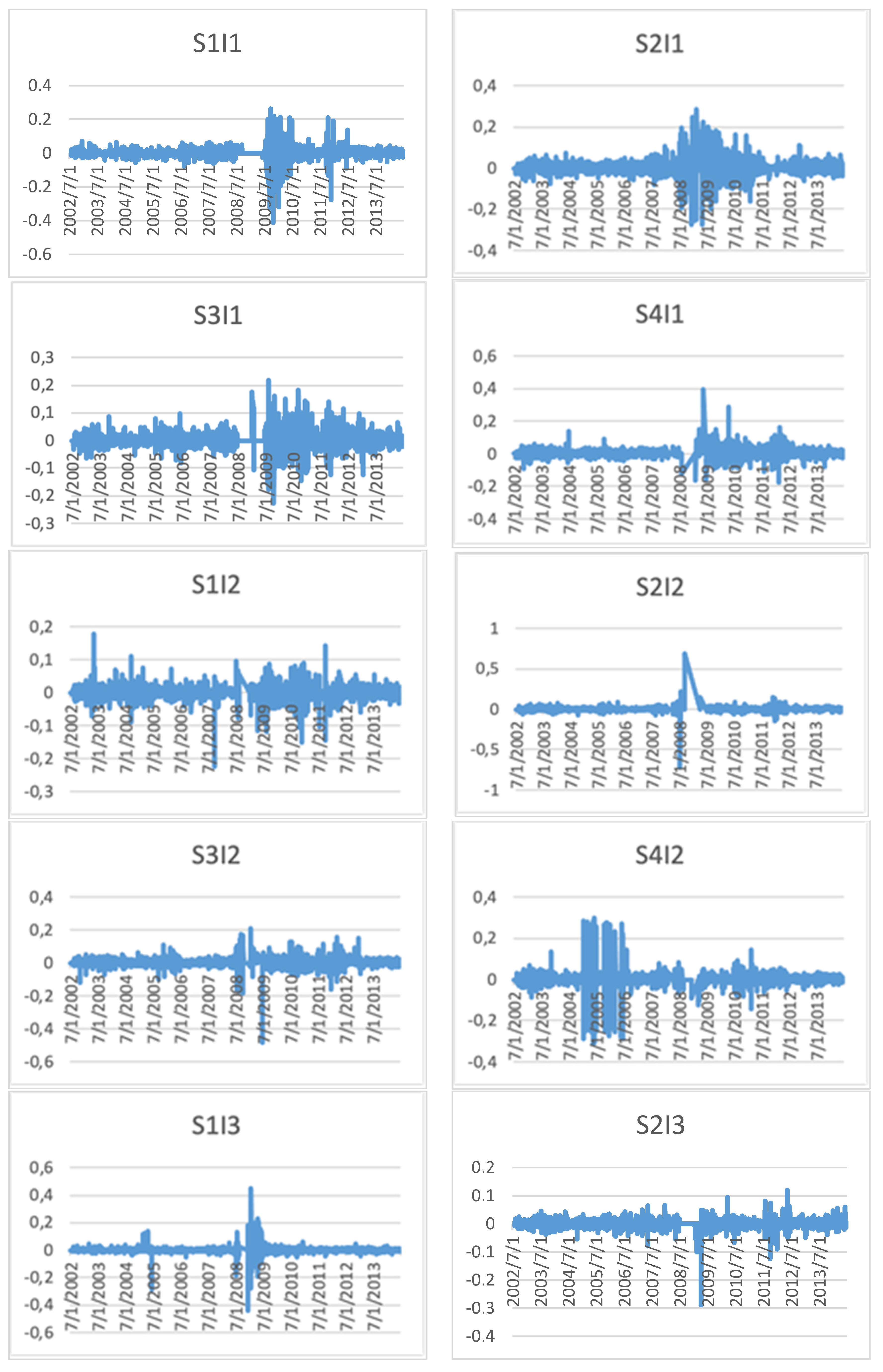
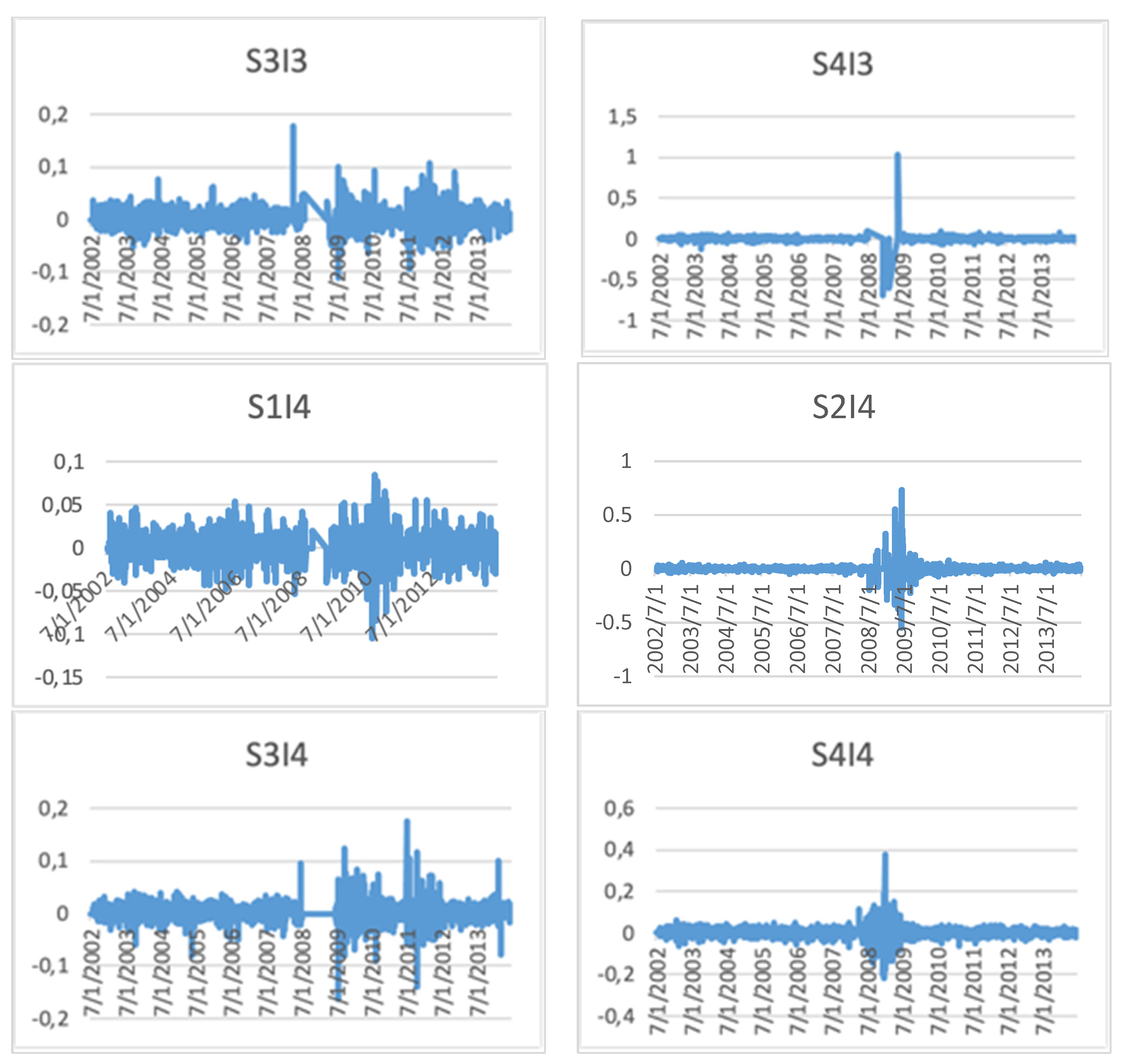
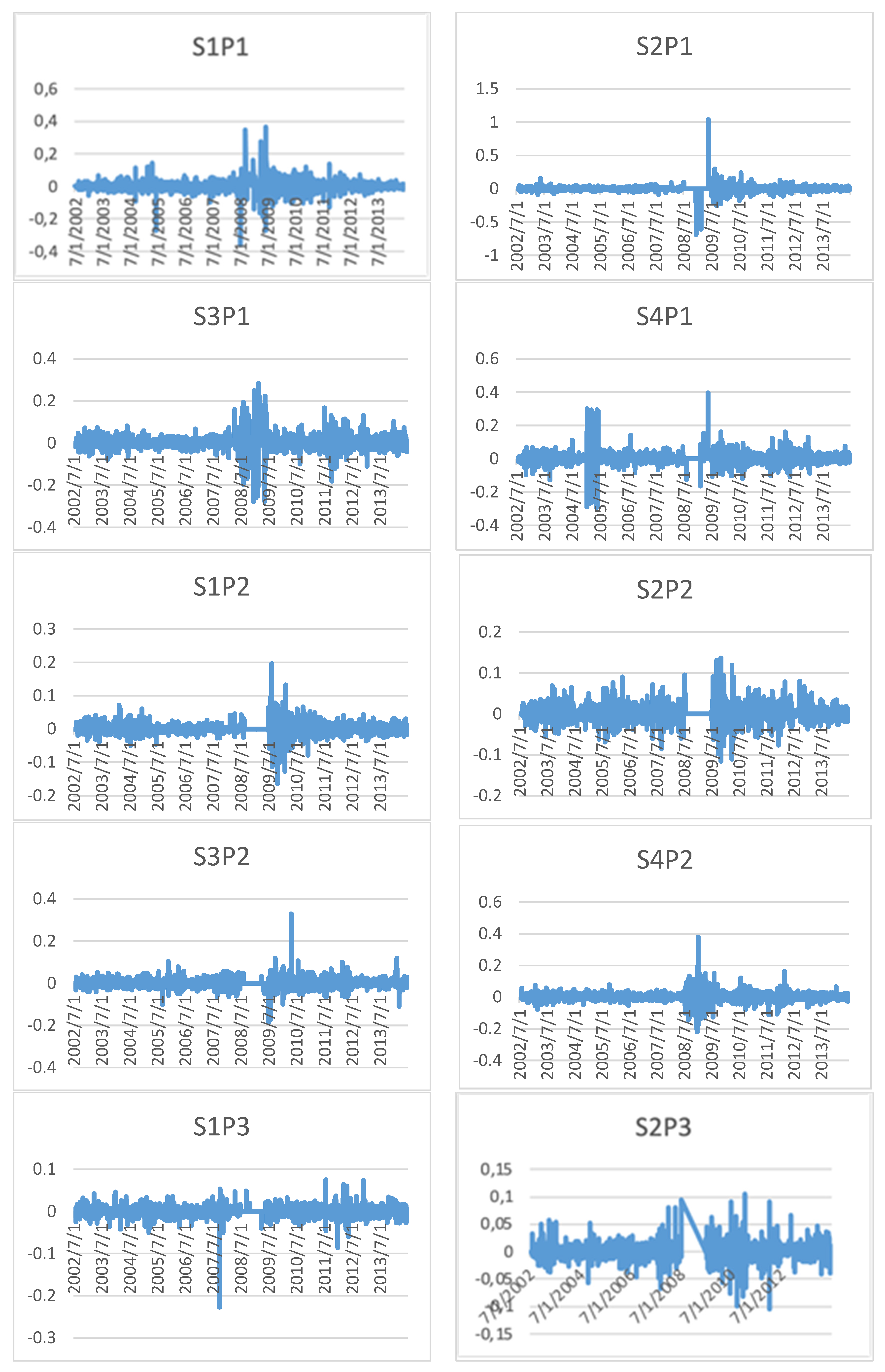
Following are the portfolios based on size, beta, book-to-market ratio, investment, profitability, VaR at 95% and 99% level of confidence, ES or CVaR at 95%, and 99% confidence level. Portfolios have been formed according to the explanatory variables’ size and rest. At first, portfolios have been arranged according to variables other than size factor and quartiles have been made. Under each variable’s quartiles, four quartiles of size have been formed. Average returns of 128 portfolios have been computed from 2002 to 2015 from the data’s stated arrangement. The figures for daily portfolio returns are shown in this study’s Appendix A, Appendix B, Appendix C, Appendix D, Appendix E, Appendix F, Appendix G, Appendix H, Appendix I, Appendix J and Appendix K. The tables represent the significance of whether average returns among portfolios are the same or different.

Table 1. Portfolio average returns based on size and beta. The table represents the average returns of 16 portfolios formed oversize and stock market beta. A total of 527 listed firms are analyzed, from which we dropped firms with negative book-to-market equity from the sample. Firms with missing values and no data were dropped. S1 to S4 represent small to large portfolio stocks, β1 to β4 represents low market beta to high market beta. Diff. (low–high) is the difference of small size with beta portfolios from large size with beta portfolios. p value is the significant value of two-sample t-test of average return difference of two said portfolios. It is tested at 1%, 5%, and 10% levels of significance.

	Size and Beta
	β1	β2	β3	β4
S1	0.08%	0.07%	0.08%	0.12%
S2	0.13%	0.15%	0.16%	0.19%
S3	0.22%	0.19%	0.20%	0.22%
S4	0.27%	0.27%	0.24%	0.21%
Diff. (low–high)	−0.0019	−0.0020	−0.0016	−0.0009
p value	0.0394	0.0000	0.0008	0.2811

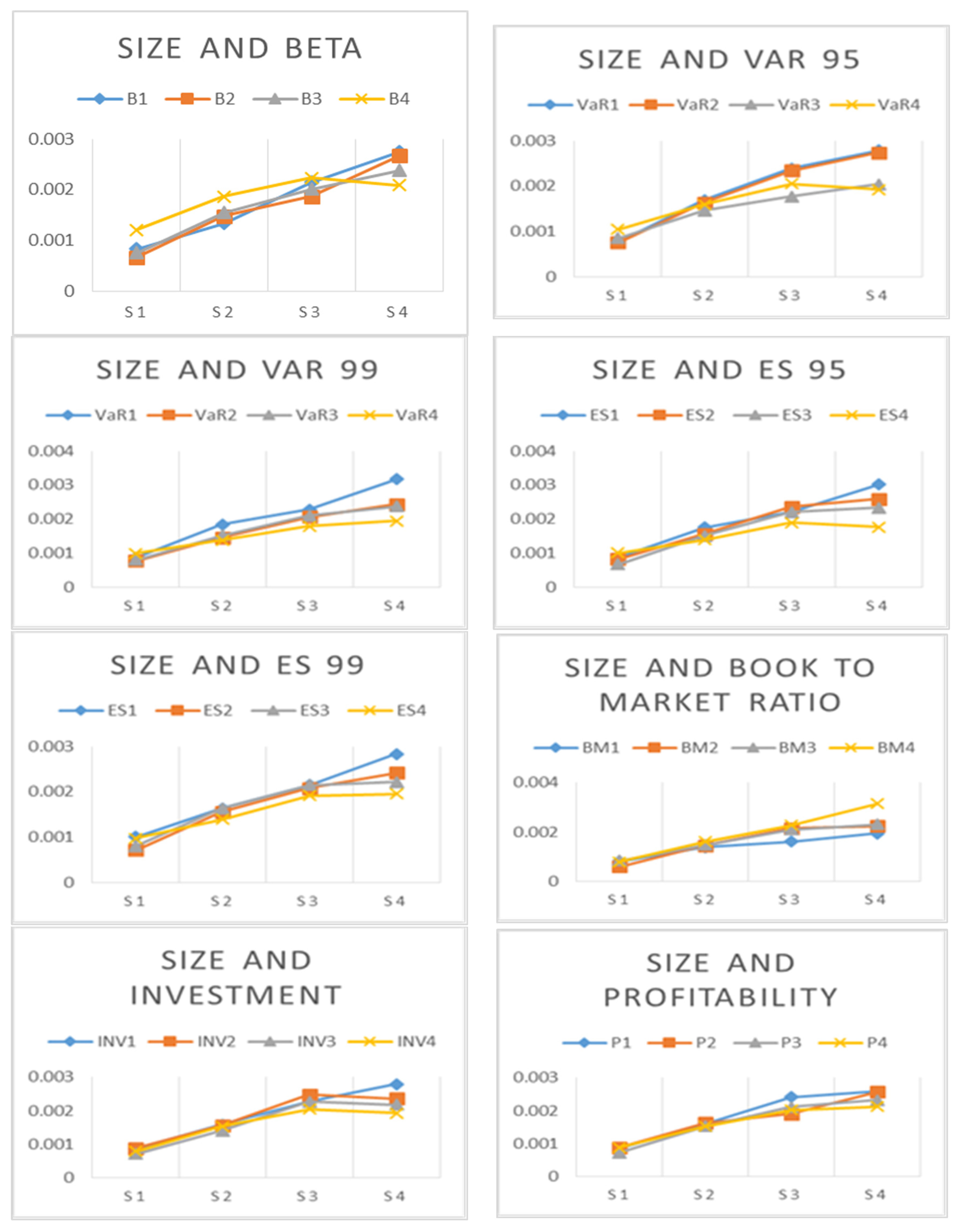
Note: “S” = Size, “β” = beta, p value is significant below 0.10, 0.05, and 0.01.

represents the portfolio’s returns based on size and beta factor. It starts from the small firms “S1” with small beta portfolios” β1” and ends with large firms “S4” with the large beta portfolios “β4”. Portfolios are formed initially by arranging the data according to stocks’ annual market beta value. The study organizes the data according to beta and found three quartiles accordingly. The study has used the yearly market equity data to find the size factor. In each beta quartile, 16 portfolios are formed from four size quartiles. The results suggest that as size increases, return increases, and as market risk (beta) increases the return of securities increases. The average returns of small beta and large beta portfolios change significantly among different size portfolios.

Results indicate that the average return percentage increases from small S1 and low beta β1 to large S4 and low beta β1. The difference between the S1β1 and S4β4 portfolios is −1.9%, significant at a 5% level of significance. The rest of the differences of size with beta portfolios are significant at 1% except for the difference between S1β4, i.e., small size with high beta portfolios, and S4β4, i.e., large size with the high beta portfolio. Overall average returns do not affect the size and beta portfolios. The difference between the small size and low beta (S1β1) portfolios and large size with high beta (S4β4) portfolios is negative 0.12%. The Pakistani manufacturing sector observes the change when portfolios are formed according to size and beta. The results align with Fama et al. [13,18] as average securities increase with size among different beta portfolios. The results have shown Iqbal et al. [28] evidence as nonlinearity among stock returns with portfolios forms with beta across different sizes.

Table 2. Portfolio returns based on size with profitability and investment. The table represents the average returns of 24 portfolios formed oversize and profitability, and 24 portfolios developed oversize and investment. A total of 527 listed firms is analyzed, from which we dropped firms with negative book-to-market equity. Firms with missing values and no data were dropped. S1 to S4 represents small to large portfolio stocks, I1 to I4 represents conservative to aggressive investment stocks, and P1 to P4 represents weak to robust profitability stocks. The difference between small and large portfolios is provided with the p value to measure the significant difference between small and large portfolios.

Panel A. Size and Profitability
	P1	P2	P3	P4
S1	0.09%	0.09%	0.07%	0.09%
S2	0.16%	0.16%	0.15%	0.15%
S3	0.24%	0.19%	0.21%	0.20%
S4	0.26%	0.26%	0.23%	0.21%
Diff. (Small–Large)	−0.00171	−0.00168	−0.00159	−0.00125
p value	0.038	0.0014	0.000	0.074
Panel B. Size and Investment
	I1	I2	I3	I4
S1	0.09%	0.09%	0.07%	0.08%
S2	0.16%	0.16%	0.14%	0.15%
S3	0.23%	0.25%	0.23%	0.20%
S4	0.28%	0.24%	0.22%	0.19%
Diff. (Small–Large)	−0.00193	−0.00148	−0.00146	−0.00114
p value	0.007	0.076	0.041	0.017

Note: “S” = Size, “P” = Profitability, “I” = Investment, p value is significant below 0.10, 0.05, and 0.01.

represents two panels in which the average returns are computed according to portfolios of size with the profitability factor and size with investment factor. These factors are introduced by Fama and French [13] and are widely used in contemporary asset pricing literature. In Panel A, the arrangement of the stocks is according to annual profitability factor. Then, in each quartile of profitability, quartiles according to market equity were found. Daily average returns of each portfolio were accumulated. Lastly, average returns from 2002 to 2015 were found, from small-sized weak profitability portfolios to large-sized robust profitability portfolios. The results show that all profitability-based portfolios’ average returns increase significantly from small-size portfolios to large portfolios. Portfolio average return of size factor does not change significantly among different profitability-based portfolios, which support the findings of Cakici [14]. Small size with profitability factor has lower average returns than large size and profitability portfolios.

Over All average return differences between small size and weak profitability portfolios with large size and robust profitability are –0.13% (The value is calculated by subtracting the portfolio value of S1P1 portfolio from S4P4 portfolio.), significant at 5%. This indicates a high average return of large, robust, profitable PSX firms from average returns of small and weak profitable portfolios.

There is no significant change in the average portfolio return concerning size in the portfolio’s different profitability levels. Panel B of Table 2 represents the stock average returns of portfolios based on size and investment. Firstly, stocks were arranged according to quartiles from conservative (I1) to aggressive (I4) investment portfolios. Four quartiles have been formed of stocks from annual investment data. Under each quartile of stocks, the researcher developed four quartiles according to size. Further average returns have been computed from the small size and conservative investment portfolios S1I1 to large size and aggressive portfolios S4I4, resulting in the construction of average returns of 16 portfolios.

The results show that in each investment portfolio’s average, returns increases with the increase in a firm’s size. There is no significant average return pattern for investment factor in the four quartiles of size portfolios. The returns design does not support Fama et al. [13] findings, but shows some relevance with Kubota et al. [16]. There is a significant difference reported between small stock and large stocks. Large stocks with investment factor portfolios report more average returns than small stocks with investment factor portfolios. Large stocks frequently trade in the market and report stable returns, while small stock trading volumes remain low, making their average returns lower due to price inflexibility.

Results of

Table 3. Portfolio returns based on size and book-to-market ratio. The table represents the average returns of 24 portfolios formed oversize and book-to-market equity. A total of 527 listed firms is analyzed, from which we dropped firms with negative book-to-market equity from the sample. Firms with missing values and no data were dropped. S1 to S5 represents small to large portfolio stocks, B1 to B5 represents small book-to-market to large book-to-market ratio.

Size and BM Ratio
	BM1	BM2	BM3	BM4
S1	0.08%	0.06%	0.08%	0.08%
S2	0.14%	0.14%	0.15%	0.16%
S3	0.16%	0.22%	0.21%	0.23%
S4	0.19%	0.22%	0.23%	0.31%
diff (small–large)	−0.00113	−0.00165	−0.00147	−0.00234
p value	0.000844	0.023175	0.00155	0.000254

Note: “S” = Size, “BM” = Book to Market ratio, p value is significant below 0.10, 0.05, and 0.01.

indicate that the average return percentage increases from small S1 and low BM to large S4 and BM4 portfolios. The well-established cross-sectional analysis provided by Fama and French [18] is tested in the Pakistani stock market, and to some extent, results are different than in developed markets. Growth stock and value stocks report a significant increase in average returns with Pakistan’s market equity. The results of Table 3 are formed firstly by arranging the annual data of PSX according to book-to-market each year. Four quartiles have been developed for each year according to book-to-market ratio. Each year from each quartile, size quartiles are formed. Sixteen portfolios have been constructed each year from the following data.

The average returns of portfolios have been computed annually, and we calculated the time-series average return at the end of the year from 2002 to 2015 for portfolios. S1 represents small stocks, S2 and S3 are the medium-sized stocks, and S4 are the large stocks. BM1 are growth stocks, and BM4 are the value stocks. Portfolios represent the size factor and value factor together. The first difference is between the small stocks with value factor and large stocks with value factor. The result of this difference is significant in Pakistan, as shown by the p values. Overall, S1BM1 and S4BM4 represent the extremes of 16 portfolios. The first represents small stocks with low BM ratio and the latter represents the large stocks with high BM ratio. The overall difference is insignificant in Pakistan.

Table 4. Portfolio returns of size, VaR and ES at 95% level of significance. The table represents the average returns of 24 portfolios formed oversize, and VaR and 24 portfolios created oversize and CVaR at 95% level of significance. A total of 527 listed firms is analyzed, from which we dropped firms with negative book-to-market equity. Firms with missing values and no data were dropped. S1 to S5 represents small to large portfolio stocks, VaR1 to VaR5 represents low VaR to high VaR stocks and CVaR1 to CVaR5 means low to high CVaR stocks.

Panel C: Size and VaR 95
	VaR1	VaR2	VaR3	VaR4
S1	0.077%	0.075%	0.086%	0.105%
S2	0.170%	0.164%	0.146%	0.159%
S3	0.239%	0.234%	0.177%	0.205%
S4	0.278%	0.273%	0.204%	0.193%
Diff. (Small–Large)	−0.0020	−0.0020	−0.0012	−0.0009
p-value	0.0593	0.0000	0.0619	0.0043
Panel D: Size and ES 95
	ES1	ES2	ES3	ES4
S1	0.087%	0.083%	0.068%	0.101%
S2	0.176%	0.156%	0.151%	0.139%
S3	0.220%	0.235%	0.221%	0.190%
S4	0.302%	0.260%	0.233%	0.176%
Diff. (Small–Large)	−0.00215	−0.00177	−0.00165	−0.00076
p-value	0.073866	0.000114	0.0000	0.000266

Note: “S” = Size, “VaR95” = Value at risk at 95% confidence interval, “ES95” = Expected shortfall at 95% confidence interval, p-value is significant below 0.10, 0.05, and 0.01.

highlights two panels of portfolios; Panel C represents the portfolios based on size factor, and equally weighted VaR at 95% level of confidence and Panel D is related to portfolios of size and ES at 95% level of confidence. The first annual value of VaR and ES at 95% has been computed for each stock and is arranged based on the largest to smallest values. Quartiles have been calculated from the organized data. Four quartiles are computed from VaR and ES, and firms are arranged accordingly. According to the quartile of the size factor, each VaR and ES quartile data is contained according to quartile. There are 16 portfolios according to size factor and VaR factor, and there are 16 sizes and ES factor. In panels C and D, it is observed that the average returns from low VaR and ES portfolios do not show any significant pattern. Small-sized and VaR portfolios are significantly different from large and VaR portfolios. Small size and VaR portfolios have lower returns as compared to the large size and VaR portfolios. Looking at the average returns low, VaR has more returns as compared to high VaR stocks. ES stock portfolios follow the same pattern. The overall difference between extreme portfolios, i.e., small size and low VaR portfolios and large size and high portfolio, are insignificant. Similarly, small size and low CVaR or ES portfolios average returns are insignificantly different from large-sized and high CVaR or ES portfolios.

Table 5. Portfolio returns of size, VaR and ES at 99% level of significance. The table represents the average returns of 24 portfolios formed oversize and VaR and 24 portfolios assembled oversize and CVaR. A total of 527 listed firms is analyzed, from which we dropped firms with negative book-to-market equity. Firms with missing values and no data were dropped. S1 to S5 represents small to large portfolio stocks, VaR1 to VaR5 represents low VaR to High VaR stocks and ES1 to ES5 represents low to high expected shortfall stocks.

Panel E: Size and VaR 99
	VAR1	VAR2	VAR3	VAR4
S1	0.086%	0.078%	0.081%	0.099%
S2	0.185%	0.145%	0.152%	0.139%
S3	0.228%	0.206%	0.211%	0.179%
S4	0.317%	0.244%	0.237%	0.194%
Diff. (low–high)	−0.0023	−0.0017	−0.0016	−0.0010
p-value	0.0382	0.0001	0.0129	0.0006
Panel F: Size and ES 99
	ES1	ES2	ES3	ES4
S1	0.101%	0.072%	0.081%	0.098%
S2	0.164%	0.156%	0.163%	0.139%
S3	0.214%	0.208%	0.215%	0.192%
S4	0.283%	0.242%	0.221%	0.196%
Diff. (low–high)	−0.0018	−0.0017	−0.0014	−0.0010
p-value	0.1281	0.0001	0.0000	0.0001

Note: “S” = Size, “VaR99” = Value at Risk at 99% confidence interval, “ES99” = Expected shortfall at 99% confidence interval, p-value is significant below 0.10, 0.05, and 0.01.

represents two panels. Panel E illustrates the portfolios based on size factor and VaR factor at a 99% confidence level. Panel F reports portfolios based on size factor and ES at a 99% confidence level. The results are similar to the previous table except for in Panel E, where the difference between small size with VaR and large size with VaR is insignificant at 1% level of significance. Overall, low VaR has a high return, but it is not valid with VaR to amalgamate with small-sized portfolios. As for size increases, there is a significant increase in returns, but as VaR with size increases, average stock returns decrease. The difference between small size and low VaR and large size and high VaR is negative, which indicates that as size and risk increase the average return also increases.

Panel F provides the ES and size portfolios, and according to the panel high-risk stock with size, portfolios have lower returns than low-risk stock. There is a significant difference between small size and ES portfolios and large size and ES portfolios. Overall, there is a meagre increase in average returns from a small size with low-risk portfolios to large-sized and high-risk portfolios. This finding supports the study’s objective as the VaR and ES measure are the same for all portfolios based on size. The size anomaly, introduced by Benz [26] and Fama and French [17], becomes insignificant when we use VaR- and ES-based portfolios.

3.8. Asset Princing Models

Th main and comprehensive models of time-varying systematic and idiosyncratic risk and returns analysis from equation 11 to 20 are discussed in details in results section. The research aims to analyze and compare the CAPM model presented by Sharpe [8], Lintner [9], and Black [10] with the VaR and ES models. The original CAPM model advocates the single factor, CAPM beta, the effect on returns but with time with the observation of some anomalies with CAPM, certain common risk factors under Arbitrage Pricing Theory (APT) were introduced. The study analyses the impact of the most used factors, namely size and value and recently introduced risk factors, investment and profitability. Inspired by the dividend discount model, Fama et al. [13] specify a different return pattern for conservative investment and aggressive investment and also determine that over time, robust, profitable firms have different returns than weak profitable firms. This section envisages the effect of these factors in time-varying stock excess returns. After a single-factor analysis, this study has compared the traditional three-factor model with the VaR three-factor model and the ES three-factor model. This section checks the significance of market beta with four idiosyncratic factors. In addition to implementing the traditional five-factor model, VaR and ES with idiosyncratic risk factors measure the effectiveness of risk-return trade-off.

4. Results

This section provides analyses of different time-series models. First, the effect of a time-varying single factor is observed with CAPM beta, VaR, and ES. Then, this study analyses the predictability of the traditional three-factor model [18]. The three-factor model’s contribution is analyzed by observing the effect of five systematic risk factors: market beta, VaR at 95% and 99% level of confidence and ES with 95% and 99% level of confidence. The analysis further covers the five-factor model with the market beta, VaR and ES as the controlling systematic risk mechanism. Size, value, investment, and profitability represents the idiosyncratic risk-control mechanism.

Table 6. Single factor systematic risk controlling models. The table represents five models with the dependent variable of excess returns of manufacturing companies (RiRf) listed on the Pakistan Stock Exchange from 2002 to 2014. Independent variables include all systematic risk factors which the study proposed. Excess market returns (Rm-Rf) are calculated from the subtraction of KSE 100 Index returns from the risk-free rate of returns. HLVaR is the subtraction of average returns of High VaR portfolio returns from Low VaR portfolio returns. VaR is observed at both 95% and 99% level of significance. HLCVaR represents subtraction of high ES return stocks from low ES returns stocks. The probability value is provided below, describing the coefficient effect dependent variable’s importance.

Dependent Variable: RiRf
	Model 1	Model 2	Model 3	Model 4	Model 5
RMRF	0.370
	(0.000)
HLVaR 95		0.259
		(0.000)
HLVaR 99			0.125
			(0.000)
HLCVaR 95				0.062
				(0.000)
HLCVaR 99					0.079
					(0.000)
C	−0.001	0.000	−0.001	−0.001	−0.001
	(0.000)	(0.005)	(0.000)	(0.000)	(0.001)
Adj. R Square	0.595	0.442	0.487	0.560	0.501

provides us with the controlling mechanism of systematic risk. The first model represents the traditional SLB CAPM model. The time-varying CAPM model is the most significant single variable model, providing the significant beta value. A one-unit change in market excess returns provides a 0.37-unit stock shift excess returns. VaR and ES betas are proved to be a positive linear function of stock returns. All models offer significant beta values, but VaR at a 95% level of significance provide more effective positive beta value. High minus low VaR at a 99% level of significance report positive risk and return relationship. High-risk CVaR stocks minus low-risk CVaR both provide weak beta values, but the relationship is according to finance theory with positive risk and return connection. VaR and ES models follow EVT to state the extreme values of stocks. High VaR stocks represent a high downside risk, and low VaR stocks represent low downside risk stocks. Both portfolios can be proxy of risk, so high low VaR and ES models portray a firm’s financially distressed position. All models provide a significant positive relationship between risk and returns.

Table 7. Three-factor model using market Beta, VaR, and ES. The table represents five models with the dependent variable of excess returns of manufacturing companies listed in Pakistan Stock Exchange. Independent variables include all the systematic risk factors that the study proposed. Market excess return RmRf calculated from the subtraction of KSE 100 Index returns from the risk-free rate of returns. HLVaR is the subtraction of average returns of High VaR portfolio returns from Low VaR portfolio returns. VaR is observed at both 95% and 99% level of significance. HLCVaR represents subtraction of high ES return stocks from low ES returns stocks. SMB provides a size factor; HML is a value factor. All models give results on the three-factor model with substituting systematic risk factor. Italic probability value is provided below every coefficient value representing the significance of the coefficient effect dependent variable.

Dependent Variable: RIRF
	Model 6	Model 7	Model 8	Model 9	Model 10
RMRF	0.401
	(0.000)
HLVaR 95		0.264
		(0.000)
HLVaR 99			0.118
			(0.000)
HLCVaR 95				0.058
				(0.000)
HLCVaR 99					0.072
					(0.000)
SMB	0.101	−0.035	0.006	0.027	0.025
	(0.000)	(0.001)	(0.582)	(0.018)	(0.032)
HML	0.060	0.030	0.034	0.037	0.041
	(0.000)	(0.001)	(0.001)	(0.000)	(0.000)
C	−0.001	0.000	−0.001	−0.001	−0.001
	(0.000)	(0.000)	(0.000)	(0.000)	(0.000)
Adj. R Square	0.454	0.585	0.491	0.569	0.553

represents the controlling mechanism using market excess returns (RMRF), high minus low VaR at 95% and 99%, high minus low ES or CVaR at 95% and 99% level of significance. Model 6 is the most fitted and significant. Compared with the other models, Fama et al. [18] factor model is the most significant and fitted model. Market beta has a significant positive effect on stock excess returns. Small minus big size factor provides theoretical results. A small size stock has more returns as compared to large size stocks. Value stock has more excess returns as compared to growth stocks.

Model 7 represents a three-factor model with systematic risk measured by VaR at a 95% level of confidence. Model 7 is significant with the significant idiosyncratic risk factor. The size factor follows the finance theory provided by Benz [26], and Fama et al. [17] HML estimates PSX stock returns significantly, as value stocks outperform growth stocks. The intercept of Model 7 is equal to zero, signifying the financial theory that there is no autonomous effect on stock returns besides the independent factors included in the model. The overall model is a good fit and can be used as an alternative to the CAPM model. At 95%, VaR provides us with results similar to the Fama and French three-factor model. VaR at 99% has its significance because it is independent of the size factor’s intermediation. Model 13 reports the positive relationship between risk and return. The HML factor represents firms’ financial distress and has a significant positive effect on stock returns. This finding is in line with Fama and French [29] as they indicated the positive impact of the value factor on stock returns but a negative effect on firms’ earnings.

Time-varying ES or CVaR has a minimal effect on expected stock returns. ES has provided a low but positive explanation of excess stock returns at a 95% and 99% confidence level. At a 1% level of significance, excess stock returns are unresponsive to the size factor. The ES model covers size anomaly. ES three-factor model outperforms Fama et al. [17] three-factor model because the significance of size factor started to reduce from 1% significant level to 5% significant level.

Fama et al. [13] identified the market risk of contemporary unpredictability and segregated the risk into five-factor systematic and idiosyncratic risk factors. The three-factor model’s effect is intact, but the dividend discount model discovers two more factors. One factor that explains the stock market excess return is an investment that we can diversify according to the investor’s investment behavior. The conservative investment strategy will gain low returns, and aggressive investment is risky and volatile, giving high returns or substantial loss. Firm profitability provides the basis of stock returns as we can diversify according to weak and robust profitability. Weakly profitable firms’ stock returns are lower than the robust, profitable firms. According to the five-factor model, a systematic risk factor does not cover the effects of size, value, investment, and profitability. We can diversify our portfolios according to these four idiosyncratic risk factors.

Model 11 of

Table 8. Five-factor model using market Beta, VaR, and ES. The table represents five models with the dependent variable of excess returns of manufacturing companies listed on the Pakistan Stock Exchange. Independent variables include all systematic risk factors which the study proposed. Market excess return RmRf is calculated from the subtraction of KSE 100 Index returns from the risk-free rate of returns. HLVaR subtracts average returns of High VaR portfolio returns from Low VaR portfolio returns. VaR is observed at both 95% and 99% level of significance. HLCVaR represents subtraction of high ES return stocks from low ES returns stocks. SMB provides size factor, HML is a value factor, and RMW estimates the investment factor represented by CMA and profitability. All models offer results of the three-factor model with substituting systematic risk factor. Italic probability value is provided below every coefficient value representing the significance of the coefficient effect dependent variable.

Dependent Variable: RiRf
	Model 11	Model 12	Model 13	Model 14	Model 15
RMRF	0.437
	(0.000)
HLVaR 95		0.280
		(0.000)
HLVaR 99			0.128
			(0.000)
HLCVaR 95				0.059
				(0.000)
HLCVaR 99					0.076
					(0.000)
SMB5	0.152	−0.101	−0.056	−0.020	−0.027
	(0.000)	(0.000)	(0.000)	(0.089)	(0.030)
HML	0.040	0.045	0.043	0.044	0.048
	(0.000)	(0.000)	(0.000)	(0.000)	(0.000)
CMA	0.002	0.012	0.021	0.023	0.022
	(0.824)	(0.117)	(0.012)	(0.007)	(0.008)
RMW	0.002	−0.028	−0.034	−0.027	−0.031
	(0.800)	(0.000)	(0.000)	(0.000)	(0.000)
C	−0.001	0.000	−0.001	−0.001	−0.001
	(0.000)	(0.008)	(0.001)	(0.000)	(0.001)
Adj. R Square	0.480	0.663	0.501	0.473	0.458

represents the traditional Fama et al. [13] five-factor model. RmRf represents the market return minus risk-free rate and proposes a significant positive effect of market risk on stock excess returns. The model suggests the positive, significant relationship of small minus big portfolios to stock returns and high minus low book-to-market portfolios with stock returns, following the theoretical model. According to conservative minus aggressive investment sorted portfolios, the Pakistan stock market cannot be diversifying. It does not affect the stock excess returns, and market beta covered the effect of time-varying investment in Pakistan.

The exciting finding comes into account when applying VaR and ES in the five-factor model. Size effect becomes significantly negative, which means a cross-sectional analysis suggested that big stocks in Pakistan provide more returns than small stocks. Small stocks returns are not volatile due to their low trading volumes on the PSX. Big stocks trading activity is high in the market, and with the economic instability, the stock values of big stocks’ returns are also volatile compared to small stocks. Model 12’ prediction resembles the result of Model 11. Systematic risk factor, VaR, at a 95% level of confidence provides a significant positive relationship with stock excess returns. The size posts significantly negative impact, which is the differing factor between the five-factor and VaR five-factor models. Value factor has a positive significant effect value. VaR 95%, the five-factor model advocates the traditional five-factor model’s findings by predicting the insignificant effect of CMA on stock excess returns.

In Model 12, robust, profitable firms provide less and stable returns than weak profitable firms, whose returns are more volatile. Model 13 uses VaR 99% as a systematic risk factor and findings are on track with Model 12. Stock excess returns sensitivity reduced with VaR 99 beta, size, value and RMW factor due to CMA minor positive significant effect on stock excess returns. The size factor is negatively significant; value factor explains stock returns positively. ES five-factor models provide weak results. It is similar to VaR models as it offers the considerable positive effect of systematic risk. All idiosyncratic risk factors are significant in Model 14. Small-size stocks negatively explain stocks, and large-sized stocks present excess stock returns positively. CMA estimation of excess stock returns is positive and highly significant. Robust, profitable firms hurt stock excess returns as compared to weak profitable firms. Model 15 is concerned with the five-factor model with the inclusion of ES at a 99% level of confidence. The beta of CVaR 99 significantly affects stock returns advocating the Markowitz [30] model of positive risk and return analysis. Idiosyncratic risk factors prediction is under Model 14. The sensitivity of stock excess returns and idiosyncratic risk factors increases with the increase in the level of confidence of ES, which advocates the proposition of Degiannakis et al. [31].

Their study indicated that VaR and ES lost its effectiveness when confidence was increased to 99%. At CVaR 99, size factor negatively affects the stock returns, and it is significant at a 5% level of significance. The size factor of Model 14 is significantly negative at a 10% level of significance. CMA provides substantial positive effect, and RMW influences stock returns significantly but in the opposite direction.

Table 9. Six-factor model. The table represents four models with the dependent variable of excess returns of manufacturing companies listed on the Pakistan Stock Exchange. Independent variables include all systematic risk factors which the study proposed. Market excess return RmRf calculated from the subtraction of KSE 100 Index returns from a risk-free rate of returns. VaR is considered another risk factor with the systematic risk factor in this table. HLVaR subtracts average returns of High VaR portfolio returns from Low VaR portfolio returns. VaR is observed at both 95% and 99% level of significance. HLCVaR represents subtraction of high ES return stocks from low ES returns stocks. SMB provides size factor, HML is a value factor, RMV estimates investment factor represented by CMA and profitability factor. All models give results on the six-factor model. Italic probability value is provided below every coefficient value representing the significance of the coefficient effect dependent variable.

Dependent Variable: RiRf
	Model 16	Model 17	Model 18	Model 19
HLVaR95	0.183
	(0.000)
HLVaR 99		0.085
		(0.000)
HLCVaR 95			0.034
			(0.000)
HLCVaR 99				0.049
				(0.000)
RMRF	0.355	0.414	0.421	0.427
	(0.000)	(0.000)	(0.000)	(0.000)
SMB5	0.056	0.105	0.133	0.130
	(0.000)	(0.000)	(0.000)	(0.000)
HML	0.038	0.035	0.036	0.038
	(0.000)	(0.000)	(0.000)	(0.000)
CMA	−0.004	−0.002	−0.001	−0.001
	(0.520)	(0.782)	(0.932)	(0.834)
RMV	−0.005	−0.005	0.000	−0.002
	(0.380)	(0.378)	(0.941)	(0.695)
C	0.000	0.000	−0.001	−0.001
	(0.001)	(0.000)	(0.000)	(0.000)
Adj. R Square	0.553	0.609	0.499	0.667

provides four contributory models, representing six factors. Fama and French (2014) provided the body of knowledge with five factors. VaR represents the worst expected loss of stock or portfolio of stocks at a certain confidence level with some time horizon (Jorion, 2002, 2006). It means the worst expected loss of securities and, unlike market beta, it measures only downside returns of securities. The study adds VaR and ES into the model to estimate its idiosyncratic effect on stock returns. Model 16 of Table 9 provides information regarding the six-factor model, using excess stock return RiRf as the dependent variable, and independent variables are market excess returns (RMRF), VaR at 95% level of confidence, small minus large stocks (SML), high value minus low-value stocks (HML), conservative minus aggressive investment stock (CMA) and robust minus weak profitability stocks (RMW).

This model’s fitness is higher than all the time-series models, and the model is significant. VaR is considered highly positive and significant among idiosyncratic risk factors. Stock excess return is more responsive to the VaR 95 factor than the rest of the factors. Market beta represents the systematic effect on stock returns and stock returns are highly responsive towards market beta, which indicates the significance of systematic risk and returns trade-off. The model specifies the positive effect of size and value factors and its prediction. RMW and CMA provide an insignificant impact on stock returns.

Model 16 suggests the four-factor model in which market beta, VaR, size and value are included. Model 17 uses VaR at a 99% level of confidence, and results show that market beta strength increases to predict stock returns as we reduce VaR’s significance level. This finding indicates the alternation of market beta with VaR, as VaR significance reduces in the model size factor effect on excess stock returns, which is also increasing, and means that VaR captures the impact of the size factor. The HML factor is significant in the Pakistani stock market. Model 17 also indicates the insignificant results of RMW and CMA.

Model 18 uses CVaR 95 with Fama et al. [13] five-factor model and indicates that CVaR 95 has a minimal positive but significant effect on excess stock returns. The market beta slope is getting stronger as VaR’s effect is getting weaker, which indicates that the effect of VaR enhances the impact of beta reduces, and implications of other idiosyncratic factors such as size also reduce. VaR is an alternative to market beta. This evidence gets stronger when we analyze Model 18, which shows a similar result reported in Model 19. No distinction is written according to firms’ profitability; whether firms are weak profitable or robust profitable, the systematic risk covers the factor’s effect. The same is whether there are conservative investment firms and aggressive investment firms; no diversification is required because systematic market risk addresses evidence of such danger to investors. Both VaR and ES post significant positive effect on stock returns. This finding shows strong evidence regarding risk-return trade-off. VaR and ES’s inclusion reduced the model’s misspecification bias, supporting Degiannakis et al. [31] findings. As Dimitrakopoulos et al. [32] discussed, the enhanced predictability of VaR, their study’s results show the consistent linearity related to VaR and ES towards stock returns strongly support the predictability of the risk factors.

5. Discussion and Conclusion

5.1. One-Factor Model

The market excess return has the highest coefficient value in predicting the stock excess returns. The findings are in line with the Sharpe [8], Lintner [9] and Black [10]. It is according to the assumption of risk aversion. International literature reports the positive effect of market beta on stock excess returns. This is in line with Fama et al. [23], Trimech et al. [33] and Kubota et al. [16]. VaR at 95% and 99% confidence levels produces significant positive results. At 95% and 99%, ES has the lowest effect on stock excess returns. However, the factor has a significant positive coefficient, which supports the assumption of risk aversion. Gong et al. [34] reported positive VaR and ES, which tests their effect on stock excess returns. This section’s findings support Degiannakis et al. [31] results, who state that VaR and ES at a 95% level of confidence have better explanatory power than VaR and ES a 99% level of confidence. Further, it meets the hypothesis because all systematic risk factors significantly affect stock returns. The findings also complete the study’s objective because VaR and ES can be used as the mimicking factors to CAPM.

5.2. Three-Factor Model

According to Fama et al. [17], the traditional three-factor model supports all the findings proposed by this study. VaR and ES are positively related to stock returns, but the effect reduces as confidence increases. The size factor has a significant positive impact on CAPM and the multifactor model supporting Abhakorn et al. (2013) findings. The size factor becomes negative when VaR at a 95% level of confidence is used as the systematic risk factor. Size becomes insignificant with VaR, as the systematic risk factor is at a 99% level of confidence. HML has a significant positive effect on stock returns with all three-factor models. Abhakorn, Smith, and Wickens [35] reported that the value factor adds to the study’s explanation. According to whom value has a negative impact on stock returns, the value effect rejects Gong and Weng [34] results.

5.3. Five-Factor Model

All the systematic risk factors have a positive significant coefficient to predict stock excess returns’ time-series. The CAPM beta has a greater significance as compared to other systematic risk factors. SMB remains positive with the traditional five-factor model proposed by Fama and French [13], but it becomes negative when VaR and ES are used to control systematic risk.

HML in all the models remains significant and positive, supporting the result reported by Drew et al. [36] and Trimech et al. [33]. Abhakorn et al. [35] indicate HML as a factor that adds to the model’s explanation. The study goes another way in response to declaring HML as the redundant factor with the inclusion of investment and profitability factor [13].

Kubota and Takehara [16] findings are relevant to the Pakistan stock market. They indicated that the Fama et al. [19] five-factor model has no significance in the Japanese market. The current study results support this finding while applying the Fama et al. [22] five-factor model. Both profitability and investment factors failed to explain the five-factor model’s stock excess returns.

5.4. Six-Factor Model

This study introduces a six-factor model by including the VaR and ES at 95% and 99% confidence levels to the Fama et al. [18] five-factor model. The result shows the positive effect of CAPM beta with all the VaR and ES risk factors. However, the magnitude of CAPM beta reduces with VaR and ES’s inclusion. SMB and HML have a positive and significant effect on stock excess returns. CMA and RMV remain insignificant, as reported by the five-factor model in this study.

5.5. Main Findings

The study comprises the models representing the time-series analysis of risk and returns trade-off. The Pakistani stock market supports the traditional CAPM model by analyzing the one-, three-, and five-factor models. Excess market returns significantly and positively envisage the stock excess returns in the one-, three-, and five-factor models. According to the Fama et al. [17] theory implications for the Pakistani stock market, the traditional time-varying three-factor model also provides significant results. The five-factor model in time-series setup has failed to be implemented in the Pakistani stock market. The results are supported by Kubota et al. [16] in the Japanese market, where the five-factor model failed to be applied. The study’s objective is met because the coefficient of CAPM, VaR, and ES are positive and significant in explaining the stock returns. SMB and HML factors meet the study’s hypothesis by significantly affecting the stock returns. Investment and profitability factors are proved to be redundant in Pakistan’s emerging market. So, the null hypothesis is accepted for the investment and profitability factor. The study proposes the substantial implications for future research for the six-factor model application as there is a significant idiosyncratic tail dependence proposed by the sixth factor (VaR and ES).

5.6. Research Implications

This study’s empirical investigation helps to understand the complexity of asset pricing models in emerging economies at the micro and macroeconomic level. Furthermore, investors, policymakers and regulators can address the following issues:

• The risk-return trade-off complexity
• Optimized asset pricing models
• Negativity bias in the market
• Risk-averse behavior of investors in emerging markets
• The predictable model capacity of outliers

The proposed model’s practicability is easy to implement in emerging economies like Pakistan.