Abstract
The system designed to accomplish the engraving process of a rotating band projectile is called the gun engraving system. To obtain higher performance, the optimal design of the size parameters of the gun engraving system was carried out. First, a fluid–solid coupling computational model of the gun engraving system was built and validated by the gun launch experiment. Subsequently, three mathematic variable values, like performance evaluation indexes, were obtained. Second, a sensitivity analysis was performed, and four high-influence size parameters were selected as design variables. Finally, an optimization model based on the affine arithmetic was set up and solved, and then the optimized intervals of performance evaluation indexes were obtained. After the optimal design, the percent decrease of the maximum engraving resistance force ranged from 6.34% to 18.24%; the percent decrease of the maximum propellant gas temperature ranged from 1.91% to 7.45%; the percent increase of minimum pressure wave of the propellant gas ranged from 0.12% to 0.36%.
1. Introduction
The gun launch process can be simply introduced as follows: first, the propellant particles burn and produce propellant gas, and then the propellant gas pushes projectile base to move along translation–rotation trajectory to the projectile leaves the muzzle. The gun launch process can be divided into three steps, namely the propellant combustion, the engraving process of the projectile rotating band and the high-speed movement of the projectile. As for the engraving process of the projectile rotating band (engraving process for short in this paper), it has two main functions. One is making the projectile rotate and improving the movement stability of the projectile in the air, and the other one is avoiding the spillage of the propellant gas.
The system, which is designed to accomplish the engraving process of the rotating band, is called a gun engraving system, and it consists of two parts, namely the propellant part and the mechanical part. Many researchers have studied the gun engraving system model and engraving process in relation to the research of the mechanical part of the gun engraving system. Various types of rotating bands were manufactured by Wu et al. [1,2,3,4,5], and the gas gun was used to conduct a series of contrast tests. He investigated the influence factors of the engraving process, which include load type, shape and dimension of the rotating band. By proposing the dynamics calculation model, Sudarsan et al. [6] studied the short start pressure of the engraving process on different calibers of the gun and discussed the dependent parameters. Sun et al. [7] established the three-dimensional finite element model of the gun engraving system and simulated the dynamic response of the rotating band on different charges. In relation to the research of the gun propellant combustion and load calculation. Measuring the propellant combustion law by closed bomb vessel, Monreal-González et al. [8,9] proposed an interior ballistics model of two-phase flow and the calculated pressure data matched well with the experimental firing data. The two-phase flow model, which is described propellant combustion characteristics, was built by Otón-Martínez et al. [10], and the relative variable values obtained by his model were consistent with the data obtained by IBHVG2 software and experiment. MacCormack-TVD and Rusanov numerical schemes were employed by López et al. [11] to solve the propellant detonation model, and the contrastive results showed that MacCormack-TVD is suitable for solving this kind of detonation problem. Although many researchers have studied either the mechanical or the propellant part of gun engraving systems, respectively, the separate models cannot describe the interactive characteristic of each part. In this paper, the fluid–solid coupling model of the gun engraving system, which consists of both mechanical part and propellant part, is established.
The size parameter of an object is an important influence factor on its performance. Moreover, the relationship between the size parameter of the object and its performance is widely studied in the traditional design fields such as welding engineering [12] and newly developing design fields such as biomechanical engineering [13]. Likewise, the size parameters of the gun engraving systems also play an important role in its performance. Furthermore, there exists uncertainty due to manufacturing errors in the gun engraving systems. The values of these uncertainties may be tiny, but their coupling effect will produce a critical impact on the gun engraving system. Thereby, considering the parameter uncertainties, it is necessary to carry out the size parameter optimization of the gun engraving system for higher engraving process performance. Although there is little research in this area, there are many efforts in other fields. At present, there are mainly random programming methods, fuzzy programming methods and interval optimization methods in the field of uncertainty optimization problems [14]. In interval optimization, the uncertain parameters are described by interval numbers. Only the upper and lower bounds of the parameters need to be known; the precise probability distribution or the fuzzy membership function is unnecessary. Therefore, the interval optimization method is employed in this article. The traditional interval optimization method [15,16] is a two-layer nested method, which is very time-consuming due to the inner layer optimization. Transforming the two-layer nested optimization into a single-layer one is an efficient solution to avoid inner layer optimization. Jiang et al. [15] transformed the nonlinear objective function and constraints into an approximate linear model through first-order Taylor series expansion using the sequential linear programming method. The intervals of the objective function and constraints were obtained; thus, the problem was transformed into a single-layer deterministic problem. Chen et al. [17] studied the uncertain optimization problem of a multi-degree-of-freedom vibration system. By combining interval extension and first-order Taylor expansion, the boundary of nonlinear function under variable disturbance was approximately solved so as to convert the problem into a single-layer optimization problem. However, using first-order Taylor expansion to transfer nonlinear problems into linear problems will bring errors that cannot be ignored. Hence, Liu and Yan [18] proposed an improved Taylor expansion based method considering monotonicity. Zhou and Li [19] proposed the concept of Utopian Point based on the sequential quadratic programming method. The upper and lower bounds of the corresponding inner optimization can be obtained only by performing matrix operations, thus transform the problem into a single-layer deterministic problem. Wu et al. [20] proposed an interval uncertainty optimization method combining the Chebyshev surrogate model and higher-order Taylor expansion. It could effectively inhibit the interval expansion problem caused by interval arithmetic and could directly calculate the upper and lower bounds of interval functions. Wang et al. [21,22] introduced the feedforward neural networks to compute the derivative information in Taylor expansion, thus proposed a novel interval optimization algorithm. However, the calculation of the abovementioned optimization methods is toughly complicated. In this paper, a nonlinear uncertainty optimization method based on an affine algorithm is introduced. By using affine arithmetic to calculate the uncertain objective function and constraint, its interval bounds can be calculated directly so that the two-layer nested uncertain optimization can be transformed to a single-layer uncertain optimization problem.
Multiobjective optimal design can improve the whole system performance significantly [23,24,25,26], and the optimal design of the gun engraving system also belongs to the category of multiobjective optimal design. On the other hand, high-efficiency [27,28] and low-cost [29] are also pursued by designers in the field of optimal design. The former optimal design of the gun engraving system needs a series of launch experiments, and therefore it costs much budget and time. For obtaining higher performance, this paper will provide an optimal design scheme of the gun engraving system, and its process is exhibited in Figure 1. This paper is organized as follows: In Section 2, the fluid–solid coupling computational model of the gun engraving system is set up, and the dynamic response of the engraving process is analyzed. Then the twelve related size parameters are selected for sensitivity analysis in Section 3. In Section 3, the sensitivity analysis on the engraving resistance force , temperature T and the pressure wave of the propellant gas are performed. Then four high-influence size parameters are selected as design variables for optimization in Section 5. In Section 4, the affine arithmetic-based method is validated by the numerical example and is adopted for optimization in Section 5. In Section 5, the optimization of the gun engraving system is carried out, and then the optimized intervals of performance evaluation indexes are obtained. In addition, this paper has two main novelty contents. One is that building a fluid–solid coupling computational model of the gun engraving system, which can take the fluid–solid interaction into account and analyze the comprehensive performance. The other one is that the affine arithmetic-based method is adopted for optimization, which has high accuracy and high computational efficiency.

Figure 1.
Flow chart of the present work in this paper.
2. Modeling of the Gun Engraving System and Experimental Investigation of Engraving Process
2.1. Introduction of Engraving Process
On the structural design of a gun, usually, there are one or two rotating bands encircling the projectile and dozens of spiral riflings attaching at the bore surface, as exhibited in Figure 2. For most types of rotating bands, their materials are copper alloy because the strength of the copper alloy is lower than that of steel, which is adopted by the gun barrel and riflings.
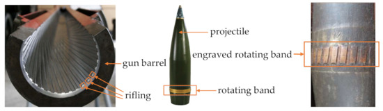
Figure 2.
Exhibition of physical pictures of the gun engraving system.
Figure 3 represents the size comparison among the first rotating band diameter Dr, the second rotating band diameter Dl and barrel bore diameter Db. As can be seen, the value of Dl (167 mm) is higher than the value of Dr (164 mm). This design purpose is to generate a contact surface between the second rotating band and forcing cone before the projectile moves, which can ensure the location of the projectile.

Figure 3.
Exhibition of the size comparison between D r, Dl and Db.
In addition, the values of Dr (164 mm) and Dl (167 mm) is higher than the value of Db (160 mm). Due to the size relationship, there exists a contact surface among these two rotating bands, the riflings and the bore surface after the projectile moves.
Figure 4 represents the schematic diagram of the gun engraving system, which has the section of the gun barrel, and here we amplify and straighten one spiral rifling for better display. This spiral rifling can be divided into two segments, namely the initial segment and the formal segment. The rifling height at the initial segment gradually increases for the sake of getting a smooth and stable engraving process.
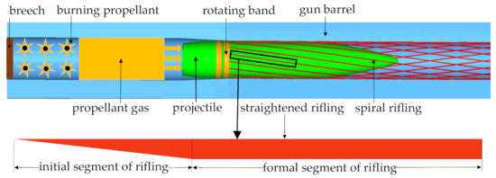
Figure 4.
Schematic diagram of the engraving process and exhibition of straightened rifling.
The engraving process can be described as follows: First, the projectile is pushed by the propellant gas. Subsequently, the contact occurs between the rotating band, riflings and bore surface. Thus, the projectile starts to translate and rotate. When the rotating band moves across the initial segment of riflings, the engraving process finishes, and at this time point, the velocity of the projectile is called engraving-completion velocity. After the engraving process, the rotating band is engraved, as exhibited in Figure 2.
2.2. Investigation of Engraving Process by Real Gun Launch Experiment
To investigate the engraving process, previous experiments have utilized simplified instruments. In this paper, considering the validation of the model of the gun engraving system, a real gun launch experiment was carried out. In Figure 5, the schematic diagram of the experiment is exhibited in the center with a black dotted line, and the red arrows point to the corresponding physical pictures.

Figure 5.
Schematic diagram and the physical picture of real gun launch experiment.
The launch experiment is described below. A hole was dug throughout the gun barrel, and the pressure sensor was fixed in this hole to measure the propellant gas pressure at the projectile base. The measured data were saved in a data processing computer, as shown in Figure 6a. Furthermore, the projectile velocity was also obtained. More specifically, we connected the projectile rigidly with a calibrated bar, which can move with the projectile. A high-speed camera was used to collect the movement data of the calibrated bar. Moreover, the velocity of the calibrated bar is equal to that of the projectile. Finally, the projectile velocity is shown in Figure 6b.
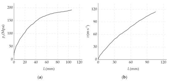
Figure 6.
(a) Pressure at the projectile base vs. projectile displacement; (b) projectile velocity vs. projectile displacement.
2.3. Modeling of the Gun Engraving System and Results of Dynamic Response
As mentioned above, the gun engraving system contains the propellant part and the mechanical part. Correspondingly, the fluid–solid coupling model of the gun engraving system contains two submodels, namely the launch-load model (the fluid submodel) and the finite element model (the solid submodel).
2.3.1. Launch-Load Model and its Calculation Results
The force exerted on the projectile base comes from the propellant gas, and the interior ballistics model is used to describe the propellant combustion law and obtain the state value of the propellant gas [30], especially the pressure data. Based on multiphase flow theory [31], we have made minor modifications in the original launch-load model, which can be found in reference [30]. The minor modified launch-load model has five main equations, as expressed below.
The mass conservation equation of the propellant gas:
The momentum conservation equation of the propellant gas:
The energy conservation equation of the propellant gas:
The mass conservation equation of solid-phase propellant:
The momentum conservation equation of solid-phase propellant:
The symbol meanings in the above equations are listed in Table 1. In addition, MacCormack [32] difference scheme is used for solving the equations, and it has second-order accuracy, as expressed in Equation (6).

Table 1.
The symbol meanings in the model of the launch load.
After the calculation, the three-dimensional displacement–time–temperature data of the propellant gas and the two-dimensional time–temperature data of the propellant gas at the point where x = 0.9 m are shown in Figure 7a,b, respectively. Here the displacement represents the distance from the propellant gas to the gun breech, and it will increase after the projectile moves. Hence, Figure 7a,b contains the blank space at each right side, and the curves represent the trajectory of the projectile.
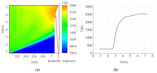
Figure 7.
(a) Displacement–time–temperature data of the propellant gas; (b) time–temperature data of the propellant gas at 0.9 m.
The high-temperature of the propellant gas causes the erosion phenomenon on the internal surface of the gun barrel, and the erosion degree affects the service life of the gun barrel. Hence the temperature value of the propellant gas T is the first performance evaluation index during the engraving process. In this paper, there are totally three performance evaluation indexes, and they are described in Figure 8.
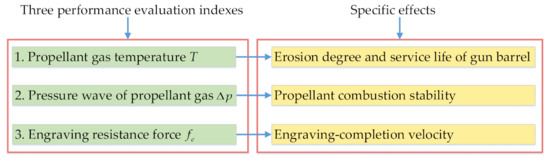
Figure 8.
Three performance evaluation indexes and their corresponding physical effects.
The three-dimensional displacement–time–pressure data of the propellant gas and the two-dimensional time versus pressure wave data of the propellant gas are shown in Figure 9a,b, respectively. The pressure wave is calculated by the way that pressure at breech minus that at the projectile base, and the minimum value of pressure wave represents the propellant safety. The higher the minimum value of the pressure wave is, the better the combustion stability of the propellant is. Hence, the value of pressure wave is the second performance evaluation index, which is used to evaluate the combustion safety during the engraving process.

Figure 9.
(a) Displacement–time–pressure data of the propellant gas; (b) time–pressure wave data of the propellant gas.
The displacement–pressure data at the projectile base, which are extracted from Figure 9a, are shown in Figure 10. As can be seen, the calculation data match well with the experimental data from Figure 6a. Hence, the accuracy of the launch-load model is validated.
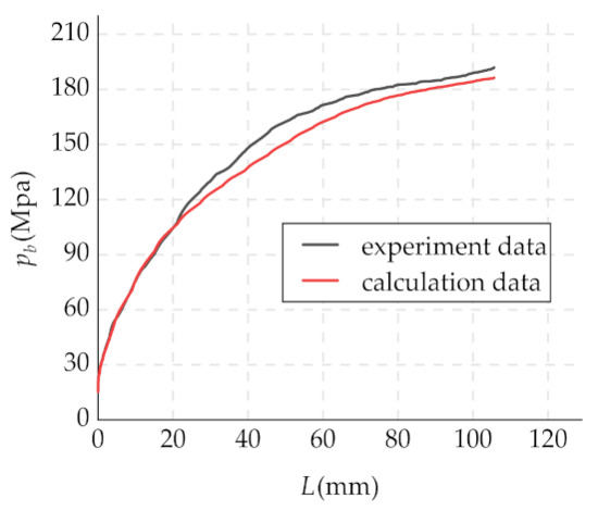
Figure 10.
Comparison of displacement–pressure data of the projectile by calculation and experiment.
2.3.2. Finite Element Model and its Simulation Results
The finite element model of the mechanical part of the gun engraving system is built by Hypermesh software, as shown in Figure 11. Here, the cross-section of the rotating bands is enlarged for better display, as shown in Figure 12. Specifically, this model contains four components, namely the gun barrel, the rifling, the projectile and the rotating band. In the model, there are 48 riflings and 2 rotating bands in total. In addition, the whole finite element model has 1,443,203 elements and 1,285,561 nodes, and all element types are hexahedron for computational accuracy. Peculiarly, considering the large deformation of the rotating bands, the element sides of the rotating bands range from 0.3 mm to 0.5 mm, while the element sides of other components are from 3 mm to 6 mm. The propellant gas pressure, which is calculated by the launch-load model in Section 2.3.1, is applied on the projectile base by Vuamp subroutine in Abaqus software. The Vuamp function offers a data exchange interface between the launch-load model and the finite element model. Hence, the integrated gun engraving system model is a two-way fluid–solid coupling model, and there is an interaction between the launch-load model and the finite element model. Finally, the dynamic response data of the rotating band and projectile are calculated by Abaqus explicit solver.
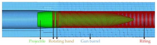
Figure 11.
Three-dimensional finite element model of the gun engraving system.
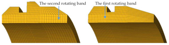
Figure 12.
Cross-section of finite element model of the rotating bands.
The basic material parameters are listed in Table 2. Considering the large deformation of rotating bands, the Johnson–Cook material constitutive model and Johnson–Cook material failure model are used to describe the material behavior of rotating bands, as expressed by Equations (7) and (8), respectively. Hereis equivalent stress,is equivalent plastic strain,is equivalent strain rate, is reference strain rate,is temperature variable,is the failure strain. The Johnson–Cook material parameters of the rotating bands are listed in Table 3.
Table 2.
Basic material parameters of finite element model.
Table 3.
Johnson–Cook material parameters of the rotating bands.
Figure 13, Figure 14 and Figure 15 show the stress evolution of riflings and rotating bands during the engraving process, which is simulated by the Abaqus explicit solver. At the right side of each figure, the riflings are hidden, and a half-section of the rotating bands are displayed. The engraving process can be divided into three periods, which is corresponding to Figure 13, Figure 14 and Figure 15.
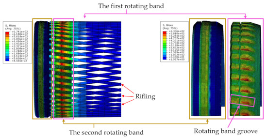
Figure 13.
Appearance and stress distribution of the rotating bands and riflings in the first period.
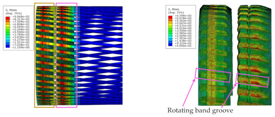
Figure 14.
Appearance and stress distribution of the rotating bands and riflings in the second period.
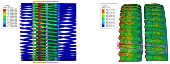
Figure 15.
Appearance and stress distribution of the rotating bands and riflings in the third period.
In the first period, the initial segments of 48 riflings are cutting the first rotating band. Thus, the high stress produces plastic and damage deformation of the first rotating band, so the corresponding 48 rotating band grooves form, and the rotating bands begin to rotate. As for the second rotating band, it is squeezed by the bore surface and also undergoes plastic deformation, as shown in the brown wireframe in Figure 13. Hence, the second rotating band can avoid the spillage of the propellant gas.
In the second period, the initial segments of 48 riflings are continuously cutting these two rotating bands. Since the height of initial segments of riflings gradually increases, so the depth of grooves at the first rotating band is deeper than that at the second rotating band, as exhibited in Figure 14.
In the third period, the initial segments of 48 riflings have cut these two rotating bands completely, and the whole engraving process finishes. After the engraving process, no obvious changes in groove shape will take place until the rotating bands and projectile leave the muzzle.
The engraving resistance force is calculated by Equation (9), and its value is shown in Figure 16a. Here s is the projectile base area, is the projectile base pressure, which is calculated by the launch-load model, m is the projectile mass, a is the projectile acceleration, which is simulated by Abaqus explicit solver.
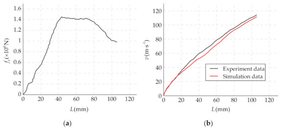
Figure 16.
(a) Engraving resistance force vs. projectile displacement; (b) engraving-completion velocity of the projectile vs. projectile displacement.
Figure 16b shows engraving-completion velocity data of the projectile, which is simulated by Abaqus explicit solver. As can be seen, the engraving-completion velocity of the projectile by simulation is 111.46 m∙s−1, and that by the experiment is 114.13 m∙s−1. Compared with the data, the error is −2.58%. Therefore, the accuracy of the finite element model is validated.
From the above simulation results of the finite element model, the interaction between rotating bands, riflings and bore surface produces cut phenomenon and squeezing phenomenon, which complete the engraving functions. On the other hand, the cut and squeezing phenomenon also generates the engraving resistance force, which is opposite to the direction of the propellant gas force and will impede the projectile motion. Because the smaller the engraving resistance force is, the higher engraving-completion velocity and the higher muzzle velocity are. So, the engraving resistance force is the third performance evaluation index during the engraving process. Furthermore, the size parameters of the gun engraving system have an effect on the engraving resistance force and the motion state of the projectile. Subsequently, by determining the space volume of the propellant combustion, the state of the projectile motion can also affect the temperature value and the pressure wave value of the propellant gas. In conclusion, the size parameters of the gun engraving system have an effect on all three performance evaluation indexes, and it is necessary to optimize size parameters for better performance.
3. Sensitivity Analysis of Size Parameters of the Gun Engraving System
3.1. The Meaning and Range of Size Parameters
In the optimal design process, the less modification and the more performance improvement are pursued by designers. Therefore, before optimization, sensitivity analysis of size parameters of the gun engraving system is needed and will be carried out in this section. Figure 17 and Figure 18 present the meanings of size parameters from to . Additionally is the forcing cone angle. The nominal values and tolerance intervals of size parameters are listed in Table 4.
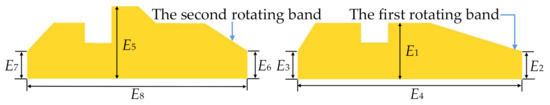
Figure 17.
Schematic diagram of the position of size parameters on the cross profile of the rotating bands.

Figure 18.
Schematic diagram of the position of size parameters on the initial segment of rifling.
Table 4.
The nominal values and tolerance intervals of size parameters.
3.2. The Method and Process of Sensitivity Analysis
The sensitivity analysis process denoted in Figure 19 is illustrated as follows:
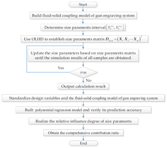
Figure 19.
Flow chart of the sensitivity analysis process.
Step 1: the fluid–solid coupling model of the gun engraving system is built.
Step 2: the upper limits and lower limits of the twelve size parameters are determined, respectively.
Step 3: the size parameters matrix is obtained by the OLHD (optimal Latin hypercube design) methods [33].
Step 4: the size parameters matrix is brought into the fluid–solid coupling model of the gun engraving system until the end of the simulation.
Step 5: the polynomial regression model is employed to reflect the response relationship of the gun engraving system model, as follows:
The unknown parameter can be estimated by ordinary least squares. The principle is to minimize the sum of the squares of the residuals:
This least-squares method should satisfy the equation . The partial derivative of Equation (11) is set to 0:
The equivalent form of Equation (12) is expressed as follows:
The matrix operation method is adopted to solve the normal Equation (13):
According to the operation rules of the matrix, Equation (12) can be expressed as a matrix form:
Then, Equation (16) can be obtained by left multiplying :
Step 6: Since the parameters are normalized before analysis, the fitted model coefficients can fairly reflect the contribution of input variables to the response. The coefficients of the polynomial regression model are transformed into contribution ratio by Equation (17):
Step 7: In order to better characterize the contribution rate of each parameter, the sensitivity results on the performance evaluation indexes T, , are taken as absolute values. The comprehensive contribution ratio is expressed by Equation (18):
3.3. The Results of Sensitivity Analysis
As described in Figure 8, there are totally three performance evaluation indexes during the engraving process. Figure 20a–c show sensitivity analysis results on these three performance evaluation indexes, respectively, and Figure 20d shows sensitivity analysis results on the comprehensive performance index. In Figure 20d, the dotted line is a separate line whose contribution rate is 10%. Moreover, the size parameters whose contribution rate is more than 10% are defined as high-influence size parameters. As can be seen, the contribution rates of , , and are more than 10%, and so these four size parameters are taken as design variables for optimization in Section 5.
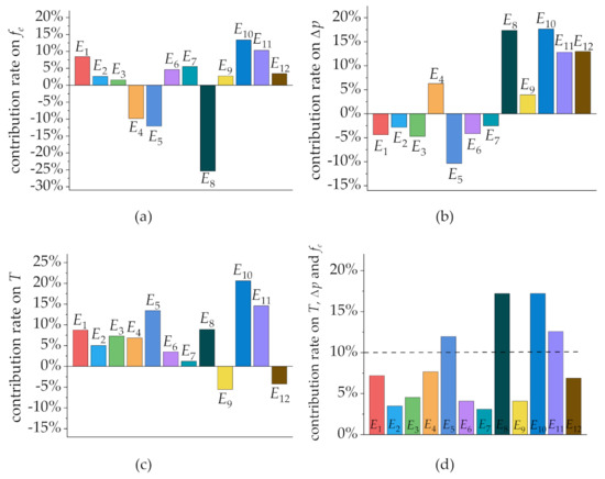
Figure 20.
Sensitivity analysis results on (a) engraving resistance force (b) pressure wave of the propellant gas (c) propellant gas temperature (d) three performance evaluation indexes.
4. The Interval Uncertain Optimization Method Based on Affine Arithmetic
4.1. Nonlinear Interval Uncertain Optimization Problem
The nonlinear interval uncertain optimization can be expressed as follows [16]:
where X is the n-dimensional design vector whose value range is .U is a q-dimensional uncertain vector, which is described by a q-dimensional interval vector . f and are objective function and the i-th constraint, respectively. For the optimization model of the gun engraving system, the engraving resistance force is taken as an objective function. Because can affect the engraving-completion velocity of the projectile. Moreover, the engraving-completion velocity of the projectile is the most crucial index for designers. Additionally, the temperature of the propellant gas T can affect the erosion degree and service life of the gun barrel. The pressure wave of the propellant gas can affect the propellant combustion stability. Both T and should be in a feasible scope. Therefore, T and are taken as a constraint. l is the number of constraints. They are all continuous nonlinear functions of X and U, and at least one of them is a nonlinear function of U. is the allowable interval of the i-th uncertain constraint, and it can also be a real number in practical problems.
Since the objective function and the constraint are both continuous functions of U, for any design variable X that is determined, the values of the objective function and the constraint are also intervals.
4.2. Affine Arithmetic
In interval arithmetic, two interval numbers are set as ,, and the basic operation rules are as follows:
The interval arithmetic can directly calculate the interval number. Although the calculation is simple, it will bring about the interval expansion phenomenon. When calculating the function value range, the calculation result interval is amplified. For example, calculate , where . The resulting interval obtained from Equation (19) is , while the actual result is . The root of the interval expansion problem comes from the correlation between interval numbers.
The affine arithmetic is similar to interval arithmetic, but the affine arithmetic considers the correlation of variables in the calculation, so it can well suppress the interval expansion. Moreover, when the same variable appears in different terms of the function, the affine arithmetic can retain its complete correlation to the greatest extent, while the interval arithmetic will cause serious information loss. The affine form of the uncertain quantity is denoted as :
where is the central value of the affine afform, and the are noise symbols, whose values are unknown but definitely lie in the interval [−1, 1], correspondingly, are the known real coefficients of the noise symbols. When , the affine form obtains its maximum and minimum values, which can be expressed as the interval:
For interval uncertain optimization problems, the uncertain interval quantity can be expressed as:
where and are the central value and radius of the interval, respectively.
Affine afform and :, The basic affine operation rules are as follows:
The quadratic term appears in the multiplication operation. can be obtained from , so the upper and lower bounds of the affine operation can be expressed as interval , where:
4.3. An Optimization Method Based on Affine Arithmetic
In this work, a nonlinear interval uncertain optimization method based on affine arithmetic is adopted, and the phrase “affine arithmetic-based method” is used for calling this method. First, the uncertain variables in the objective function and constraint are rewritten into the affine form. Second, the affine arithmetic is utilized to obtain the interval of objective function and constraint of the design variable X, and then the uncertain problem is transformed into a deterministic problem. Finally, the genetic algorithm is used to solve the problem.
The details of the approach are summarized below.
First, let . Then, the objective function is rewritten into affine form.
where is the central value of the affine form, are the known real coefficient, are the noise symbol. Therefore, the interval of the objective function at the design variable can be obtained:
Second, the constraints are rewritten in affine form:
where is the central value of the affine form, are the known real coefficient, are the noise symbol. The interval of the constraint at the design variable can be obtained:
The above uncertain problem can be rewritten as:
It can be further rewritten as:
At this point, the uncertain optimization problem is transformed into a single-layer deterministic optimization problem, which can be solved by existing sequential quadratic programming (SQP), genetic algorithm (GA) and other intelligent optimization algorithms. This method is further illustrated with a numerical example below.
This numerical example is a nonlinear interval optimization problem with three uncertain variables, and it is from a doctoral thesis [34]. In addition, all the parameters, which we set, are the same as the parameters in reference [34].
Step 1: rewriting the interval quantity into affine quantity.
Let ,,.
Step 2: computing the affine form of the objective function.
The nonlinear term of the uncertain variables in the objective function are and:
The objective function can be rewritten as:
Since, the value interval of even term are . The interval of the objective function can be obtained as:
Step 3: computing the affine form of the constraints.
The nonlinear term of the uncertain variables in the objective function are and :
The constraint can be rewritten as:
Since , the value interval of even term is . The interval of constraint can be obtained as:
Similarly, the affine form of the constraint can be obtained as:
Its value interval is:
Step 4: deterministic transformation.
The original uncertain optimization problem can be rewritten as the optimization problem in the following affine form:
According to the interval order model proposed in Reference [16], the above optimization problem can be transformed into the following deterministic optimization problem:
So far, the nonlinear interval uncertainty optimization problem has been transformed into a deterministic optimization problem. The linear weighting method can be used to further convert the problem into a single-objective optimization problem:
where is the multiobjective evaluation function, is the multiobjective weight coefficient,is the parameter that guarantees and to be nonnegative,andare regularization factors of a multiobjective function.
In order to be consistent with reference [34], the regularization factors,andare 1.33, 0.34 and 0.0, respectively. GA [35] is used to solve the problem, and the results are listed in Table 5.
Table 5.
Comparison of optimization results.
The calculation results obtained by the two-layer nested method are regarded as the reference solution for interval uncertain optimization problem. Comparing with the results by these two methods, the max error is only 1.6%. It indicates that the affine arithmetic-based method has high accuracy. Furthermore, the affine arithmetic-based method costs only 1.944 s to complete the numerical example, while the two-layer nested method costs 544.48 s. It also indicates that the affine arithmetic-based method has obvious improvement in computational efficiency.
5. Uncertain Optimization of the Gun Engraving System
5.1. Optimization Model
As described in Figure 8, there are totally three performance evaluation indexes during the engraving process. Because the engraving-completion velocity of the projectile is the most crucial index for designers, thus the engraving resistance force is taken as the objective function. Additionally, the temperature T and the pressure wave of the propellant gas are taken as constraints.
The optimization model of the gun engraving system, which is as expressed in Equation (44), contains four design variables, namely the rifling width , the rifling height , the total height of the second rotating band , the width of the second rotating band . In addition, four uncertain parameters, namely the propellant length, the propellant thickness, the projectile mass, the propellant mass, are taken into consideration.
According to the interval order model [16], the uncertain optimization model above is converted into a deterministic multiobjective optimization model shown as follows:
The model cannot be directly processed by the affine arithmetic. Therefore, the response surface method (RSM) [36] is employed to construct the explicit polynomial expressions of the objective function and constraint. Thereby, the intervals of objective functions and constraints can be obtained by affine arithmetic. Finally, the uncertain problem is transferred into a deterministic problem that can be easily solved.
5.2. Optimization Results
The NSGA-II [37] exhibits good global convergence without falling into the local optima and has strong robustness, which is especially suitable for multiobjective optimization problems. Therefore, it is used as the optimization operator. The population size is set as 100, and the stopping criterion is set as 100 generations. Finally, the Pareto front is obtained, as shown in Figure 21.
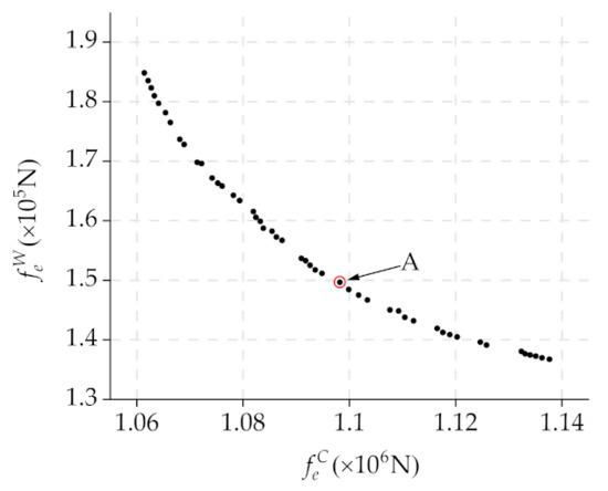
Figure 21.
The Pareto front of optimization results.
All solutions in the Pareto front are feasible. The choice of the final solution depends on the preference of the decision-maker. Optimizing is for improving the average design performance of an objective function under uncertainty. Minimizing can reduce the sensitivity of the objective function to uncertainty, and thereby can ensure design robustness. Therefore, considering both the average design performance and the robustness, the “A” point in Figure 21 is adopted as the final optimal solution. The corresponding size parameters data are listed in Table 6.
Table 6.
Comparison of design variables before and after optimization.
Finally, by substituting the optimized size parameters data into the model of the gun engraving system, the initial and optimized interval of performance evaluation indexes are obtained, as shown in Figure 22,Figure 23,Figure 24. Additionally, the detailed performance evaluation indexes of point A are listed in Table 7. As can be seen, after optimization, decreases, and the percent decrease of ranges from 6.34% to 18.24%. T also decreases, and the percent decrease of ranges from 1.91% to 7.45%. At the same time, the change of is not obvious and the percent increase of ranges slightly from 0.12% to 0.36%. The optimization results mean that, first, the engraving-completion velocity of the projectile raises. Then the erosion degree of the gun barrel declines during the engraving process, and the service life of the gun barrel improves. Finally, the combustion stability of the propellant has no obvious change.

Figure 22.
The initial and optimized interval of the engraving resistance force.
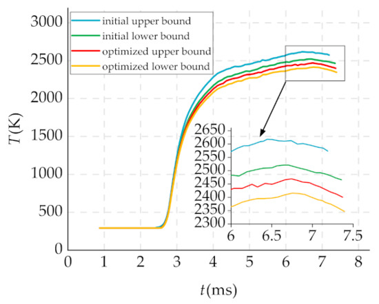
Figure 23.
The initial and optimized interval of the propellant gas temperature.
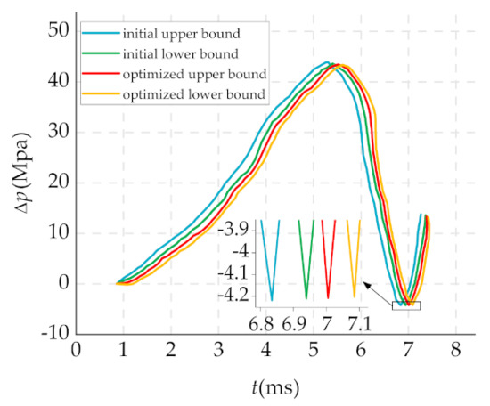
Figure 24.
The initial and optimized interval of pressure wave of the propellant gas.
Table 7.
Detailed performance evaluation indexes of point A.
6. Conclusions
In this paper, first, a computational model of the launch load and the finite element model of the gun engraving system was established and validated by the gun launch experiment. Then by solving the launch-load model, two performance evaluation indexes, namely the propellant gas temperature and the pressure wave of the propellant gas, were obtained. By solving the finite element model, the engraving resistance force, as the third performance evaluation index, was obtained. Second, the sensitivity analysis was performed, and four high-influence size parameters were selected as design variables. Finally, an interval uncertain optimization method based on affine arithmetic was introduced and validated by the numerical example. The validation results showed this method had high accuracy and high computational efficiency. Then the uncertain optimization on three performance evaluation indexes was carried out. From the simulation results and optimization results, two main conclusions can be drawn:
- 1.
- During the engraving process, the projectile rotating bands are squeezed by the bore surface and cut by riflings, which will lead to the plastic deformation and damage of the rotating bands. The functions of this process are making the projectile rotate and avoiding the spillage of the propellant gas. On the other hand, the cut and squeezing process also generates the engraving resistance force, which will impede the projectile motion. By the mechanism analysis of the engraving process, twelve related size parameters are selected for the sensitivity analysis
- 2.
- After the optimal design of size parameters of the gun engraving system, the percent decrease of maximum engraving resistance force ranges from 6.34% to 18.24%, which means an increase of the engraving-completion velocity of the projectile. The percent decrease of maximum propellant gas temperature ranges from 1.91% to 7.45%, which means the improvement in erosion degree and service life of the gun barrel. The percent increase of the minimum pressure wave of the propellant gas ranges from 0.12% to 0.36%, which means that the combustion stability of the propellant has no obvious effect.
The present work provides an optimal design scheme with high-efficiency and low-cost. It would be suitable for not only gun engraving systems but also other industrial products.
Author Contributions
T.X. wrote the framework of the paper. G.Y. reviewed and validated the paper. F.X. supplied the optimization model. Q.S. helped to carry out the experiment. A.M. checked the grammar and develop the program. All authors have read and agreed to the published version of the manuscript.
Funding
This research was funded by the National Natural Science Foundation of China, grant number 11572158 and 51705253.
Institutional Review Board Statement
Not applicable.
Informed Consent Statement
Not applicable.
Data Availability Statement
Not applicable.
Conflicts of Interest
The authors declare no conflict of interest.
References
- Wu, B.; Fang, L.H.; Zheng, J.; Yu, X.H.; Jiang, K.; Wang, T.; Hu, L.M.; Chen, Y.L. Strain Hardening and Strain-Rate Effect in Friction Between Projectile and Barrel During Engraving Process. Tribol. Lett. 2019, 67, 1–8. [Google Scholar] [CrossRef]
- Wu, B.; Zheng, J.; Tian, Q.-t.; Zou, Z.-q.; Chen, X.-l.; Zhang, K.-s. Friction and wear between rotating band and gun barrel during engraving process. Wear 2014, 318, 106–113. [Google Scholar] [CrossRef]
- Wu, B.; Zheng, J.; Tian, Q.-t.; Zou, Z.-q.; Yu, X.-h.; Zhang, K.-s. Tribology of rotating band and gun barrel during engraving process under quasi-static and dynamic loading. Friction 2014, 2, 330–342. [Google Scholar] [CrossRef]
- Wu, B.; Fang, L.-h.; Chen, X.-l.; Zou, Z.-q.; Yu, X.-h.; Chen, G. Fabricating Aluminum Bronze Rotating Band for Large-Caliber Projectiles by High Velocity Arc Spraying. J. Therm. Spray Technol. 2013, 23, 447–455. [Google Scholar] [CrossRef]
- Wu, B.; Zheng, J.; Qiu, J.; Zou, Z.-q.; Yan, K.-b.; Chen, X.-l.; Hu, L.-m.; Zhang, K.-s.; Chen, R.-g. Preparation of the projectile rotating band and its performance evaluation. Adhes. Sci. Technol. 2016, 30, 1143–1164. [Google Scholar] [CrossRef]
- Sudarsan, N.V.; Sarsar, R.B.; Das, S.K.; Naik, S.D. Prediction of Shot Start Pressure for Rifled Gun System. Def. Sci. J. 2018, 68, 144–149. [Google Scholar] [CrossRef]
- Sun, Q.; Yang, G.; Ge, J. Modeling and simulation on engraving process of projectile rotating band under different charge cases. J. Vibrat. Control. 2016, 23, 1044–1054. [Google Scholar] [CrossRef]
- Monreal-González, G.; Otón-Martínez, R.A.; Velasco, F.J.S.; García-Cascáles, J.R.; Ramírez-Fernández, F.J. One-Dimensional Modelling of Internal Ballistics. J. Energ. Mater. 2017, 35, 397–420. [Google Scholar] [CrossRef]
- Monreal-González, G.; Otón-Martínez, R.A.; Velasco, F.J.S.; García-Cascales, J.R.; Moratilla-Fernández, D. A one-dimensional code for the analysis of internal ballistic problems. In Proceedings of the 28th International Symposium on Ballistics, Atlanta, GA, USA, 22–26 September 2014. [Google Scholar]
- Otón-Martínez, R.A.; Monreal-González, G.; García-Cascales, J.R.; Vera-García, F.; Velasco, F.J.S.; Ramírez-Fernández, F.J. An approach formulated in terms of conserved variables for the characterisation of propellant combustion in internal ballistics. Int. J. Numer. Methods Fluids. 2015, 79, 394–415. [Google Scholar] [CrossRef]
- López, M.; García, C.; Velasco; Otón, M. An Energetic Model for Detonation of Granulated Solid Propellants. Energies 2019, 12, 4459. [Google Scholar] [CrossRef]
- Wang, S.; Yao, Y.; Long, X. Critical review of size effects on microstructure and mechanical properties of solder joints for electronic packaging. Appl. Sci. 2019, 9, 227. [Google Scholar] [CrossRef]
- Cavas, F.; Pinero, D.; Velazquez, J.S.; Mira, J.; Alio, J.L. Relationship between Corneal Morphogeometrical Properties and Biomechanical Parameters Derived from Dynamic Bidirectional Air Applanation Measurement Procedure in Keratoconus. Diagnostics 2020, 10, 640. [Google Scholar] [CrossRef]
- Luhandjula, M.K. Fuzzy optimization: Milestones and perspectives. Fuzzy Sets Syst. 2015, 274, 4–11. [Google Scholar] [CrossRef]
- Jiang, C.; Han, X.; Liu, G.P. A sequential nonlinear interval number programming method for uncertain structures. Comput. Meth. Appl. Mech. Eng. 2008, 197, 4250–4265. [Google Scholar] [CrossRef]
- Jiang, C.; Han, X.; Liu, G.R.; Liu, G.P. A nonlinear interval number programming method for uncertain optimization problems. Eur. J. Oper. Res. 2008, 188, 1–13. [Google Scholar] [CrossRef]
- Chen, S.H.; Wu, J.; Chen, Y.D. Interval optimization for uncertain structures. Finite Elem. Anal. Des. 2004, 40, 1379–1398. [Google Scholar] [CrossRef]
- Li, Y.; Xu, Y.L. Increasing accuracy in the interval analysis by the improved format of interval extension based on the first order Taylor series. Mech. Syst. Signal. Proc. 2018, 104, 744–757. [Google Scholar] [CrossRef]
- Zhou, J.; Li, M. Advanced Robust Optimization With Interval Uncertainty Using a Single-Looped Structure and Sequential Quadratic Programming. J. Mech. Des. 2014, 136, 021008. [Google Scholar] [CrossRef]
- Wu, J.; Zhang, Y.; Chen, L.; Luo, Z. A Chebyshev interval method for nonlinear dynamic systems under uncertainty. Appl. Math. Model. 2013, 37, 4578–4591. [Google Scholar] [CrossRef]
- Wang, L.; Chen, Z.; Yang, G. An interval uncertainty analysis method for structural response bounds using feedforward neural network differentiation. Appl. Math. Model. 2020, 82, 449–468. [Google Scholar] [CrossRef]
- Wang, L.; Chen, Z.; Yang, G.; Sun, Q.; Ge, J. An interval uncertain optimization method using back-propagation neural network differentiation. Comput. Meth. Appl. Mech. Eng. 2020, 366, 113065. [Google Scholar] [CrossRef]
- Luque, M.; Marcenaro-Gutierrez, O.D.; Ruiz, A.B. Evaluating the global efficiency of teachers through a multi-criteria approach. Socio-Econ. Plan. Sci. 2020, 70, 100676. [Google Scholar] [CrossRef]
- Ruiz, A.B.; Saborido, R.; Bermúdez, J.D.; Luque, M.; Vercher, E. Preference-based evolutionary multi-objective optimization for portfolio selection: A new credibilistic model under investor preferences. J. Glob. Optim. 2019, 76, 295–315. [Google Scholar] [CrossRef]
- Luque, M.; Gonzalez-Gallardo, S.; Saborido, R.; Ruiz, A.B. Adaptive Global WASF-GA to handle many-objective optimization problems. Swarm Evol. Comput. 2020, 54, 100644. [Google Scholar] [CrossRef]
- Luque, M.; Ruiz, A.B.; Saborido, R.; Marcenaro-Gutiérrez, Ó.D. On the use of the Lp distance in reference point-based approaches for multiobjective optimization. Ann. Oper. Res. 2015, 235, 559–579. [Google Scholar] [CrossRef]
- Cavas Martinez, F.; Garcia Fernandez-Pacheco, D. Virtual Simulation: A technology to boost innovation and competitiveness in industry. Dyna 2019, 94, 118–119. [Google Scholar] [CrossRef]
- Ruiz, L.; Torres, M.; Gómez, A.; Díaz, S.; González, J.M.; Cavas, F. Detection and Classification of Aircraft Fixation Elements during Manufacturing Processes Using a Convolutional Neural Network. Appl. Sci. 2020, 10, 6856. [Google Scholar] [CrossRef]
- Velázquez, J.S.; Cavas, F.; Bolarín, J.M.; Alió, J.L. 3D Printed Personalized Corneal Models as a Tool for Improving Patient’s Knowledge of an Asymmetric Disease. Symmetry 2020, 12, 151. [Google Scholar] [CrossRef]
- Luo, Q.; Zhang, X. Numerical simulation of gas-solid two-phase reaction flow with multiple moving boundaries. Int. J. Numer. Methods Heat Fluid Flow 2015, 25, 375–390. [Google Scholar] [CrossRef]
- Jaramaz, S.; Micković, D.; Elek, P. Two-phase flows in gun barrel: Theoretical and experimental studies. Int. J. Multiph. Flow. 2011, 37, 475–487. [Google Scholar] [CrossRef]
- MacCormack, R. The effect of viscosity in hypervelocity impact cratering. In Proceedings of the 4th Aerodynamic Testing Conference, Cincinnati, OH, USA, 28–30 April 1969; American Institute of Aeronautics and Astronautics: Reston, VA, USA, 1969. [Google Scholar]
- Park, J.-S. Optimal Latin-hypercube designs for computer experiments. J. Stat. Plan. Infer. 1994, 39, 95–111. [Google Scholar] [CrossRef]
- Chao, J. Theories and algorithms of uncertain optimization based on interval. Doctoral Thesis, Hunan University, Changsha, China, 2008. [Google Scholar]
- Whitley, D. A genetic algorithm tutorial. Stat. Comput. 1994, 2, 65–85. [Google Scholar] [CrossRef]
- Wang, G.G.; Shan, S. Review of Metamodeling Techniques in Support of Engineering Design Optimization. J. Mech. Des. 2007, 129, 370–380. [Google Scholar] [CrossRef]
- Deb, K.; Pratap, A.; Agarwal, S.; Meyarivan, T. A fast and elitist multiobjective genetic algorithm: NSGA-II. IEEE Trans. Evol. Comput. 2002, 6, 182–197. [Google Scholar] [CrossRef]


Publisher’s Note: MDPI stays neutral with regard to jurisdictional claims in published maps and institutional affiliations. |
© 2021 by the authors. Licensee MDPI, Basel, Switzerland. This article is an open access article distributed under the terms and conditions of the Creative Commons Attribution (CC BY) license (http://creativecommons.org/licenses/by/4.0/).