2.1. Stringing via Manifold Learning
Let be the data consisting of n samples with associated responses . The exponent “” indicates the transpose. The p predictors , , are n-dimensional vectors that can be arranged in an design matrix: with elements , . Each represents the observed value of the predictor j for subject i. We consider a high-dimensional scenario with many predictors and possibly , also known as “wide data” (opposed to “tall data”). The vector gathers all the responses. In what follows, bold-upper-case letters will indicate a matrix (e.g., design matrix ) or a column vector (e.g., the vector of responses or the j-th column of : ). Bold-lower-case letters will indicate row vectors (e.g., the i-th row of : ). A tilde over a matrix () indicates that the columns are scrambled in a random way.
Following [
1], we consider stringing as a class of methods that map the samples (
) from
to the infinite space of square-integrable functions
defined over a closed interval
. We consider data as realizations of a hidden smooth stochastic process (say
), but observed in random order of its components. This means that for each subject
, we observe
p realizations
, where
is an unknown node to be estimated.
The main goal of stringing is to estimate positions to each predictor indexed by . In other words, to recover the true order of the nodes generating the observations, as well as their positions in a closed interval . In practice, stringing addresses the problem by reducing the dimension of the predictors from n to , while preserving dissimilarities across spaces.
Our proposal, stringing via ML, aims to preserve more complex relations between predictors, as nonlinearities. Therefore, we assume that the predictors
(columns of the design matrix
) are the result of mapping the coordinates
of an underlying
l-dimensional smooth manifold
. Following [
16], and avoiding the complexities regarding the definition of a topological manifold, we consider
as a space that locally behaves like Euclidean space. We consider that
is continuously differentiable (i.e., smooth), connected, and equipped with a metric
that determines its structure. This metric is usually called geodesic distance, as it is the arc-length of the shortest curve connecting any two points in the manifold.
In this paper, the dimension of
is fixed to
, which makes ML analogous to UDS. We focus on six ML and Nonlinear Dimensionality Reduction algorithms:
Isometric Feature Mapping (Isomap) [
17],
Locally Linear Embedding (LLE) [
18],
Laplacian Eigenmap (LaplacianEig) [
19],
Diffusion Maps (DiffMaps) [
20],
t-Distributed Stochastic Neighbor Embedding (tSNE) [
21], and
Kernel Principal Component Analysis (kPCA) [
22]. In general, the ML algorithms start by constructing a weighted graph that considers neighborhood information between the sample objects (e.g., the predictors in stringing). Then, the weighted graph is transformed according to a certain criterion that is particular to each algorithm. Finally, the data is embedded into a lower-dimensional space, commonly by solving an eigen equation problem.
Isomap starts by joining neighboring points, defined as the -nearest according to the Euclidean distance in . Then it approximates the geodesic distances in the underlying manifold by computing the shortest paths that connect any two points . The third and final step uses the approximations as inputs of an MDS algorithm.
For any set of dissimilarities
, MDS estimates the minimizing
of the
stress:
where
means
monotonically related quantities (
for all
); and the
represent point-to-point distances of a configuration
. Details regarding the estimation of optimal
can be found in [
16,
23].
On the one hand, Isomap can be seen as an extension of MDS that attempts to preserve the global geometry of . As it estimates all the geodesic distances in the underlying manifold, it is a global approach to the ML problem.
On the other hand, the LLE algorithm is seen as a local approach because it preserves local neighborhood information without approximating all the
. First, for a fixed number of neighbors
, it reconstructs each point
through a linear combination of its
-nearest neighbors
:
with weights
minimizing the reconstruction error:
The coordinates
, best reconstructed by the weights
, are estimated by minimizing the
embedding cost function:
Under some constraints that make the objective function invariant under translation, rotation, and change in scale, the problem is reduced to the estimation of the bottom
eigenvectors of the sparse
matrix
. The “bottom” eigenvectors refer to those with the
smallest eigenvalues,
is the identity matrix of size
, and
is the matrix of optimal weights
.
The Laplacian Eigenmap algorithm is very similar to the previous two. It starts by defining the
-neighborhoods
of each data point
, as in LLE or Isomap algorithms. Next, a weighted adjacency matrix
is constructed, according to:
with weights determined by the
isotropic Gaussian kernel. The parameter
can also take the value infinity (
), resulting in the
simple-minded version:
, if
and 0, otherwise. This results in a graph
, with connected neighboring points and weights given by
. Let
be the
degree matrix, meaning it is a diagonal matrix with nonzero elements:
Then, the
graph Laplacian of
is the
, symmetric, and positive semidefinite matrix
. The coordinates
are determined by the solution of the optimization problem:
This is simplified to solving the generalized eigen equation
, or, equivalently, computing the bottom
eigenvalues and eigenvectors of
.
Diffusion Maps are a very interesting alternative to ML. They exploit the relationship between
heat diffusion and
Markov chains, based on the idea that it is more likely to visit nearby data-points while taking a random walk through the data. The algorithm departs from the same weights matrix
, with entries defined in Equation (
2), as in Laplacian Eigenmaps. Using both
and
, the degree matrix with diagonal elements defined in Equation (
3), the algorithm calculates the
random walk transition matrix . The elements of
give a sense of connectivity between
and
. By analogy with random walks,
represents the probability for a single step taken from
i to
j. Moreover, the iterative matrix
gives the transition probabilities on the graph after
t time steps. The coordinates of the embedding are obtained by solving the eigen equation
and retaining the top
eigenvectors and eigenvalues.
The tSNE algorithm is a variant of the
Stochastic Neighbor Embedding (SNE) [
24] that improves the original approach by introducing a Student t-Distribution as a kernel in the target low-dimensional space. tSNE first constructs a probability distribution over the high-dimensional data space:
with
and
. One can understand the similarity between data points
as the conditional probability,
, that
would pick
as its neighbor. Next, we define the the joint probabilities
in the high-dimensional space to be the symmetrized conditional probabilities, i.e.:
The
bandwidth of the Gaussian kernel defining the probabilities in Equation (
4) is set in such a way that the
perplexity of the conditional distribution (i.e., a measurement of how well the probability distribution predicts the sample) equals a predefined value. Briefly,
is adapted to the density of the data, were smaller values are used in denser parts of the data space. The similarities between the coordinates
in the target
l-dimensional manifold
, are measured using a heavy-tailed Student t-Distribution:
with
and
. The locations are estimated by minimizing the
Kullback–Leibler divergence (KL) of the distribution
P from the distribution
Q using gradient descent:
kPCA is a nonlinear version of PCA that applies the well-known
kernel trick. It can be seen as a two-steps process where: (1) each
is nonlinearly transformed into
, where
is an
-dimensional Hilbert space; and (2) given the
with
, solve a linear PCA in
feature space . The
feature map is such that:
with
and nonlinear maps
. The idea behind the method is that any possible low-dimensional structure of the data can be more easily seen in a much higher-dimensional space. Also, the feature map does not need to be defined explicitly.
Briefly, solving a linear PCA in feature space mimics a standard PCA. The goal is to find eigenvalues
and nonzero eigenvectors
of the covariance matrix:
of the centered and nonlinearly transformed input vectors. In practice, the eigenvalues and eigenvectors
of
are expressed in terms of the eigenvalues and eigenvectors
of the matrix
with elements:
where the inner product
in
is substituted by a feasible kernel
. The principal components
are not computed explicitly. Instead, for any point
, its nonlinear principal component scores corresponding to
are given by the projection of
onto the eigenvectors
, using the kernel trick:
for
. Please note that the
are obtained from the ordered eigenvalues of
:
, with associated eigenvectors
, such that
.
In any case, the estimated order of the predictors is characterized with a permutation
, called the
stringing function [
1], such that
. Also, for each predictor
j with rank order
and for a fixed
T, a regularized position
is computed. The purpose is to normalize the resulting domain to
, usually for
. It is worth noting that in the original stringing, the order is estimated by plugging in Equation (
1) the Euclidean distances or empirical Pearson correlations between any two columns
of the matrix
:
where
To simplify, we write UDS- and ML-stringing to allude the original method and our proposal, respectively. We also write Isomap-stringing, LLE-stringing, tSNE-stringing, etc., to refer to a particular algorithm.
In our applications we take advantage of the packages
dimRed and
coRanking [
25] in
R software [
26] to estimate the optimal one-dimensional configuration
. Please note that we are fixing
, while in most dimensionality reduction methods the usual is to estimate the
bestl. Nevertheless, while fixing
we can still enhance ML-stringing by tuning the parameters of each algorithm.
In this paper, we estimate the optimal number of neighbors (
) that improves the representation resulting from Isomap, LLE, and Laplacian Eigenmap. In particular, we choose
from a grid of possible
between 5 and
p, according to the optimal
Local Continuity Meta Criterion (LCMC) [
27]. Also, we follow the simple-minded version of Laplacian Eigenmap, meaning
in its Gaussian kernel. Diffusion Maps are set to compute the coordinates in
after a single time step (
), the parameter
in its Gaussian kernel is set to the median distance to the
nearest neighbors, according to the default specifications from
dimRed. The perplexity parameter in tSNE algorithm is set to 30,
dimRed’s default. Roughly speaking, this value is equivalent to neighborhood size. We perform kPCA only with a Gaussian kernel and a fixed bandwidth
. Whenever possible, we compare our approach with the resulting configurations from the (UDS-based)
Stringing function available in the
R package
fdapace [
28].
2.2. Scalar-on-Function Regression
Once the regularized positions
are estimated, it is possible to represent the high-dimensional data as functional. Furthermore, it is reasonable to assume that the measurements are noisy:
with independent and identically distributed (i.i.d.) errors
. The samples are assumed to be from the second order stochastic process
, continuous in quadratic mean, and with sample paths in the Hilbert space of square integrable functions
.
In any case (stringing via UDS or ML), we can associate the observed values of the process
with the corresponding response
and consider a SOF
generalized linear model. Following the notation from [
29], we write:
where
denotes an exponential family distribution with mean
and dispersion parameter
. The linear predictor
is related to the functional covariate
through a link function
. In this paper we focus on Gaussian (continuous response) and Bernoulli (binary response) distributions, which implies that the link function
is the identity or the logit transformation:
respectively. We also assume that
is a scalar and that the coefficient function
.
Of interest are all the parameters of the SOF model in Equation (
6) and the estimation of the process
, observed with noise. As the interpretability of the results is bounded to the shape of both
and
, some regularity is needed. Usually, this is achieved by expanding the coefficient function and the functional predictors in terms of a set of basis functions. We can identify two main approaches depending on the basis functions [
30]: those using (i) data-driven bases or (ii) a priori fixed bases.
Hybrid methods combining both (i) and (ii) are also possible—e.g., [
29,
31].
The first approach exploits the Karhunen–Loève expansion of the process
in terms of its
functional principal components (FPC) [
2]. Using a small number of such FPC as basis functions also allows the representation of
. Moreover, the functional regression reduces to a classical regression model in terms of the FPC
scores. We noticed that this approach is more common in the stringing literature, maybe due to the connection of the authors with the
FPC analysis through conditional expectation (PACE) method [
32].
The second one is through a basis expansion:
where
,
are parameters to be estimated and
,
are the a-priori-fixed basis functions (often splines, wavelets, or Fourier bases, and not necessarily the same for the coefficient function and the functional predictors). The numbers
directly affect the smoothness of the estimations and there are data-driven methods to select proper values (for example, cross-validation [
2]). However, tuning the number of basis functions is commonly substituted by adding a roughness penalty (
), and fixing
to be a large value. For example, when dealing with a Gaussian distribution (the outcome is continuous and
is the identity) the estimation of
can be controlled with:
where
L is a differential operator acting on
, usually set to be its second derivative:
. Similarly, a roughness penalty can be added to the estimation of the
.
Here, we follow the second approach and expand both the functional predictors and the coefficient functions using a P-splines formulation [
33,
34] based on cubic B-splines bases. We do this in a two-steps process motivated by the
penalized functional regression method [
29]: first we estimate the smooth
and then
. In any case, we follow Ruppert’s rule of thumb [
35] and fix
. The roughness penalty of the functional predictors’ expansion is chosen via generalized cross-validation. The coefficient function is estimated by fitting the model with the package
refund [
36] in
R, a computationally efficient algorithm that takes advantage of the connection to mixed models and avoids cross-validation procedures or manual selection of the penalty.
It is worth noting that the estimated
can vary across seriation algorithms that estimate different orders of the predictors. Roughly speaking, as the set of basis functions
is fixed a priori, permuting the observation nodes (the
) can change the estimated coefficients
of the basis expansion in Equation (
7). Moreover,
can also vary as it is estimated through Equation (
8), that is, it depends on the
. However, the smoothness introduced by the finite basis expansion and/or the penalization can result in similar estimated processes and coefficient functions, even for seriation algorithms with different outputs. An extreme example is that of (nearly) constant processes: no matter the order of the observed nodes, the estimated
will be essentially the same, with no impact on the estimation of
.
Finally, we remark that stringing can be applied to any high-dimensional data, even when the underlying process estimated by the method does not have a physical interpretation. The reader may have noticed that most of the applications reviewed in the Introduction deal with genetic data (SNPs or gene expression arrays), and in such cases, there is no physical interpretation of the estimated smooth process that generates the data, nor is it needed. Stringing simply maps the high-dimensional vectors into to get a visual representation of the data and to study its characteristics from an FDA perspective. The following sections study the advantages of our proposal and illustrate its versatility in a real-data application.
2.3. Simulation Studies
Here, we present two simulation studies comparing the performance of UDS- and ML-stringing in terms of the seriation quality and the accuracy of the fitted SOF regression models. We generate data from a noisy stochastic process, using as baseline the schemes from [
3,
29]. We differentiate these studies according to the nature of the response.
In Simulation 1 (continuous response), we generate the functional predictors:
where the uppercase letters
Z and
U represent random variables distributed as
and
, respectively. The function
introduces a noisy component to the functional regressor; it is generated as
, for every fixed
. The random curves
are generated as:
where
.
Analogously, when the response is binary (Simulation 2) we generate the functional predictors:
where
and
. All the terms are generated as in Equation (
9), except for
and
.
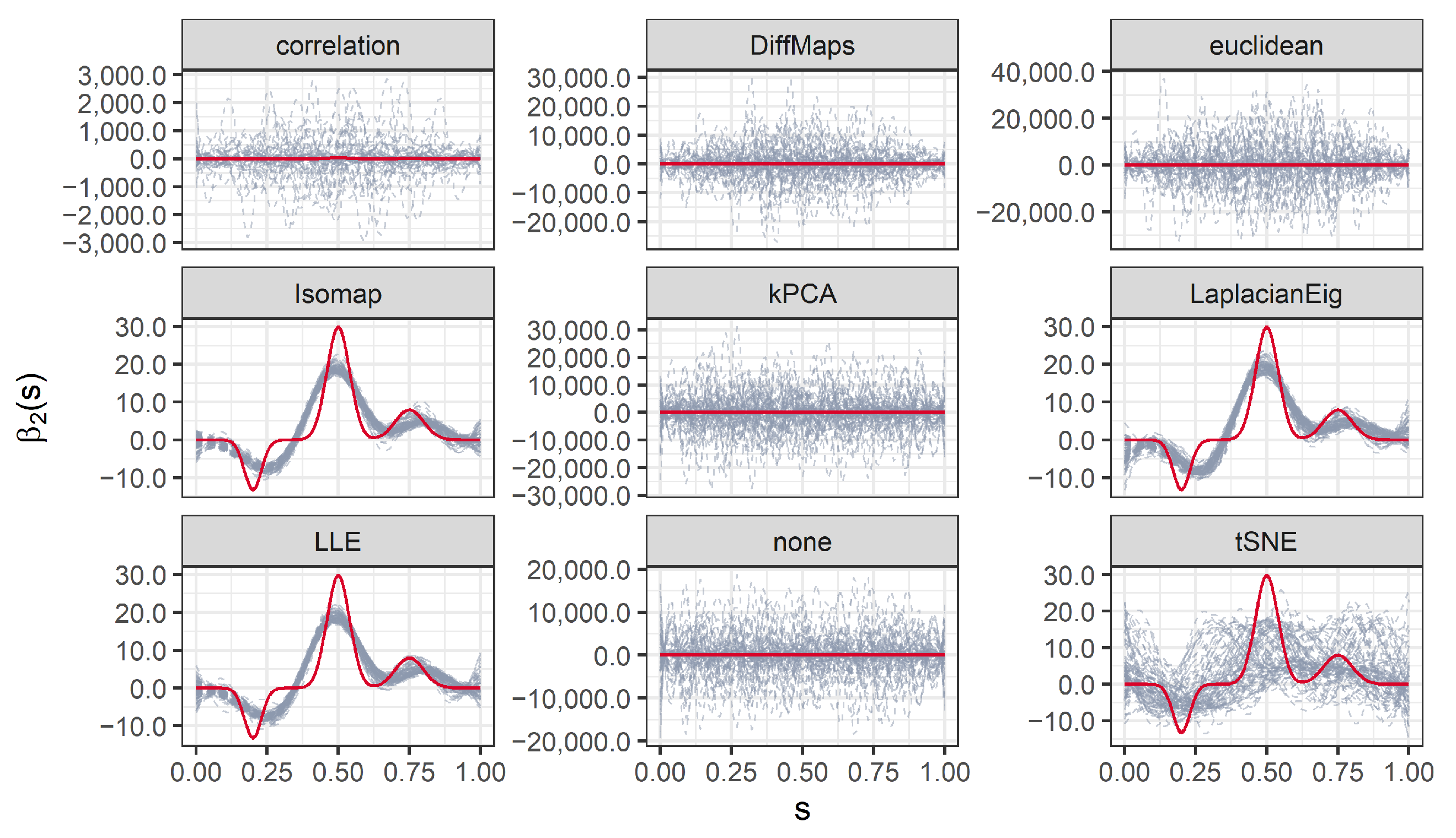
We consider two different coefficient functions
, defined over the interval
:
where
, and
are normal density functions defined by the
-duplets:
,
, and
, respectively.
Figure 1 depicts both coefficient functions.
The continuous responses (Simulation 1) are computed through the integration of:
for
and subscript
indicating which coefficient function is used. The binary responses (Simulation 2) are computed according to the functional logistic regression model, i.e.:
where
defines the probability of getting a response 1, given the functional data:
with the scalar
set to 0.
Figure 2 represents three of the generated functional predictors and their associated responses (continuous or binary) for
.
In practice each curve is evaluated over a fine grid of equally spaced knots
,
. Therefore, the realizations
, where
and
, can be arranged in a design matrix
. Then, following the hypotheses of the stringing methodology, we randomly permute its columns to obtain a new matrix
. This procedure mimics the effect of observing the functional samples with an unknown random order of the nodes. Thus, the goals are to retrieve a good estimation of the true order of the columns, achieve low prediction errors, and estimate coefficient functions closer to the true
. We evaluate the quality of the stringed order by computing the
relative order error (ROE), introduced by Chen et al. [
1]:
where
denotes the true order for each predictor indexed by
;
the order of predictor
j after the random permutation; and
the order induced by stringing. The quality of the predictions is evaluated through the test
mean square error (MSE) and
area under the receiver operating curve (AUC) for continuous and binary responses, respectively. The suitability of the estimated
is measured with the
integrated mean square error (IMSE):
We present the results for 200 simulated data sets that combine three different ratios . UDS-stringing uses Pearson correlation and Euclidean distance. ML-stringing deploys Isomap, LLE, Laplacian Eigenmaps, Diffusion Maps, kPCA, and tSNE algorithms. We also analyze the effect of taking a random order of the components. The sample is partitioned into subsets for training and testing purposes.
2.4. Case Study: Prognosis of Colon Cancer from Gene Expression Arrays
We apply stringing to a study comparing gene expressions in colon tissues of 40 cancer patients with 22 controls [
37]. The raw data is freely available in the package
colonCA [
38], and can be arranged in a
matrix
recording the gene expression data and a binary vector
of length 62, recording the sample status (we write
to indicate tumor,
normal). Our purpose is to illustrate the versatility of stringing (particularly, via ML) with a real high-dimensional dataset that has been widely approached from a multivariate analysis perspective.
Let us assume that a feasible smooth stochastic process can explain the (scrambled and noisy) observed values. The task is to estimate an order of the elements of
(and associated positions
), revealing smooth transitions between gene expression levels. Therefore, we apply stringing (both the UDS and the ML approaches) and estimate the functional predictors corresponding to the observed gene expressions of the patients. Next, we fit a logistic SOF regression as described in
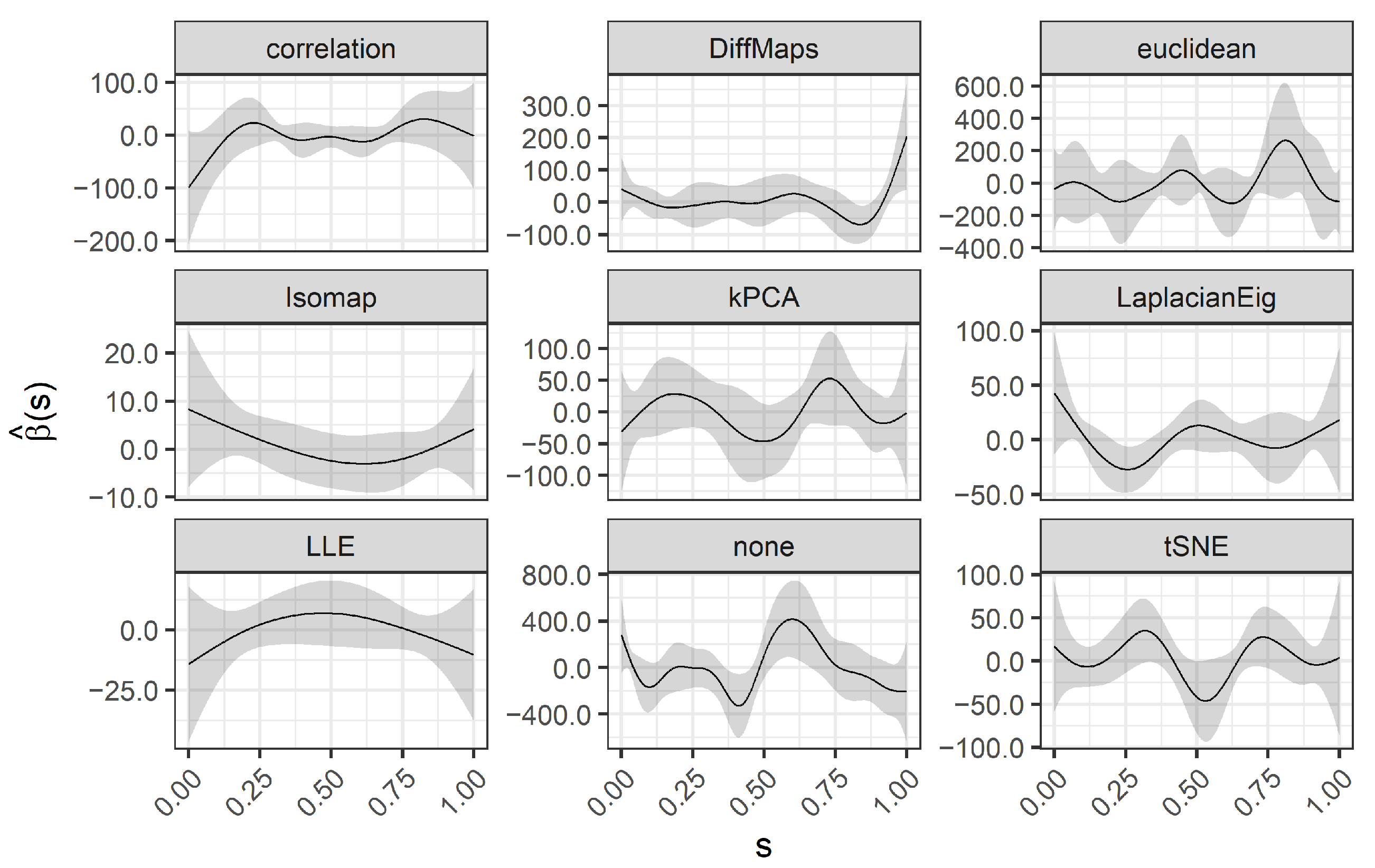
Section 2.2. We scale the data (as usual in machine learning), to obtain zero-mean columns with unit standard deviation. This step also facilitates the visual representation of the high-dimensional data.
Recall our interest in: (1) the visual representation of gene expressions achieved by the estimated functional predictors ; (2) the interpretability of the estimated coefficient function ; and (3) the accuracy of the predictions (cancer/control patients) achieved by the logistic SOF regression.
The first two aspects are strictly related to each other. In terms of interpretability, we desire smoother transitions between similar gene expression levels and an easy-to-read
(smooth, a few wiggles and sign changes). Coefficient functions act as weights of the functional predictors. Nodes
such that
indicate areas with lower impact on the outcome, while
indicates the areas that are most predictive of the outcome. In particular, estimating a
with fewer wiggles and sign changes allows an easy interpretation of the logistic SOF model in terms of
odds ratios (OR). Following [
39], we let
be the logit transformation of a specific functional observation (one of our smooth estimated processes)
, where
and
. It represents the logarithm of the odds of response
:
where
is defined as in Equation (
10). Now, let
be the logit transformation of the functional observation increased by a positive constant
A in a specific interval
. Then, it can be shown that the expression:
is an OR, so that the odds of response
is multiplied by the right-hand side of Equation (
11) when the value of
is constantly increased in
A units in the fixed interval
.
For the third aspect, we randomly split the sample into
subsets for training and testing purposes. By doing this a hundred times we obtain the distribution of the AUC values, similar to the procedure from Simulation 2. We also study the effect of an a priori reduction of the dimension (
p), as in the FEM paper [
7]. This is done by selecting the top genes with the highest
Welch’s t-statistic (a similar preselection of features is found in [
40,
41]). Thus, three different design matrices of sizes
,
, and
(all the predictors) are considered.
The results motivate a second a priori reduction of
p: using as input features the ones selected by a “rough” lasso. We take advantage of the package
glment[
42] and feed lasso with a small penalty
(small enough to select as many features as possible), and all the available data, without partitioning it. This results in
relevant genes, which makes
a
design matrix. We note that other
a posteriori approaches are also possible, for example, [
7,
8] iteratively remove the nodes with a minor effect on the model. In those two papers, it is shown that reducing the number of stringed predictors improves the performance of functional models.


