Article

Stability Analysis of Discrete-Time Stochastic Delay Systems with Impulses

School of Mathematical Sciences, Anhui University, Hefei 230601, China
*
Author to whom correspondence should be addressed.
Mathematics 2021, 9(4), 418; https://doi.org/10.3390/math9040418
Submission received: 15 January 2021 / Revised: 9 February 2021 / Accepted: 16 February 2021 / Published: 20 February 2021

Abstract

:
This paper is concerned with stability analysis of discrete-time stochastic delay systems with impulses. By using the sums average value of the time-varying coefficients and the average impulsive interval, two sufficient criteria for exponential stability of discrete-time impulsive stochastic delay systems are derived, which are more convenient to be applied than those Razumikhin-type conditions in previous literature. Both pth moment asymptotic stability and pth moment exponential stability are considered. Finally, two numerical examples to illustrate the effectiveness.

1. Introduction

Over the past decades, the impulsive phenomena have been intensively investigated since their significance and applications in areas such as economics, mechanics, chemical, biological phenomena, population dynamics, see other works and the references therein [1,2,3,4,5,6]. On the other hand, time delays occur frequently in many evolution processes and it is the inherent feature of many physical processes. Therefore, the study of impulsive delay systems has attracted great attention over the past few years [7,8,9,10,11]. For example, in [7], the authors have studied the pth moment exponential stability of a class of impulsive delay stochastic functional differential systems, by using the Lyapunov functions and Razumikhin techniques, some stability results have been given. Li and Song [8] have proposed an impulsive delay inequality and studied the stabilization problem of delayed systems via impulsive control.In particular, Liu [9] have studied the pth moment asymptotical stability for impulsive stochastic differential equations by employing Lyapunov function method and Itô’s formula. Recently, some important and interesting results for stability of impulsive systems have been obtained, see [12,13,14,15,16,17] and the references therein. Hence, it is necessary to investigate the exponential stability for discrete-time stochastic systems with impulses.
Formally speaking, discrete-time systems is more challenging than continuous-time systems [18,19]. Hence the study on discrete-time systems will become more and more important, and attract a lot of researchers’ attention [20,21,22,23]. In [20], the global exponential stability results for discrete-time delay systems with impulsive controllers have been considered. By using Razumikhin technique, the robust exponential stability results for discrete-time neural network with uncertainty have been given in [21]. The discrete-time Markovian jump delay systems with impulses have been investigated in [22], where the impulses act as perturbations. The analysis and synthesis problems for stability of discrete-time impulsive systems have been extensively studied in recent years [24,25,26,27,28,29]. However, both of the above results require that the time delay in system is always greater than time delays in impulses, which leads to very conservative results. Hence, the existing methods and tools on stability of discrete-time stochastic systems with impulsive control are very insufficient. Therefore, it is more usefully to consider the stability or stabilization problem for more general discrete-time stochastic systems with impulsive control.
Based on the above discussion, the aim of the present paper is to establish exponential stability criterion on discrete-time stochastic delay systems, the criterion of this paper allows stabilizing impulses and destabilizing impulses is simultaneously effective under average impulsive interval condition. This paper mainly employ the sums average value of time-varying coefficients and the average impulsive interval, which are quite different from existing results in literature [30,31,32,33,34].
The rest of the paper is structured as follows. In Section 2, we introduce some basic definitions and notations. In Section 3, some criteria for exponential stability of discrete-time stochastic time-varying systems under impulsive control are obtained. In Section 4, two examples and their simulations are presented to illustrate the effectiveness of the proposed results. Finally, some conclusions are given in Section 5.

2. Preliminaries

Throughout this paper, let ( Ω , F , { F n } n 0 , P ) be a complete probability space with a filtration { F n } n 0 satisfying the usual conditions ( F 0 contains all P -null sets). Let R = ( , + ) , R + = [ 0 , + ) , R d the d-dimensional Euclidean space, and R d × r the space of d × r real matrices. For a set A R , we denote I A be the family of all integer in A. Denote N = I [ 0 , ) = { 0 , 1 , 2 , } and N + = I [ 1 , ) . Let | · | be the Euclidean norm in R d . A T denote the transpose of A. I represents the identity matrix. Let Ψ = { ψ : R + R | ψ ( n ) is continuous, sup n N ψ ˇ ( n ) and inf n N ψ ^ ( n ) exist}, where ψ ˇ ( n ) = max { ψ ( n ) , 1 } and ψ ^ ( n ) = min { ψ ( n ) , 1 } . Let G ( N m , R d ) = { φ : N m R n | φ ( s ) is continuous for all but at most countable points s N m and at these points s N m }, where N m = I [ τ , 0 ] and τ N + . For p > 0 , we denote by G F n b ( N m ; R d ) the family of all F n -measurable G-valued functions ξ = { ξ ( s ) ; s N m } satisfying ξ G b p = sup s N m E | ξ ( s ) | p < , where E denotes mathematical expectation operator. Furthermore, G F n 0 b ( N m ; R d ) is denoted by class of all bounded F n 0 measurable G ( N m ; R d ) -valued functions.
Consider the following discrete-time stochastic delay system with impulses
x ( n + 1 ) = f ( n , x n ) + g ( n , x n ) ω ( n ) , n n k 1 , n N , x ( n k ) = I k ( n k 1 , x ( n k 1 ) ) , k N +
with initial value x 0 = ξ = { ξ ( s ) : s N m } G F 0 b ( N m ; R d ) , where x ( n ) = ( x 1 ( n ) , , x d ( n ) ) T , x n = : x n ( θ ) = { x ( n + θ ) : θ N m } G F n b ( N m ; R d ) . f : N × G F n b ( N m ; R d ) R d and g : N × G F n b ( N m ; R d ) R d × r are Borel measurable. ω ( n ) = ( ω 1 ( n ) , , ω r ( n ) ) T be r-dimensional mutually independent stochastic sequence defined on the complete probability space ( Ω , F , P ) satisfying E ω ( n ) = 0 , E | ω ( n ) | 2 = 1 and E ω ( i ) ω ( j ) = 0 for i j . The impulsive functions I k ( n k 1 , x ( n k 1 ) ) : N + × G F n b ( N m ; R d ) R d , and the impulsive moments n k satisfy 0 = n 0 < n 1 < < n k < , n k (as k ).
For the purpose of stability, we assume the functions f ( n , 0 ) = g ( n , 0 ) 0 and I k ( n , 0 ) 0 , k N + , which implies that x ( n ) 0 is an equilibrium solution.
Definition 1.
The trivial solution of system (1) is said to be pth moment stable, if for any ε > 0 , there exists δ = δ ( ε ) such that
E | x ( n ) | p < ε , n n 0
for any initial value ξ G b p < δ .
Definition 2.
The trivial solution of system (1) is said to be pth moment asymptotically stable, if it is pth moment stable, and for any ε > 0 , there exists δ = δ ( ε ) and T = T ( ε ) such that
E | x ( n ) | p < ε , n T
for any initial value ξ G b p < δ .
Definition 3.
The trivial solution of system (1) is said to be pth( p > 0 ) moment exponentially stable if there is a pair of positive constants λ and C such that
E | x ( n ) | p C E ξ G b p e λ ( n n 0 ) , n n 0
for any initial value ξ G b p < δ . When p = 2 , it is usually said to be exponentially stable in mean square.
Definition 4.
The impulsive sequence ζ = { n k : k N + } is said to have an average impulsive interval T a if there exist N 0 0 and T a > 0 such that for any n s 0 ,
n s T a N 0 N ( n , s ) n s T a + N 0 ,
where N ( n , s ) denotes the number of impulsive times of the impulsive sequence ζ on the interval ( s , n ] . The N 0 is said to be the elasticity number.
Remark 1.
For most real-world impulsive signals, the occurrence of impulses is not uniformly distributed. For this impulsive signals, the lower bound of the impulsive intervals is small, meanwhile the upper bound of the impulsive intervals is quite large. Hence, for non-uniformly distributed impulsive signals, taking sup k N { n k + 1 n k } (upper bound) or inf k N { n k + 1 n k } (lower bound) to characterize the frequency of the impulses’ occurrence would make the obtained results very conservative.

3. Main Results

3.1. Asymptotically Stable

In this subsection, we will consider the pth moment globally asymptotically stable for discrete-time impulsive stochastic systems (1) by using average impulsive interval.
Theorem 1.
Assume that there exists a non-negative function V ( n , x ) , and α ( n ) , β ( n ) Ψ with β ( n ) 0 and exist real constants p > 0 , c 1 > 0 , c 2 > 0 and ρ > 0 , such that
(i) for any x R d and n N , c 1 | x | p V ( n , x ) c 2 | x | p ;
(ii) for any n n k 1 , k N + , E V ( n + 1 , x ( n + 1 ) ) ( 1 + α ( n ) ) E V ( n , x ( n ) ) + β ( n ) sup s N m E V ( n + s , x ( n + s ) ) ;
(iii) for any x R d , k N + , V ( n k , I ( x ) ) ρ V ( n k 1 , x ) ;
(iv) for α ^ = inf n N α ^ ( n ) and q = min { ρ τ T a + N 0 , 1 } ,
lim n s = n 0 n ( α ( s ) + α ^ 1 τ q β ( s ) + ln ρ T a ) = .
Then the trivial solution of system (1) is pth moment globally asymptotically stable.
Proof. 
For any initial date ξ G F 0 b ( N m ; R d ) , and write x ( n ; n 0 , ξ ) = x ( n ) and V ( n , x ( n ) ) = V ( n ) simply. For any ϕ > 0 , construct an auxiliary function
u ( n ) = ( 1 + α ˇ ( n ) ) u ( n 1 ) + β ( n ) sup θ N m u ( n + θ ) + ϕ , n n k 1 , n N , u ( n k ) = ρ u ( n k 1 ) , k N + ,
where u ( n ) the solution of (3) with initial condition u ( s ) = u 0 = ξ G b p for s I [ τ , 0 ] .
We first prove that
sup θ N m u ( n + θ ) α ^ 1 τ q u ( n )
holds for any n N . □
For n I [ n 0 , n 1 ) , we have
u ( n ) = ( 1 + α ˇ ( n ) ) u ( n 1 ) + β ( n ) sup θ N m u ( n + θ ) + ϕ = j = n 0 n ( 1 + α ˇ ( j ) ) u ( n 0 ) + s = n 0 n j = s + 1 n ( 1 + α ˇ ( j ) ) [ β ( s ) sup θ N m u ( s + θ ) + ϕ ] .
From (5) and condition (iii), we have
u ( n 1 ) = ρ u ( n 1 1 ) = j = n 0 n 1 1 ρ ( 1 + α ˇ ( j ) ) u ( n 0 ) + s = n 0 n 1 1 j = s + 1 n 1 1 ρ ( 1 + α ˇ ( j ) ) [ β ( s ) sup θ N m u ( s + θ ) + ϕ ] .
Next, it is similar to the proof of (5), for any n I [ n 1 , n 2 ) , we can prove
u ( n ) = j = n 1 n ( 1 + α ˇ ( j ) ) u ( n 1 ) + s = n 1 n j = s + 1 n ( 1 + α ˇ ( j ) ) [ β ( s ) sup θ N m u ( s + θ ) + ϕ ] = j = n 0 n ρ ( 1 + α ˇ ( j ) ) u ( n 0 ) + s = n 0 n 1 1 j = s + 1 n ρ ( 1 + α ˇ ( j ) ) [ β ( s ) sup θ N m u ( s + θ ) + ϕ ] + s = n 1 n j = s + 1 n ( 1 + α ˇ ( j ) ) [ β ( s ) sup θ N m u ( s + θ ) + ϕ ] .
By the induction principle, for any n I [ n k , n k + 1 ) , k N + , we have
u ( n ) = u ( n 0 ) s n k < n ρ j = n 0 n ( 1 + α ˇ ( j ) ) + s = n 0 n s n k < n ρ j = s + 1 n ( 1 + α ˇ ( j ) ) [ β ( s ) sup θ N m u ( s + θ ) + ϕ ] .
Then it can be deduced that
u ( n ) = u ( n 0 ) K ( n , n 0 ) + s = n 0 n K ( n , s ) [ β ( s ) sup θ N m u ( s + θ ) + ϕ ] , n N ,
where K ( n , s ) = s n k < n ρ j = s + 1 n ( 1 + α ˇ ( j ) ) for any n > s n 0 . We only need to consider the following two possible cases.
Case I. If n + θ 0 , then it follows from (7) and the fact n + θ n that
u ( n ) = u ( n 0 ) K ( n , n 0 ) + s = n 0 n K ( n , s ) [ β ( s ) sup θ N m u ( s + θ ) + ϕ ] = u ( n 0 ) K ( n , n + θ ) K ( n + θ , n 0 ) + s = n 0 n + θ K ( n , s ) [ β ( s ) sup θ N m u ( s + θ ) + ϕ ] + s = n + θ + 1 n K ( n , s ) [ β ( s ) sup θ N m u ( s + θ ) + ϕ ] u ( n 0 ) K ( n , n + θ ) K ( n + θ , n 0 ) + s = n 0 n + θ K ( n , s ) [ β ( s ) sup θ N m u ( s + θ ) + ϕ ] = u ( n + θ ) K ( n , n + θ ) = u ( n + θ ) n + θ n k < n ρ j = n + θ + 1 n ( 1 + α ˇ ( j ) ) .
Noting that
j = n + θ + 1 n ( 1 + α ˇ ( j ) ) j = n + θ + 1 n ( 1 + α ^ ( j ) ) α ^ τ 1 .
Moreover, it easy to deduce that
n + θ n k < n ρ = ρ N ( n , n + θ ) .
Hence, from (2), then we have ρ N ( n , n + θ ) 1 for ρ 1 , and for 0 < ρ < 1 , it follows from Definition 4 that
N ( n , n + θ ) θ T a + N 0 τ T a + N 0 ,
which further implies that ρ N ( n , n + θ ) ρ θ T a + N 0 ρ τ T a + N 0 . Therefore, we get
n + θ n k < n ρ q .
Substituting (9) and (10) into (8) yields that
u ( n ) u ( n + θ ) q α ^ τ 1
hold for n + θ 0 .
Case II. If n + θ < 0 , then it can be deduced form (7) that
u ( n ) = u ( n 0 ) K ( n , n 0 ) + s = n 0 n K ( n , s ) [ β ( s ) sup θ N m u ( s + θ ) + ϕ ] = u ( n + θ ) K ( n , n 0 ) + s = n 0 n K ( n , s ) [ β ( s ) sup θ N m u ( s + θ ) + ϕ ] u ( n + θ ) K ( n , n 0 ) = u ( n + θ ) n 0 n k < n ρ j = n 0 + 1 n ( 1 + α ˇ ( j ) ) .
Noting that u ( n + θ ) = u ( n 0 ) = ξ G b p .
Since n + θ < 0 , one can see n < θ τ . Thus, in view of (9) and (10), we obtain
j = n 0 + 1 n ( 1 + α ˇ ( j ) ) α ^ τ 1
and
n 0 n k < n ρ q .
Substituting (13) and (14) into (12) results in
u ( n ) u ( n + θ ) q α ^ τ 1 ,
for n + θ < 0 .
Hence, for bath of the above case, we always have
u ( n + θ ) α ^ 1 τ q u ( n ) ,
for any n N and θ N m , which means that (4) holds.
Next we claim that
E V ( n ) ξ G b p n 0 n k < n ρ j = n 0 n ( 1 + α ˇ ( j ) + α ^ 1 τ q β ( j ) )
hold for n N .
We first prove that
E V ( n ) ξ G b p j = n 0 n ( 1 + α ˇ ( j ) + α ^ 1 τ q β ( j ) ) , n I [ n 0 , n 1 ) .
Actually, by substituting (4) into the auxiliary function (3), we derive that
u ( n ) = ( 1 + α ˇ ( n ) + α ^ 1 τ q β ( n ) ) u ( n 1 ) + ϕ , n n k 1 , n N , x ( n k ) = ρ u ( n k 1 ) , k N + .
System (18) can be solved as
u ( n ) = ξ G b p n 0 n k < n ρ j = n 0 n ( 1 + α ˇ ( j ) + α ^ 1 τ q β ( j ) ) + ϕ s = n 0 n s n k < n ρ j = s + 1 n ( 1 + α ˇ ( j ) + α ^ 1 τ q β ( j ) ) = ξ G b p n 0 n k < n ρ j = n 0 n ( 1 + γ j ) + ϕ s = n 0 n s n k < n ρ j = s + 1 n ( 1 + γ j ) , n N ,
where γ j = α ˇ ( j ) + α ^ 1 τ q β ( j ) .
Next, we claim that for all n I [ n 0 , n 1 ) it follows
E V ( n ) u ( n ) .
We assume, on the contrary, there exists n ¯ I [ n 0 , n 1 1 ) such that
E V ( n ¯ + 1 ) > u ( n ¯ + 1 )
and
E V ( n ) u ( n ) , n I [ n 0 τ , n ¯ ] .
Hence, by (4), (18) and (21), we have for any n I [ n ¯ + 1 , n 1 ) ,
E V ( n ¯ + 1 ) > { 1 + α ˇ ( n ¯ + 1 ) + α ^ 1 τ q β ( n ¯ + 1 ) } u ( n ¯ ) + ϕ > ( 1 + α ˇ ( n ¯ + 1 ) ) u ( n ¯ ) + β ( n ¯ + 1 ) α ^ 1 τ q u ( n ¯ ) > ( 1 + α ˇ ( n ¯ + 1 ) ) u ( n ¯ ) + β ( n ¯ + 1 ) sup θ N m u ( n ¯ + θ ) .
In view of condition (ii), we have
E V ( n ¯ + 1 ) ( 1 + α ˇ ( n ¯ + 1 ) ) u ( n ¯ ) + β ( n ¯ + 1 ) sup θ N m u ( n ¯ + θ ) ,
which is a contradiction to (22), and so (20) holds. Let ϕ 0 on bath sides of (19), then we obtain (17) immediately.
Combining (17) and condition (iii), we obtain that
E V ( n 1 ) ρ E V ( n 1 1 ) ξ G b p ρ j = n 0 n 1 1 ( 1 + γ j ) .
It is similar to the proof of (20), one can prove that for any n I [ n 1 , n 2 )
E V ( n ) u ( n ) .
From condition (iii), we get
E V ( n 2 ) ρ E V ( n 2 1 ) ξ G b p ρ 2 j = n 0 n 2 1 ( 1 + γ j ) .
By a simple derivation, we can prove in general that
E V ( n ) ξ G b p n 0 n k < n ρ j = n 0 n ( 1 + γ j ) , n N .
Finally, we show that system (1) is pth moment asymptotical stability. By using Definition 4, we get that
n k I [ n 0 , n ) ρ = ρ N ( n , n 0 ) ρ n T a + N 0 = ρ N 0 e ln ρ T a ( n n 0 ) , ρ 1 , ρ n T a N 0 = ρ N 0 e ln ρ T a ( n n 0 ) , 0 < ρ < 1 .
Hence, (16), together with the condition (i) and (24), we have
E | x ( n ) | p c ¯ ξ G b p e ln ρ T a ( n n 0 ) · j = n 0 n ( 1 + γ j ) c ¯ ξ G b p e ln ρ T a ( n n 0 ) · j = n 0 n e γ j c ¯ ξ G b p e ln ρ T a ( n n 0 ) · e j = n 0 n γ j c ¯ ξ G b p e j = n 0 n ( α ˇ ( j ) + α ^ 1 τ q β ( j ) + ln ρ T a ) , n N ,
where c ¯ = c 2 c 1 max { ρ N 0 , ρ N 0 } . Note that j = n 0 n ( 1 + γ j ) j = n 0 n e γ j e j = n 0 n γ j .
Combining this with the condition (iv) yields
lim n e j = n 0 n ( α ˇ ( j ) + α ^ 1 τ q β ( j ) + ln ρ T a ) = 0 ,
which implies that the trivial solution of system (1) is pth moment asymptotical stability. The proof is complete.
Remark 2.
The parameters ρ in condition (iii) describe the influence of impulses on the stability of the underlying discrete-time systems. If ρ > 1 , the impulses are destabilizing, which means that the impulses do not occur too frequently. If ρ < 1 , the impulses are stabilizing, which means that the impulses act appropriately frequently.
Remark 3.
Both destabilizing and stabilizing impulses are discussed with the aid of average impulsive interval technique. Compared with [18,23], we obtained results have a greater range of applications.

3.2. Almost Sure Exponential Stability
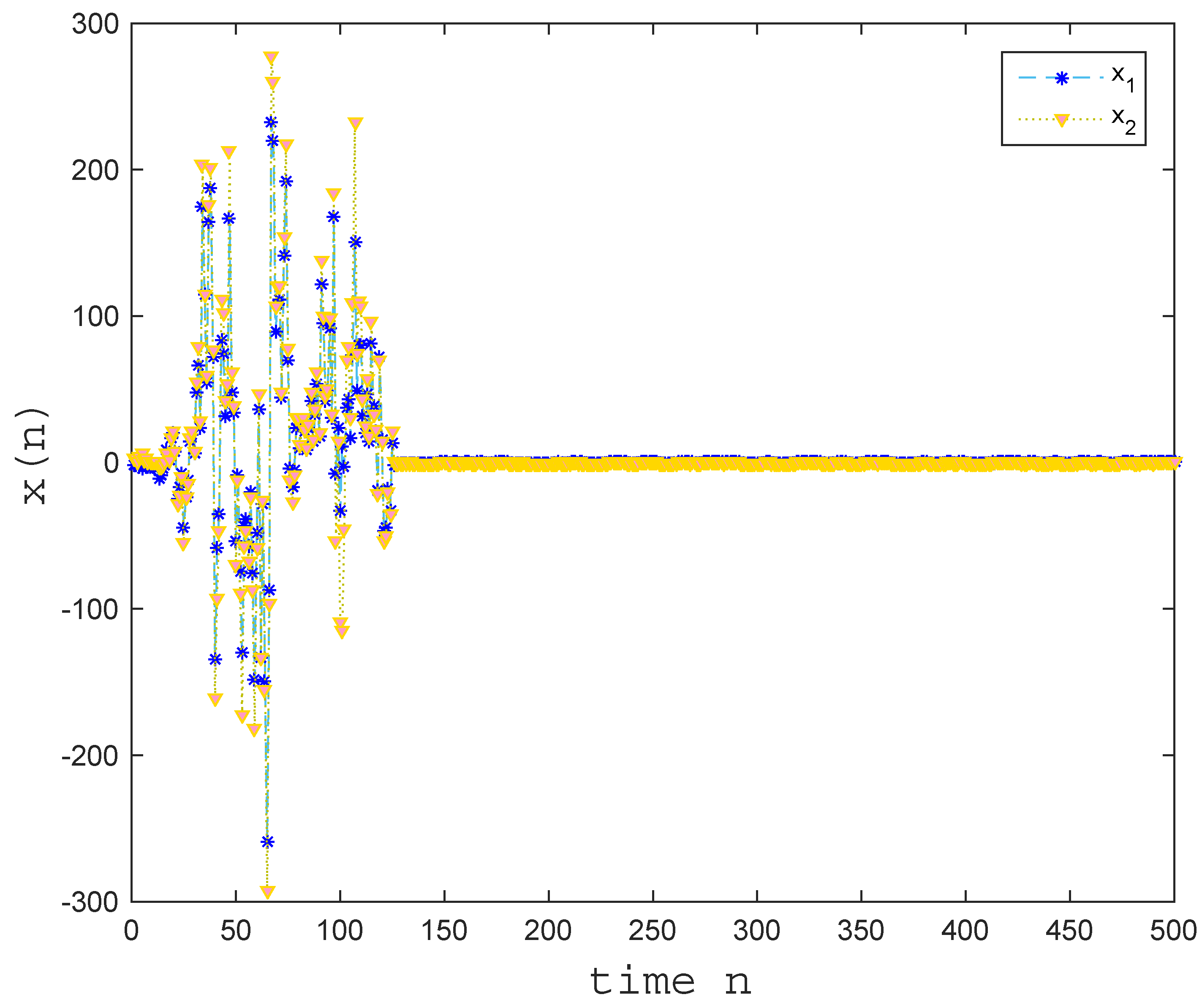
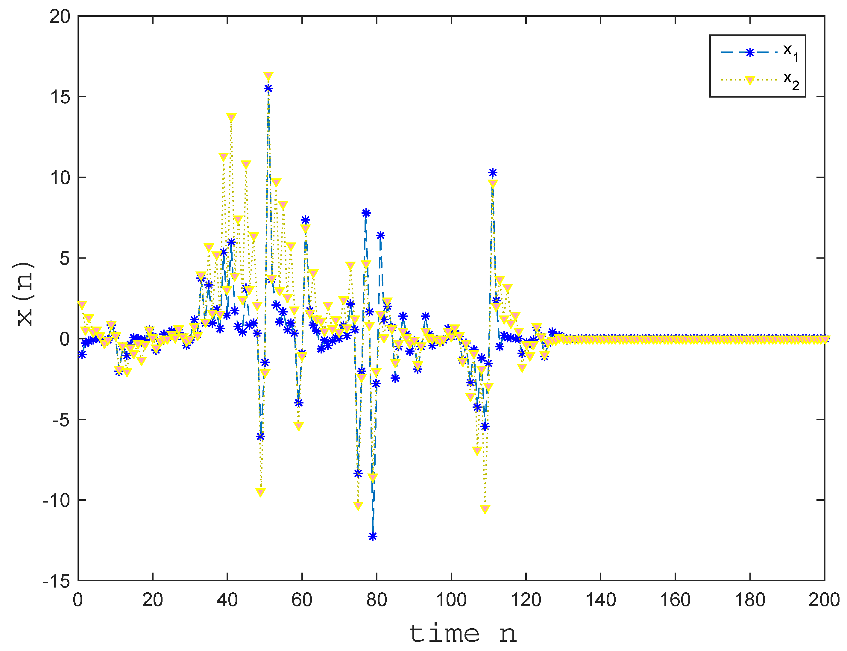
At the end of this section, under an irrestrictive condition, we shall establish a theorem about the almost exponentially stable of system (1).
Theorem 2.
Assume that there exist constants n * 0 , T * 0 and σ > 0 such that conditions (i)–(iii) and the following condition hold:
(iv ) s = n * + k T * n * + ( k + 1 ) T * ( α ( s ) + β ( s ) + ln ρ T a ) σ T * , k N + .
Then the trivial solution of system (1) is pth moment exponentially stable for τ I [ 1 , 1 + log 1 α ^ σ + β ˇ β ˇ q ) .
Proof. 
For convenience, we denote λ ( n ) = α ˇ ( n ) + α ^ 1 τ q β ( n ) + ln ρ T a , α ˇ = sup n N α ˇ ( n ) , and β ˇ = sup n N β ˇ ( n ) .
From the proof of Theorem 1, we conclude that conditions (i)–(iii) guarantee (25) holds, which means that
E | x ( n ) | p c ¯ ξ G b p e s = n 0 n λ ( s ) , n N .
When n I [ n 0 , n * ] , it follows from λ ( n ) α ˇ + α ^ 1 τ q β ˇ + | ln ρ | T a that
s = n 0 n λ ( s ) s = n 0 n ( α ˇ + α ^ 1 τ q β ˇ + | ln ρ | T a ) ( α ˇ + α ^ 1 τ q β ˇ + | ln ρ | T a ) n * ,
which together with (26), implies that
E | x ( n ) | p c ¯ ξ G b p e ( α ˇ + α ^ 1 τ q β ˇ + | ln ρ | T a ) n * , n I [ n 0 , n * ] .
When n I ( n * , + ) , there exist a constant k 0 N such that
n * + k 0 N * n < n * + ( k 0 + 1 ) N * .
Hence, we get that
s = n 0 n λ ( s ) = s = n 0 n * λ ( s ) + k = n 0 k 0 1 s = n * + k N * n * + ( k + 1 ) N * λ ( s ) + s = n * + ( k 0 + 1 ) N * n λ ( s ) = I 0 + k = n 0 k 0 1 I k + I k 0 .
It is easy to calculate that
I 0 = s = n 0 n * λ ( s ) ( α ˇ + α ^ 1 τ q β ˇ + | ln ρ | T a ) n *
and
I k 0 s = n * + ( k 0 + 1 ) N * n ( α ˇ + α ^ 1 τ q β ˇ + | ln ρ | T a ) s = n * + ( k 0 + 1 ) N * n * + ( k 0 + 1 ) N * ( α ˇ + α ^ 1 τ q β ˇ + | ln ρ | T a ) = ( α ˇ + α ^ 1 τ q β ˇ + | ln ρ | T a ) N * .
It is worth noting that
λ ( n ) = α ( n ) + β ( n ) + ln ρ T a + ( α ^ 1 τ q 1 ) β ( n ) ,
which further leads to
I k = s = n * + k N * n * + ( k + 1 ) N * ( α ( s ) + β ( s ) + ln ρ T a ) + s = n * + k N * n * + ( k + 1 ) N * ( α ^ 1 τ q 1 ) β ( n ) ( σ + α ^ 1 τ q β ˇ β ˇ ) N * ,
for k = n 0 , 1 , , k 0 1 .
Form (28)–(32), it can seen that
s = n 0 n λ ( s ) ( α ˇ + α ^ 1 τ q β ˇ + | ln ρ | T a ) ( n * + N * ) + ( σ + α ^ 1 τ q β ˇ β ˇ ) N * k 0 .
Recalling that n I [ n * + k 0 N * , n * + ( k 0 + 1 ) N * ) and τ I [ 1 , 1 + log 1 α ^ σ + β ˇ β ˇ q ) , one gets n n * N * < N * k 0 and σ + α ^ 1 τ q β ˇ β ˇ < 0 , which together with (33), means that
s = n 0 n λ ( s ) ( α ˇ + α ^ 1 τ q β ˇ + | ln ρ | T a ) ( n * + N * ) + ( σ + α ^ 1 τ q β ˇ β ˇ ) ( n n * N * ) = ( σ + α ˇ + β ˇ + α ^ 1 τ q β ˇ ) ( n * + N * ) + ( σ + α ^ 1 τ q β ˇ β ˇ ) n .
By substituting (34) into (26), we have
E | x ( n ) | p c ¯ ξ G b p e ( σ + α ˇ + β ˇ + α ^ 1 τ q β ˇ ) ( n * + N * ) · e ( σ + α ^ 1 τ q β ˇ β ˇ ) n , n I [ n * , ) .
Denote
C = c ¯ max e ( σ + α ˇ + β ˇ + | ln ρ | T a ) n * , e ( σ + α ˇ + β ˇ + α ^ 1 τ q β ˇ ) ( n * + N * ) .
Then, it follows form (27) and (35) that
E | x ( n ) | p C ξ G b p e ( σ + α ^ 1 τ q β ˇ β ˇ ) n , n N .
The proof is complete. □
Remark 4.
In [22], Dai and Xu have investigated the exponentially stable for discrete-time delayed systems by using Razumikhin-type method. However, Theorem 2 proposed in this paper removes this restriction and is applicable to discrete-time delayed systems with impulsive control including both ρ 1 and ρ < 1 , which makes it suitable for a broader scope of applications than the results in [22].
Consider the special case with α ( n ) α and β ( n ) β , here α and β are constants. Similar to proof of Theorem 2, we can obtain the following results.
Corollary 1.
Assume that there exists a non-negative function V ( n , x ) , and exist real constants p > 0 , c 1 > 0 , c 2 > 0 , α R , β 0 , ρ > 0 and σ > 0 , such that
(i) for any x R d and n N , c 1 | x | p V ( n , x ) c 2 | x | p ;
(ii) for any n n k 1 , k N + , E V ( n + 1 , x ( n + 1 ) ) α E V ( n , x ( n ) ) + β sup s N m E V ( n + s , x ( n + s ) ) ;
(iii) for any x R d , k N + , E V ( n k , I ( x ) ) ρ E V ( n k 1 , x ) ;
(iv) α + β + ln ρ T a σ .
Then the trivial solution of system (1) is pth moment exponentially stable.

4. Examples

In this section, two examples to illustrate the effectiveness of the obtained results.
Example 1.
Consider the following discrete-time impulsive stochastic delay system
x ( n ) = f ( n 1 , x ( n 1 ) ) + g ( n τ ( n ) , x ( n τ ( n ) ) ω ( n ) , n n k , n N , x ( n k ) = I k ( n k 1 , x ( n k 1 ) ) , k N +
where ω ( n ) obeys Gaussian distribution N ( 0 , 1 ) . f ( n , x ( n ) ) = e 1 2 sin 2 ( n 1 ) 1 x ( n 1 ) , g ( n τ ( n ) , x ( n τ ( n ) ) = cos n 2 ( 1 + n 2 ) x ( n τ ( n ) ) and τ ( n ) = τ | cos n | + 2 , τ N + . The impulsive perturbation I k ( n k 1 , x ( n k 1 ) ) = e 1 2 x ( n k 1 ) and choosing an impulsive sequence show in (2) for N 0 = 0 and T a = 3 , then the impulsive moments is ζ = { n k | n k = n k 1 + 3 , n 0 = 0 , k N + } .
Let V ( n ) = | x ( n ) | 2 , then
E V ( n ) = e sin 2 ( n 1 ) 1 E V ( n 1 ) + cos 2 n 2 ( 1 + n 2 ) E V ( n τ ( n ) ) ,
which implies that
E V ( n ) e sin 2 ( n 1 ) 1 E V ( n 1 ) + cos 2 n 2 ( 1 + n 2 ) sup θ I [ τ 2 , 1 ] E V ( n + θ ) , n N .
So that condition (ii) of Theorem 2 holds by choosing α ( n ) = e sin 2 ( n 1 ) 1 and β ( n ) = cos 2 n 2 ( 1 + n 2 ) with α ^ = e 1 , β ˇ = 1 2 .
Meanwhile, when n = n k , we derive that
E V ( n k ) = E | e 1 2 x ( n k 1 ) | 2 = e E V ( n k 1 ) ,
which implies that condition (iii) of Theorem 2 holds with ρ = e . Obviously, we conclude that q = min { 1 , e } = 1 . By choosing n * = 0 and T * = 4 π , we derive that
s = 4 k T * 4 ( k + 1 ) T * { ln ( α ( s ) + β ( s ) ) + ln ρ T a } 0.6 π , k N
holds, which implies that condition (iv ) of Theorem 2 is satisfied with σ = 0.15 .
According to Theorem 2, the trivial solution of (37) is exponentially stable in mean square, the state sample trajectory with τ I [ 1 , 1 + 0.7 e ) , initial value ξ = [ 2 , 3.05 ] T are simulated in Figure 1. Figure 1 shows that a system can retain its original stability property with some impulse perturbations that are destabilizing.
Remark 5.
Since the Razumikhin-type method is more conservative than the Lyapunov function method, the Razumikhin-type theorem in [26] is also not convenient to be applied to this system since it is not easy to find an appropriate constant to satisfy the Razumikhin-type condition.
Remark 6.
Since the system without impulses is exponentially stable and the impulses are destabilizing, the existing results in [35,36] cannot be applied to system (37). From Theorem 1 in this paper, we see that the coefficients α ( n ) , β ( n ) have wider range.
Example 2.
Consider the following discrete-time stochastic delay system
x ( n ) = f ( n 1 , x ( n 1 ) ) + g ( n τ ( n ) , x ( n τ ( n ) ) ω ( n ) , n N ,
where ω ( n ) obeys Gaussian distribution N ( 0 , 1 ) . f ( n , x ( n ) ) = e 1 2 ( sin n 1 ) x ( n 1 ) , g ( n τ ( n ) , x ( n τ ( n ) ) = cos n 1 + n 2 x ( n τ ( n ) ) and τ ( n ) = cos 2 n + τ , τ N + .
Proof. 
Define V ( n ) = | x ( n ) | 2 , it can be computed that
E V ( n ) = e sin ( n 1 ) 1 E V ( n 1 ) + cos 2 n 1 + n 2 E V ( n τ ( n ) ) ,
which implies
E V ( n ) e sin ( n 1 ) 1 E V ( n 1 ) , n N .
Similar to the proof of Theorem 1, we can prove that
E | x ( n ) | 2 E | x ( 0 ) | 2 e s = 0 n ( sin ( s 1 ) 1 ) , n N .
Thus, when n + , we have E | x ( n ) | 2 + , which implies that the trivial solution of (40) is exponentially unstable. The simulation results of system (40) with initial value ξ = [ 1 , 2.15 ] T are displayed in Figure 2. □
On the other hand, choose an appropriate impulsive sequence to stabilize the system (40). Setting ζ = { n k | n k = n k 1 + 2 , n 0 = 0 , k N + } , we can derive from systems (40) that
x ( n k ) = e 1 x ( n k 1 ) .
In this case, the average impulsive interval satisfies T a = 2 with the elasticity number N 0 = 0 .
By (41), it can be deduced that
E V ( n ) e sin ( n 1 ) 1 E V ( n 1 ) + cos 2 n 1 + n 2 sup θ I [ τ , 1 ] E V ( n + θ ) .
Thus, it is easy to check that condition (ii) in Theorem 2 holds with α ( n ) = e ( sin ( n 1 ) 1 ) and β ( n ) = cos 2 n 1 + n 2 . Furthermore, we have α ^ = e 2 , β ˇ = 1 .
One can derive from systems (40) that
E V ( n k ) = E | e 1 x ( n k 1 ) | 2 = e 2 E V ( n k 1 ) ,
which implies that condition (iii) of Theorem 2 holds with ρ = e 2 and q = min { e 2 , 1 } = e 2 . Selecting n * = 0 and T * = 2 π , such that
s = 2 k T * 2 ( k + 1 ) T * { ln ( α ( s ) + β ( s ) ) + ln ρ T a } 1.06 π
holds for any k N , which implies that condition (iv ) of Theorem 2 is satisfied with σ = 0.53 and τ I [ 1 , 2.31 ) .
By Theorem 2, we know that system (40) with impulsive control is exponentially stabilized in the mean square. The state sample trajectories are simulated in Figure 3. Figure 3 illustrates that under the stabilizing impulsive effects, all state trajectories of system (40) are forced to approach the trivial solution with an exponential decay rate.
Remark 7.
In Example 2, the impulses are used to stabilize an unstable system. In this case, the impulses must be frequent enough, and their amplitude must be suitably related to the growth rate of the continuous flow.

5. Conclusions

This paper has studied the stability analysis of discrete-time stochastic delay systems with impulses. The stability analysis is achieved with the help of the sums average value of the time-varying coefficients and the average impulsive interval. Some examples were also presented to illustrate the efficiency of the obtained results.

Author Contributions

T.C., Writing-original draft; P.C., Writing-review & editing. All authors have read and agreed to the published version of the manuscript.

Funding

This work was supported by the National Natural Science Foundation of China (No.11771001).

Conflicts of Interest

The authors declare no conflict of interest.

References

  1. Bainov, D.; Simeonov, P. Systems with Impulse Effect: Stability, Theory, and Applications; Ellis Horwood: Chichester, UK, 1989. [Google Scholar]
  2. Lakshmikantham, V.; Bainov, D.; Simeonov, P. Theory of Impulsive Differential Equations; World Scientific: Singapore, 1989. [Google Scholar]
  3. Haddad, W.M.; Chellaboina, V.; Nersesov, S.G. Impulsive and Hybrid Dynamical Systems: Stability, Dissipativity, and Control, Princeton Series in Applied Mathematics; Princeton University Press: Princeton, NJ, USA, 2006. [Google Scholar]
  4. Mao, X.R. Stochastic Differential Equations and Applications; Horwood Publishing Limited: Oxford, UK, 1997. [Google Scholar]
  5. Li, X.D.; Zhu, Q.X.; Donal, O. pth Moment exponential stability of impulsive stochastic functional differential equations and application to control problems of NNs. J. Frankl. Inst. 2014, 351, 4435–4456. [Google Scholar] [CrossRef]
  6. Peng, S.G.; Jia, B.G. Some criteria on pth moment stability of impulsive stochastic functional differential equations. Stat. Probab. Lett. 2010, 80, 1085–1092. [Google Scholar] [CrossRef]
  7. Cheng, P.; Deng, F.Q.; Yao, F.Q. Exponential stability analysis of impulsive stochastic functional differential systems with delayed impulses. Commun. Nonlinear Sci. Numer. Simul. 2014, 19, 2104–2114. [Google Scholar] [CrossRef]
  8. Li, X.D.; Song, S.J. Stabilization of delay systems: Delay-dependent impulsive control. IEEE Trans. Autom. Control. 2017, 62, 406–411. [Google Scholar] [CrossRef]
  9. Li, B. Stability of stochastic functional differential equations with impulses by an average approach. Nonlinear Anal. Hybrid Syst. 2018, 29, 221–233. [Google Scholar] [CrossRef]
  10. Liu, J.; Liu, X.Z.; Xie, W.C. Impulsive stabilization of stochastic functional differential equations. Appl. Math. Lett. 2011, 24, 264–269. [Google Scholar] [CrossRef] [Green Version]
  11. Fu, X.Z.; Zhu, Q.X.; Guo, Y.X. Stabilization of stochastic functional differential systems with delayed impulses. Appl. Math. Comput. 2019, 346, 776–789. [Google Scholar] [CrossRef]
  12. Cao, W.P.; Zhu, Q.X. Razumikhin-type theorem for pth exponential stability of impulsive stochastic functional differential equations based on vector Lyapunov function. Nonlinear Anal. Hybrid Syst. 2021. [Google Scholar] [CrossRef]
  13. Liu, B. Stability of solutions for stochastic impulsive systems via comparison approach. IEEE Trans. Automat. Control. 2008, 53, 2128–2133. [Google Scholar] [CrossRef]
  14. Cheng, P.; Deng, F.Q. Global exponential stability of impulsive stochastic functional differential systems. Stat. Probab. Lett. 2010, 80, 1854–1862. [Google Scholar] [CrossRef]
  15. Wang, Y.H.; Li, X.D. Impulsive observer and impulsive control for time-delay systems. J. Frankl. Inst. 2020, 357, 8529–8542. [Google Scholar] [CrossRef]
  16. Pan, L.J.; Cao, J.D. Exponential stability of impulsive stochastic functional differential equations. J. Math. Anal. Appl. 2011, 382, 672–685. [Google Scholar] [CrossRef] [Green Version]
  17. Chen, G.L.; Gaans, O.V.; Lunel, S.V. Existence and exponential stability of a class of impulsive neutral stochastic partial differential equations with delays and Poisson jumps. Stat. Probab. Lett. 2018, 141, 7–18. [Google Scholar] [CrossRef]
  18. Zhou, B.; Zhao, T.R. On asymptotic stability of discrete-time linear time-varying systems. IEEE Trans. Autom. Control. 2017, 62, 4274–4281. [Google Scholar] [CrossRef]
  19. Zhou, B. On asymptotic stability of linear time-varying systems. Automatica 2016, 68, 266–276. [Google Scholar] [CrossRef]
  20. Zhang, Y. Global exponential stability of delay difference equations with delayed impulses. Math. Comput. Simul. 2017, 132, 183–194. [Google Scholar] [CrossRef]
  21. Zong, X.F.; Lei, D.C.; Wu, F.X. Discrete Razumikhin-type stability theorems for stochastic discrete-time delay systems. J. Frankl. Inst. 2018, 355, 8245–8265. [Google Scholar] [CrossRef]
  22. Zhang, Y.; Sun, J.T.; Gang, F. Impulsive control of discrete systems with time delay. IEEE Trans. Autom. Control. 2009, 54, 830–834. [Google Scholar] [CrossRef]
  23. Dai, Z.L.; Xu, L.G.; Shu, Z.; Sam, G. Attracting sets of discrete-time Markovian jump delay systems with stochastic disturbances via impulsive control. J. Frankl. Inst. 2020, 357, 9781–9810. [Google Scholar] [CrossRef]
  24. Liu, B.; Hill, D.J.; Sun, Z.J. Input-to-state exponents and related ISS for delayed discrete-time systems with application to impulsive effects. Int. J. Robust Nonlinear Control. 2018, 28, 640–660. [Google Scholar] [CrossRef]
  25. Pan, S.T.; Sun, J.T.; Zhao, S.W. Stabilization of discrete-time Markovian jump linear systems via time-delayed and impulsive controllers. Automatica 2008, 44, 2954–2958. [Google Scholar] [CrossRef]
  26. Cai, T.; Cheng, P. Exponential stability theorems for discrete-time impulsive stochastic systems with delayed impulses. J. Frankl. Inst. 2020, 357, 1253–1279. [Google Scholar] [CrossRef]
  27. Wang, P.F.; Wang, W.Y.; Su, H.; Feng, J.Q. Stability of stochastic discrete-time piecewise homogeneous Markov jump systems with time delay and impulsive effects. Nonlinear Anal. Hybrid Syst. 2020. [Google Scholar] [CrossRef]
  28. Ning, Z.P.; Zhang, L.X.; Ali, M.P.C. Stability analysis and stabilization of discrete-time non-homogeneous semi-Markov jump linear systems: A polytopic approach. Automatia 2020. [Google Scholar] [CrossRef]
  29. Dong, Y.L.; Wang, H.M. Robust output feedback stabilization for uncertain discrete-time stochastic neural networks with time-varying delay. Neural Process. Lett. 2020, 51, 83–103. [Google Scholar] [CrossRef]
  30. Niu, B.; Karimi, H.R.; Wang, H.; Liu, Y. Adaptive output-feedback controller dasign for switched nonlinear stochastic systems with a modified average dwell-time method. IEEE Trans. Syst. Man Cybern. Syst. 2017, 47, 1371–1382. [Google Scholar] [CrossRef]
  31. Peng, S.P.; Deng, F.Q.; Zhang, Y. A unified Razumikhin-type criterion on input-to-state stability of time-varying impulsive delayed systems. Syst. Control Lett. 2018, 116, 20–26. [Google Scholar] [CrossRef]
  32. Hespanha, J.P.; Liberzon, D.; Teel, A.R. Lypunov conditions for input-to-state stability of impulsive systems. Automatica 2008, 44, 857–869. [Google Scholar] [CrossRef] [Green Version]
  33. Lu, J.; Ho, D.W.C.; Cao, J. A unified synchronization criterion for impulsive dynamical networks. Automatica 2010, 46, 1215–1221. [Google Scholar] [CrossRef]
  34. Li, X.D.; Li, P. Stability of time-delay systems with impulsive control involving stabilizing delays. Automatica 2021. [Google Scholar] [CrossRef]
  35. Zhang, Y. Exponential stability of impulsive discrete systems with time delays. Appl. Math. Lett. 2012, 25, 2290–2297. [Google Scholar] [CrossRef] [Green Version]
  36. Wu, F.K.; Mao, X.R.; Kloeden, P.E. Discrete Razumikhin-type technique and stability of the Euler-Maruyama method to stochastic functional differential equations. Discret. Contin. Dyn. Syst. 2013, 33, 885–903. [Google Scholar] [CrossRef] [Green Version]
Figure 1. State trajectories of system (37) under destabilizing impulsive perturbation.
Mathematics 09 00418 g001
Figure 2. State trajectories of system (40) without impulsive.
Mathematics 09 00418 g002
Figure 3. State trajectories of system (40) with impulsive.
Mathematics 09 00418 g003
Publisher’s Note: MDPI stays neutral with regard to jurisdictional claims in published maps and institutional affiliations.

