Wavelet Energy Accumulation Method Applied on the Rio Papaloapan Bridge for Damage Identification

Abstract

Large civil structures such as bridges must be permanently monitored to ensure integrity and avoid collapses due to damage resulting in devastating human fatalities and economic losses. In this article, a wavelet-based method called the Wavelet Energy Accumulation Method (WEAM) is developed in order to detect, locate and quantify damage in vehicular bridges. The WEAM consists of measuring the vibration signals on different points along the bridge while a vehicle crosses it, then those signals and the corresponding ones of the healthy bridge are subtracted and the Continuous Wavelet Transform (CWT) is applied on both, the healthy and the subtracted signals, to obtain the corresponding diagrams, which provide a clue about where the damage is located; then, the border effects must be eliminated. Finally, the Wavelet Energy (WE) is obtained by calculating the area under the curve along the selected range of scale for each point of the bridge deck. The energy of a healthy bridge is low and flat, whereas for a damaged bridge there is a WE accumulation at the damage location. The Rio Papaloapan Bridge (RPB) is considered for this research and the results obtained numerically and experimentally are very promissory to apply this method and avoid accidents.

1. Introduction

The structural evaluation to determine damage, deterioration and/or abnormal operating conditions in complex civil structures is essential to determine the operational reliability and residual life of them [1]. Traditionally, most of the damage detection programs are based on visual inspections, which are expensive and limited in access to all parts of the structure. Additionally, the internal damage is not detectable with a visual inspection and it is not possible to obtain a quantitative estimation of the damage or the remaining structural capacity. Recent health monitoring systems for structures include different non-destructive tests, but in all cases the evaluation is localized and do not allow global evaluations of the structures [2].

So far, it has been recognized that vibration analysis and modal analysis are the only techniques that have the potential for global evaluation of structures [1,3]. In these cases, health monitoring is carried out by analyzing changes in the characteristic behavior of vibration through natural frequencies, damping ratios and modal shapes. Many algorithms have been developed to make such a comparison, but, in general, they are classified considering four different approaches: matrix optimization, sensitivity methods, techniques for assigning characteristic values, and minimum range disturbance methods [4]. However, for the particular case of the vehicular bridges it is still necessary to increase the efforts to provide more sophisticated and reliable methods for early damage identification, since there are many documented cases of catastrophic failures of these structures even in the most developed countries.

Two of the most recent and disastrous accidents due to vehicular bridges collapse are related with the Bridge 9340 in the United States of America in 2007 and the Morandi Bridge in Italy in 2018. The Bridge 9340 failed on 1 August 2007, collapsing into the Mississippi River in Minneapolis, Minnesota, USA during the evening rush hour. Thirteen people died and 145 were injured. The bridge transported 140,000 vehicles daily and after the collapse the government recommended the inspection of 700 bridges of similar construction in the country, since after the collapse a possible design defect was discovered on the bridge related to large steel sheets called gusset plates, which were used to connect girders together in the truss structure [5]. On the other hand, the other tragic example occurred on 14 August 2018. During a heavy storm, a 210 m section of the Morandi Bridge in Genoa, Italy collapsed, being one of the most serious collapses of bridges in Europe. As a result of the collapse, three trucks and 35 vehicles fell down from 45 m height to a mountain of rubble. Most of the vehicles and the structure fell into the Polcevera River, others collapsed on the warehouses of an electricity company and on the railway tracks. Around 43 people died according to authorities [6]. Thus, considering that many vehicular bridges around the world could have mistakes within their civil design, wrong selection of materials and even more, which could be operating beyond their useful life and/or overloaded, the probability of structural damage increases and the risk of collapsing, with the corresponding human fatalities and economic losses for not detecting a damage early enough, is high.

The use of vibration signals from the bridges are still considered the most promissory way to detect non-visible damage in this kind of civil structure in a global and online mode; however, those signals have to be post-processed in such a way that damage detection methods could be developed and implemented on the bridges with a low quantity of false alarms and ensuring the reliability of the use of them. The quantity and importance of vibration methods based on wavelets for damage detection on bridges have significantly increased in the last decade, for example, Golmohamadi et al. [7] used a wavelet-based technique to evaluate damage on bridges by using the energy of wavelet coefficients. For this, they used Continuous Wavelet Transform (CWT) in cases of numerical models of healthy and damaged bridges; subsequently they calculated the total energy of the wavelet coefficients as an index of sensitivity to damage. Likewise, McGetrick and Kim [8] investigated the feasibility of a low-cost alternative method based on wavelets for periodic monitoring of bridges, consisting of the use of an instrumented vehicle with accelerometers in their axes. They found that damage can be located more accurately for low vehicle speeds and long bridges, indicating the level of damage by the maximum Wavelet Transform (WT) coefficient from Morlet-type mother wavelets. On the other hand, there are works developed by Reddy and Swarnamani [9] and Walia et al. [10] focused on analyzing the sensitivity of wavelet coefficients to detect and quantify damage on structures. Recently, Quiñones and Montejo [11] evaluated two techniques based on wavelets to identify damage in civil structures. The first technique was based on analyzing the evolution of the structure frequencies through CWT, whereas with the second one they analyzed the singularities generated in high frequencies of the structure response through functions obtained with FWT (Fast Wavelet Transform). The conclusion of the study was that the wavelet parameters should be chosen according to the expected frequency content of the structure and carry out both analyses to ensure efficiency in the damage detection. Zhu and Sun [12] developed a new bridge damage detection index based on Wavelet Energy (WE) change. Their numerical results, using a simply supported beam model, show that with this index it is possible to detect and locate the damage in the structure in a valid way. However, in their simulations they only apply constant excitation and, in reality, the damage could be masked by the effect of environmental excitation, experimental noise and other uncertainties. Those drawbacks faced by Zhu and Sun were addressed in the research carried out by Li and Li [13], whom proposed an index based on the virtual impulse response and WT, named Energy Spectrum Anomaly Measure (ESAM), to identify the existence of damage in civil structures. This research was based on a numerical model of three Degrees of Freedom (DOFs) and they demonstrated that their index is sensitive and reliable to identify damage even in noise conditions. Chen and Oyadiji [14] presented a novel multiple mode wavelet index by using the DWT (Discrete Wavelet Transform) of the modal frequency curves to identify structural damage. With FEM (Finite Element Method)-based models and laboratory tests they demonstrated the functionality of the proposed method. The results suggest that the developed index provides an unequivocal identification of damage compared to the poor resolution offered by the typical WT diagrams to detect damage in the high frequency region when there are high frequency components. Finally, Ercolani et al. [15] showed the implementation of the CWT to detect damage in a FEM model of a bridge with a prestressed concrete slab. They included different types of damage in the structural model, obtained the vertical displacements of the structure under the action of static charges and demonstrated the usefulness of the WT for the detection of damages. Likewise, other recent studies which have had a significant contribution in the topic of damage detection on beams/bridges by using wavelet-based methods can be found in [16,17,18,19,20,21,22,23,24,25,26,27,28].

There are many deteriorated bridges around the world, without an adequate maintenance and without knowing if they have any kind of damage that may lead to their collapse. Additionally, taking into account that an important percentage of the bridges have been operating for decades in seismic regions, with hostile environmental conditions, and/or that mistakes may have occurred during the design and/or construction, the probability of collapse increases. Thus, countries need efficient integral monitoring systems of their main bridges to know their structural condition constantly and avoid catastrophic failures, like the ones presented previously, involving human fatalities and big economic losses. This article presents the development and results of the application (in the cable-stayed bridge RPB) of the wavelet-based method called WEAM, which is capable of detecting, locating (with great accuracy) and quantifying different types of damage on vehicular bridges by using just a few sensors and obtaining the WE. The WE is calculated from the CWT diagrams by means of the area under the curve along the selected range of scale for each point of the bridge deck. The energy of a healthy bridge is low and flat, whereas for a damaged bridge there is an accumulation of WE at the location of the damage. The adequate filtering of the signals and selection of the mother wavelet (Savitzky-Golay filter and Mexican hat mother wavelet, respectively, for the cases here studied) are essential for the success of the method, as it was reported in [29]. The WEAM is applied in detail by using a FEM model with reliable results for identifying damage with high accuracy. On the other hand, regardless of the fact that the WEAM requires a controlled test to be applied in real bridges and that the failure of the RPB took place before this method could be applied, the acquired data for the RPB when it is healthy as well as when a cable broke down are analyzed by using the most useful measurements with random traffic and damage detection is possible by calculating the WE. Thus, the WEAM is promissory to be systematically applied on main bridges to avoid accidents like the one that occurred in the RPB.

2. Proposed Methodology

The detailed step-by-step application of the WEAM for damage detection and localization consists of:

1. Instrument the bridge with vibration sensors proportionally distributed along the bridge deck.

2. Obtain the displacement and/or acceleration vibration responses for the undamaged bridge (baseline) and for the current condition of the bridge to be analyzed while a heavy enough vehicle passes, preferably with constant and low speed and under ambient excitations (mainly wind and pedestrians).

3. Apply an adequate filter to eliminate the greatest quantity of noise (for the cases studied in this article, the best results were obtained by using a Savitzky-Golay filter).

4. Subtract the current (probably damaged) signals and the corresponding healthy signals.

5. Obtain the CWT 3-D colored diagrams for the healthy and subtracted signals. A wide range of scale, adequate mother wavelet (Mexican hat mother wavelet was the most useful for the purposes of this research) and convenient color map must be used.

6. Eliminate the border effects by extending the signals on both sides.

7. Once a clue of damage is detected in the CWT 3-D colored diagrams from the subtracted signals, by comparing with the healthy ones, select the most convenient range of scale.

8. Obtain the CWT 3-D colored diagrams for the healthy and subtracted signals without border effects and for the new convenient range of scale (area of interest).

9. Calculate and graph the area under the curve (WE) for each CWT diagram (different measurement positions for healthy and subtracted cases) along the selected range of scale and along the bridge deck (see Section 2.2).

10. Obtain and graph the average WE considering all the measurement positions for the baseline case and current case (subtracted).

11. Compare the average WE for the baseline case and the current case (subtracted). If they are similar, the current case is also healthy; otherwise, if there is a sudden increment of WE, the current case would be damaged and the position of the damage will be determined by the position of the maximum value of the ridge of WE accumulation (corresponding with the position of the vehicle on the bridge).

It should be noted that, once the characterization of the bridge to be studied is done and the effect of all the possible dangerous damages are known with this method, the steps, including the selection of the most convenient filter, range of scale, and mother wavelet, would be eliminated and the diagnosis would be faster. The schematic diagram of the proposed methodology is presented in Figure 1.

2.1. Description of the Rio Papaloapan Bridge and Its Major Failures

The Rio Papaloapan Bridge (RPB) is a cable-stayed bridge located in the state of Veracruz in Mexico. Built in 1994, it has a main span of 203 m and a total length of 407.21 m with 112 cables distributed in 8 semi-harps (see Figure 2 and Figure 3). The numbering of the cables for each semi-harp is from 1 to 14, the number 1 being the shortest one and 14 being the longest one. Due to the dimensions and importance of this bridge, as well as the major failures that have occurred on it, this bridge was selected for the present research.

The upper anchoring system design [30] consists of one steel plate welded to the anchoring elements, which are cylindrical on one side and flat on the welded side (Figure 4). The cylindrical side is threaded to screw the collar that holds the cable in the upper side.

This bridge, until now, has had two major fractures of the anchoring elements. The first occurred in January 2000, which was due to microstructural deficiencies of the steel. Despite the excellent quality of the steel, a deficient casting process resulted in a low toughness brittle material with a microstructure with large grain size (ASTM 2) and a high content of pores and inclusions [31,32]; in this case, defects in the heat affected zone grew due to fatigue until complete fracture [33]. Unfortunately, no Structural Health Monitoring (SHM) system was implemented at the time this accident occurred.

The second failure occurred on 10 June 2015. In this case, it took place in the weld interface between the anchoring element and the steel plate of cable T1S5 (corresponding with cable 1 of the semi-harp 5). Analyses showed that an initial crack grew due to fatigue until it reached a size of almost 65% of the cross-section area. In Figure 5 clearly two different zones can be identified; the first showed oxidation on its surface after failure, which is characteristic of fatigue growth, indicating that it had sufficient time to seep water into the crack. The second corresponded to the final break due to overload, characteristic of a ductile fracture [34].

After the first failure of the bridge, a full-scope SHM system was installed in 2013, which became the first cable-stayed bridge in Mexico with a full scope remote monitoring system. The system design was based on FBG (Fiber Bragg Grating) sensors and it was configured into 3 sub-systems: sensors, local monitoring and photovoltaic.

The sensor sub-system has 24 strain gages, 24 accelerometers, 1 displacement sensor, 8 tilt meters and 5 temperature sensors, all FBG; the local monitoring system includes a FO interrogator, 1 multiplexor and a computer; and the photovoltaic sub-system has 96 solar cells, 36 deep cycle batteries and their controllers. Additionally, the SHM system includes 2 video cameras, one weather station and a seismological station. The SHM system is communicated via satellite to the CMPEI in the Mexican Institute of Transportation.

The sensors were distributed to analyze the dynamics of the bridge deck and of the four towers; thus, the strain gages (which were used for the purpose of this article) are located 10 under each one of the main girders of the bridge deck, and one on the side at the half height of each tower (L1-L12 and R1-R12 in Figure 6a). On top of each one of the four towers, 2 tilt meters and 2 accelerometers are located. The other 16 accelerometers were placed on the middle of cables 4 and 11 of each semi-harp. The measurements obtained with those tilt meters and accelerometers were not used for the purpose of this article; however, their positions can be figured out by analyzing Figure 3 and Figure 6a. Additionally, in Figure 6b two pictures of sensor R2 installed on the bridge are included.

Although the complete SHM system above described was operating on the bridge before the second failure occurred, the damage was not detected. Since the SHM system was implemented, a historical tracking of the values of the typical parameters, such as natural frequencies, modal shapes, deformations, inclinations, cables tension, etc., has been registered in detail. However, none of them had abnormal variations to warn that there was an important element damaged. Therefore, a reliable method for damage identification is here proposed to avoid bridges’ failures.

2.2. Continuous Wavelet Transform (CWT)

Wavelets are very useful for processing the structural vibration data and performing analyses to assess a structure, since this tool provides information that neither the Fast Fourier Transform (FFT) nor the Short Time Fourier Transform (STFT) can display.

The FFT converts a signal from its original domain (time) to a representation in the frequency domain. Transforming a signal from the time domain to the frequency domain, the time information is lost and it is impossible to determine when a particular event took place. On the other hand, the STFT is a sequence of Fourier transforms of a windowed signal. STFT provides the time-localized frequency information for situations in which frequency components of a signal vary over time, whereas the standard Fourier transform provides the frequency information averaged over the entire signal time interval. However, the major disadvantage of the STFT is the fixed width of the sliding window, which limits the resolution in frequency.

A wavelet is a wave-like oscillation with an amplitude that begins at zero, increases, and then decreases back to zero; that is, wavelets are small waves (signals) highly localized in time that descend rapidly to zero after a few oscillations, and have a null average value (like the signals recorded by a heart monitor). Generally, wavelets are intentionally crafted to have specific properties that make them useful for signal processing; as a mathematical tool, wavelets can be used to extract information from many different kinds of data.

Wavelet Transform (WT) is one of the most important techniques in signal processing to build a framework in the identification of modal properties. As a time-frequency analysis tool, WT has the advantages of dealing with non-stationary, transient and non-linear signals.

The Continuous Wavelet Transform (CWT) is one of the most-widely used forms of the WT, which provides a time-frequency representation of a signal by using a variable-size windowing technique simultaneously. The CWT decomposes the signal into a series of small waves or “wavelets”; those wavelets can be real or complex functions and there is a wavelets’ family available. For each application, a certain wavelet may be more appropriate than others, but, in general, to find it, a trial and error process is required. The selected wavelet is called the “mother wavelet” and can be a function of space or time. Thus, the CWT is generated by choosing a single mother wavelet, and then forming a continuous family of wavelets by translating and dilating the mother wavelet; this is used to sequentially assess the similarity between the mother wavelet and a portion of the signal to be analyzed at all times or locations of the signal. Wavelets with finer scales are an indicator of high frequency information of the signal, while wavelets with coarser scales are appropriate to capture low frequency components. As a result, any irregularity or discontinuity in the signals that are not visible easily by visual inspections or conventional methods may exhibit high values of coefficients through CWT [35].

Thus, while the FFT decomposes a signal into infinite length sines and cosines, effectively losing all time-localization information, the CWT is used to construct a time–frequency representation of a signal that offers very good time and frequency localization. The CWT is an excellent tool for mapping the changing properties of non-stationary signals.

In this way, a mother wavelet function is defined as [36]:

$$\psi \left(t\right)\in L^2(ℝ),$$

(1)

which is limited in the time domain. That is, $\psi \left(t\right)$ has values in a certain range and zeros elsewhere. Another property of a mother wavelet is zero-mean; and the other property is that the mother wavelet is normalized. Mathematically, those two latest properties are represented as:

$${{\displaystyle \int }}_{-\infty }^{\infty }\psi \left(t\right)dt=0$$

(2)

$$\parallel \psi \left(t\right){\parallel }^2={{\displaystyle \int }}_{-\infty }^{\infty }\psi \left(t\right){\psi }^{\ast }\left(t\right)dt=1.$$

(3)

As the translation and dilation properties indicate, the mother wavelet can form a basis set denoted by:

$${\left\{{\psi }_{s,u}\left(t\right)=\frac{1}{\sqrt{s}}\psi \left(\frac{t-u}{s}\right)\right\}|}_{u\in ℝ,s\in ℝ+},$$

(4)

where u is the translating parameter, indicating which region is of concern, whereas s is the scaling parameter greater than zero because negative scaling is undefined. The multiresolution property ensures the obtained set $\left\{{\psi }_{s,u}\left(t\right)\right\}$ is orthonormal. Thus, the CWT is the coefficient of the basis ${\psi }_{s,u}\left(t\right)$, that is,

$$Wf\left(s,u\right)=\langle f\left(t\right),{\psi }_{s,u}\rangle$$

(5)

$$Wf\left(s,u\right)={{\displaystyle \int }}_{-\infty }^{\infty }f\left(t\right){\psi }^{\ast }{}_{s,u}\left(t\right)dt$$

(6)

$$Wf\left(s,u\right)={{\displaystyle \int }}_{-\infty }^{\infty }f\left(t\right)\frac{1}{\sqrt{s}}{\psi }^{\ast }\left(\frac{t-u}{s}\right)dt.$$

(7)

Through this transform, it is possible to map a one-dimensional signal $f\left(t\right)$ to a two-dimensional coefficients $Wf\left(s,u\right)$. The two variables can perform the time-frequency analysis. Then, the location of a particular frequency (parameter s) at a certain time instant (parameter u) can be indicated.

If the $f\left(t\right)$ is a $L^2(ℝ)$ function. The inverse CWT is:

$$f\left(t\right)=\frac{1}{C_{\psi }}{{\displaystyle \int }}_0^{\infty }{{\displaystyle \int }}_{-\infty }^{\infty }Wf\left(s,u\right)\frac{1}{\sqrt{s}}\psi \left(\frac{t-u}{s}\right)du\frac{ds}{s^2},$$

(8)

where $C_{\psi }$ is defined as:

$$C_{\psi }={{\displaystyle \int }}_0^{\infty }\frac{{\left|\mathsf{\Psi }\left(\omega \right)\right|}^2}{\omega }d\omega <\infty ,$$

(9)

where $\mathsf{\Psi }\left(\omega \right)$ is the Fourier transform of the mother wavelet $\psi \left(t\right)$. This equation is also called the admissibility condition.

For the particular purpose of his article, all the types of mother wavelets that can be implemented with MATLAB^© were tried and it was found that the Mexican hat mother wavelet was the most useful due to its satisfactory properties. The nickname, “Mexican hat,” is because the shape of the function is like a typical Mexican hat. The function of this type of mother wavelet is:

$$\psi \left(t\right)=\frac{2}{{\pi }^{1/4}\sqrt{3\sigma }}\left(\frac{t^2}{{\sigma }^2}-1\right)\exp \left(-\frac{t^2}{2{\sigma }^2}\right).$$

(10)

Finally, in order to estimate the WE, which is the parameter that indicates if there is a damage and its location by using the WEAM (as described in Section 2), the area under the curve generated by the wavelets coefficients along the selected range of scale must be calculated for each point of the bridge deck (i.e., from L_min to L_max, where L is the total length considered for the bridge deck), as it is represented in the following equation just for one point of L:

$$WE={{\displaystyle \int }}_{s_{min}}^{s_{max}}f\left(Wf\right)ds$$

(11)

where s_min and s_max are the minimum and maximum values of scale, respectively, from the range of scale selected; whereas $f\left(Wf\right)$ represents the function of the curve of the coefficients along the selected range of scale just for one point of the total length (L) considered. In this way, after obtaining the WE for all the points of L, damage can be detected and located, because the corresponding total WE of a healthy bridge is a low and flat curve, whereas for a damaged bridge the corresponding WE curve is higher and there is a WE accumulation at the damage location, as it will be demonstrated in the next section.

3. Validation of Proposed Methodology

In this section, the proposed method explained meticulously in Section 2 is applied for its numerical validation. Thus, for this purpose, a detailed FEM model of the RPB is developed in ANSYS^© in order to study different scenarios of damage included damaged deck and damage on cables (simulating the failure of a cable occurred in 2015 into the real bridge). The numerical transient responses obtained while a constant force (load) moves on different nodes along the bridge deck (simulating a vehicle passing through the bridge) as well as the experimental signals from the real bridge are post-processed with a code written in MATLAB^© (R2017a), which provides the Wavelet Energy (WE) and determines if a damage exists and its location.

The numerical results obtained applying the WEAM show the great capability of this method to detect damage and locate it with high precision, even when significant percentage of noise was included in the signals. On the other hand, regardless that the WEAM is useful with a controlled test and the failure of the RPB took place before this method could be applied, the acquired data from the real bridge when it was healthy as well as when a cable broke down are analyzed by using the most useful measurements and damage detection is possible by calculating the WE. Thus, the WEAM is promissory to be systematic applied on the main bridges to avoid accidents like the one occurred in the RPB in 2015.

3.1. Numerical Simulation

3.1.1. Cable-Stayed Bridge Finite Element Model

A numerical FEM code named “BRITRANSYS” was written in ANSYS^© (V 14.0) and contains two parts: (a) A detailed model based on the characteristics of the RPB with the possibility of including different types of damage like damage on deck and cables; (b) the transient solution/responses obtained while a force moves on different nodes along any section or the whole bridge deck (simulating a vehicle passing through the bridge), different speeds and weights for the “vehicle” can be considered and the dynamic responses (displacements and accelerations) can be obtained in any node of the model.

As for the FEM model, the ANSYS APDL^© code was built as follows: The model geometry of the RPB was created in AutoCAD^©, then became APDL^© commands through an Excel^© sheet in the form of keypoints coordinates; initial/final keypoints were defined for each line. The writing of commands for areas was made by using simple APDL^© commands, mainly “*DO”.

Three different types of elements were used to build the model: BEAM188 for towers, main girders and transverse girders; SHELL181 for slab; and LINK180 for cables. Then the material properties were defined for each structural element as well as the cross-sectional properties.

BEAM188 is a 3-D two-node beam element suitable for analyzing slender to moderately stubby/thick beam structures. The element is based on Timoshenko beam theory which includes shear-deformation effects and it has six or seven DOFs at each node. SHELL181 is a four-node structural element with six DOFs at each node: Translations in the three directions, and rotations about the three axes. It is suitable for analyzing thin to moderately-thick shell structures. LINK180 is a 3-D spar/truss element that is useful in a variety of engineering applications. This element is a uniaxial tension–compression element with three DOFs at each node: Translations in the three nodal directions. Tension-only (cable) and compression-only (gap) options are supported. Plasticity, creep, rotation, large deflection and large strain capabilities are included and no bending of the element is considered.

Every cable in the bridge has specific values of area, mass and stress (related with tension). Stresses data were load to the software in a vector array with 112 spaces, the spaces were filled by loading data with the “*VREAD” command, this command takes the data previously stored in a “.txt” extension file. Then, area and mass values were assigned to each line that correspond to a cable. Previously, for meshing the structural elements, their attributes like cross-sectional area, material and element type were assigned to each different structural elements group. Once this was done, the whole model was meshed to be composed of 7365 elements and 8053 nodes. Finally, the restrictions and the initial state that define the initial stress of every cable were defined. To finish a base bridge model, the command “SOLVE” was set.

Likewise, in order to obtain the displacement/acceleration dynamic responses, a specific lane where the moving load passes and the corresponding longitudinal section of the bridge deck were defined, then the respective nodes one after the other (in straight line shape) were created and consecutively numbered. After that, the moving load simulating a vehicle was defined with a specific weight and speed and set on each node through the ANSYS^© transient solution. Finally, this part of the code defines the nodes and the responses to be obtained, then the corresponding data are saved in “.txt” format to be post-processed. Figure 7 shows the healthy FEM model which was calibrated with experimental results obtained from the RPB monitoring.

On the other hand, a MATLAB^© (R2017a) code called “MAT_BRITRANSYS” was developed in order to post-process the signals from the FEM model/simulations and follow the methodology (WEAM-Wavelet Energy Accumulation Method) for damage detection. This code loads two numerical simulations from the ANSYS^© code (one healthy and one damaged in “.txt” format) for different measurement positions along the considered longitudinal bridge deck section (the same measurement positions for healthy and damaged cases), and provides: time-domain plots (waveforms), frequency-base plots (FFT’s), spectrograms and CWT 3-D colored diagrams; all for original, noisy (Gaussian noise added) and filtered (Savitzky-Golay filter used) signals. Even more, this code also post-processes the CWT diagrams and performs subtractions (damaged signals-healthy signals), removes the border effects (by means of signal extensions) to bring the border effects to “inexistent” parts of the considered bridge deck, calculates the total wavelet energy for all the respective bridge deck for each point of measurement, and makes an average of the total wavelet energy considering the different positions of the measurements. Then, a damage can be detected and its location identified by means of the accumulation of this energy. For analyzing the real data from the RPB, the same code was used with some modifications according to the quantity, position and type of sensors.

3.1.2. Results from Numerical Simulations

Two of the most dangerous faults that can lead to the collapse of the RPB (as in any cable-stayed bridge) are a damage on the deck and a damaged cable. Both cases are studied in this section considering the FEM model and applying the WEAM, as it was described in Section 2.

All the types of mother wavelets that can be selected with MATLAB^© and different types of filters were implemented; the best results to identify damage were obtained with the Mexican hat mother wavelet and a Savitzky-Golay filter.

The first case studied was a damage on the deck, simulated by reducing by 30% the cross-sectional area (0.30 h, where h is the height of the deck) in 5% of the 203 m length bridge (bridge deck between pylons). The cross-section of the deck is rectangular with a height (h) = 0.20 m and a width (w) = 23.40 m. The damage was placed at 25%, 50% and 75% of the considered length of the bridge deck (one at time) and the measurement points were established at 25%, 50% and 75% of the considered length of the bridge deck (all at the same time for each case of healthy bridge and bridge with a single damage). It is important to mention that, under the deck (slab), the bridge has a very rigid structure composed by two main girders and 117 transverse girders; therefore, that reduction of 30% of the cross-sectional area impacts in a stiffness reduction of 22% on the damaged section.

As it has been notified [8,29], low vehicle speeds allow damage identification more accurately on long bridges. However, the selection of a vehicle with low speed crossing all the RPB would impact significantly in computing time. Thus, in the interest of reducing the computing time, a moving force representing a vehicle type T3S3 (nomenclature not related with the corresponding of cables and semi-harps) fully loaded (54,000 kgf) was selected to cross just the bridge deck between pylons; that is, L = 203 m (instead of 407.21 m) with a speed of 1 m/s and sampling frequency of 64 Hz. This configuration and selecting an adequate resolution for the CWT diagrams according to the range of scale allowed having an equilibrium between computing time and accuracy of results for damage identification. It should be noted that it does not matter if the vehicle starts its movement at the first node or later, the results for identifying damage are not affected as long as the vehicle passes at the damage location. The selected lane for the moving force was the right lane of the downstream side and the measurement points were located on the corresponding nodes of the right side of the deck (downstream side) where the moving force does not pass. It is important to notice that regardless the CWT provides pseudo frequency (scale)-time domain info, if the vehicle speed is known (as it happens in the numerical simulations) then the CWT diagrams are easier to analyze by including the length of the bridge deck (distance) instead of time, so that we can know the damage position on the bridge corresponding with the vehicle position.

In Figure 8, the CWT diagrams for a healthy bridge deck and a damaged bridge deck at 25% of L obtained from the corresponding acceleration signals at the three locations are shown. As it can be observed in this figure, for this initial wide range of scale (from 1 to 500) there is a tiny clue of damage around 0.25 L, but it is not very evident because it is partially masked. In this range of scale, the WE is amplified mainly in the zone of the influence of the first natural frequency and secondly in the regions of the border effects (around 0% and 100% of L) and damage (around 25% of L), hindering a clear damage identification. Thus, comparing the damaged diagrams (Figure 8b) with the corresponding ones of the healthy case (Figure 8a) could seem very similar each other; however, the presence of damage is there but masked.

In order to increase the evidence of damage, the signals used for obtaining the diagrams shown in Figure 8 were subtracted (damaged ones—healthy ones) and then the resultant signals were extended by using the MATLAB© command “wextend” (antisymmetric-padding) for eliminating the border effects. In Figure 9, the subtracted and extended CWT diagram is shown just for one measurement in the interest of brevity. It can be observed that the border effects were taken out of the real bridge length considered; whereas the useful subtraction effect cannot be clearly distinguished yet because the scale range is not the convenient. Therefore, just the zone inside the yellow square must be considered, in this way the real bridge length is again analyzed (but now without border effects), whereas the scale from 250 to 500 allows to focus on the damage effect and the influence of the subtraction will be appreciated. Likewise, once the step related with the subtraction of signals was applied, the cases presented in every figure as “damaged bridge” correspond with the use of the subtracted signals.

Thus, the CWT diagrams for the three measurement positions considering the region of the yellow square are shown in Figure 10b and the respective ones for the healthy bridge are shown in Figure 10a. Comparing those figures, the presence of damage is clear with evident indicators of high wavelets’ coefficients (energy) around the damage location. It should be noted that damage identification is possible even if the measurements come far away from the damage position; however, the closer the measurement is to the position of the damage, the greater the energy, as it will be shown next.

The WE energy for a healthy and a damaged bridge deck was calculated for each point of the considered length by means of the area under the curve along the adjusted range of scale. The results for healthy and damaged cases are shown in Figure 11, where it can be observed that the WE for the healthy cases is very low and flat with tiny WE accumulation at the measurement points and at the ends because of the remaining border effects. Whereas, for the damaged cases, no matter the measurement point, the WE accumulation is always around the damage location and its magnitude is much higher compared with the healthy cases. Even for the case of measurement at 0.75 L, the percentage of error for the damage localization is very acceptable (4.1%), while for the other two measurements it is smaller due to the closeness with damage (2.8% and 1.6% for measurement at 0.50 L and 0.25 L, respectively). The advantage of this method of detecting damage using just one point of measurement far away from damage is interesting.

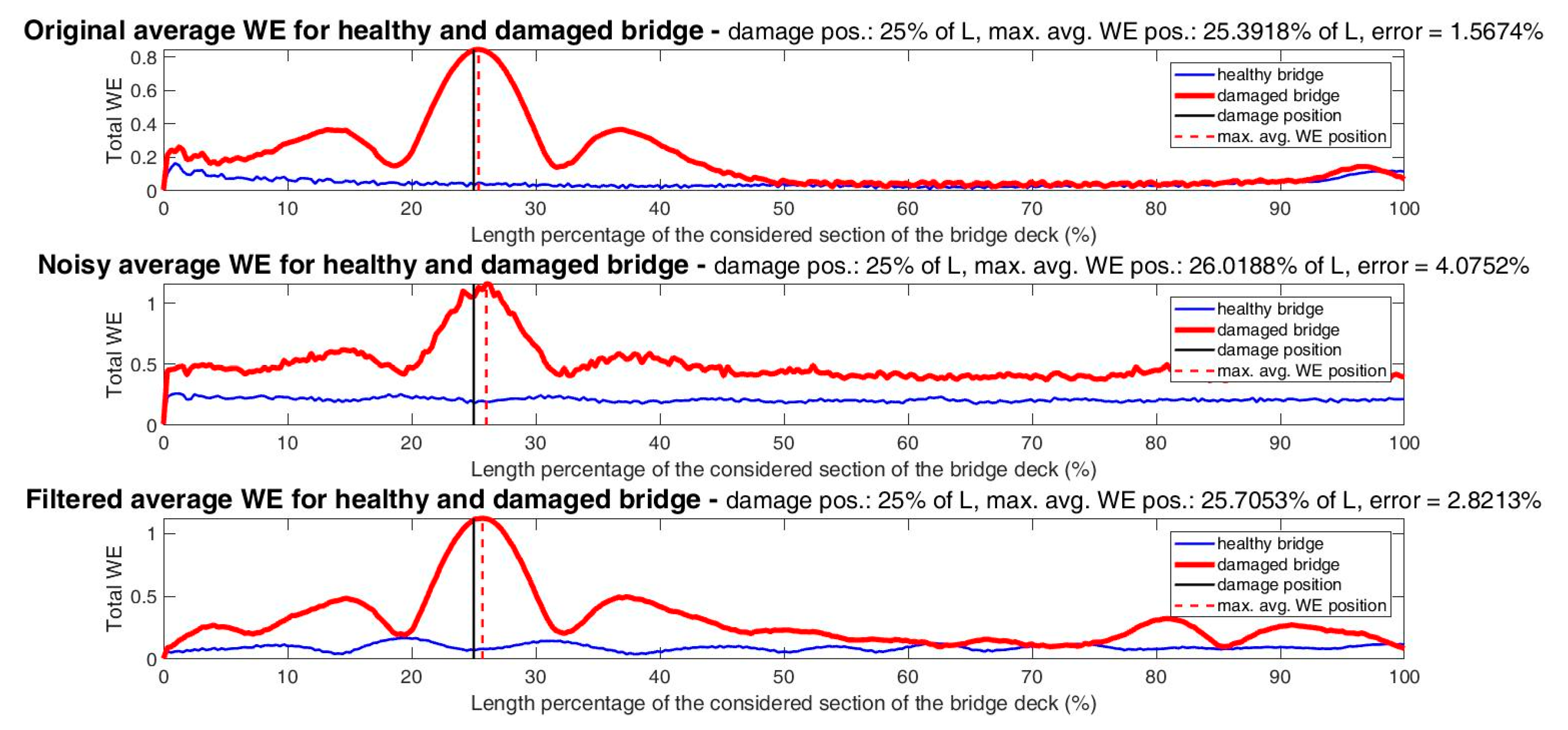
In real cases, just one value of the total WE would be useful and; therefore, the average of the WE considering all the measurement points must be calculated. Moreover, it must be taken into account that the signals would contain significant percentages of noise, making the damage identification difficult and requiring a useful filter. Thus, in Figure 12, the total WE for all the measurement positions and respective averages are presented for healthy and damaged cases considering the original, noisy and filtered signals. The original signals are signals generated with the FEM simulations and no noise was added and no filters were used (like the ones used for the previous diagrams exhibited); for the noisy signals, 15% of Gaussian noise was added; and for the filtered signals a Savitzky-Golay filter (order = 2; window length = 19) was implemented for the noisy signals. It can be observed in Figure 12 that the percentage of error in damage identification for average noisy signal increased 2.6 times with respect to the original case (still acceptable considering the big percentage of noise added). Whereas, for the filtered case, the percentage of error was reduced 1.4 times with respect to the noisy case. In all the scenarios, damage detection and localization were possible and the percentage of error was less than 5.0%.

Lastly, for an easy visualization, in Figure 13 just the average WE is shown for a healthy and a damaged bridge deck and for the three scenarios of signals (original, noisy and filtered), with the respective percentage of error. It is important to notice that if the considered vehicle speed is set to 2, 3, 4 and 5 m/s, the percentage of error for the damage location considering the original signals changes to 1.85%, 2.15%, 2.49% and 2.91%, respectively. Whereas, for the speed of 1 m/s, the corresponding percentage of error is 1.57%, as it can be observed in Figure 13.

Likewise, the damage location was changed and set on the midspan between pylons (0.50 L) and at 0.75 L. The noisy and filtered CWT diagrams for the area of interest are shown in Figure 14 for damage at 0.50 L and in Figure 15 for damage at 0.75 L. Whereas, the total average WE energy from original, noisy and filtered signals are shown in Figure 16 for a healthy and a damaged bridge deck at 0.50 L and in Figure 17 for a healthy and a damaged bridge deck at 0.75 L.

The CWT diagrams shown in Figure 14 and Figure 15 are overwhelming for damage identification at 0.50 L and 0.75 L, respectively. By using the noisy signals, the damage identification is evident because of the change of color representing higher wavelets’ coefficients. Whereas, by using the filtered signals, the CWT diagrams are clearer and the damage identification is even easier.

As for the total average WE, that WE is high for both cases of damaged bridge deck (at 0.50 L and 0.75 L) and low for the healthy corresponding cases (see Figure 16 and Figure 17). Moreover, the WE for the damaged signals is accumulated in the vicinity of the damage position and, in this way, the differences between the positions of the maximum values of the average WE and the values of the respective damage positions are very small, whereas, for the healthy cases, there are no remarkable accumulations.

Taking into account the case of damage at 50% of L (Figure 16), the percentage of error for the damage identification by considering the maximum value of the WE accumulation was 0.31% for the original signal, then it increased three times for the noisy signal and, finally, it came back to the same original absolute value for the filtered signal (0.31%). For the original signal, damage was identified slightly to the right of the real position, whereas, for both the noisy and filtered signals, damage was identified slightly to the left of the real position.

On the other hand, considering the damage at 75% of L (Figure 17), the absolute percentages of error for the damage identification were 0.10%, 0.73% and 0.31% for original, noisy and filtered signals, respectively. For the original signal, the damage was identified slightly to the left of the real position, whereas, for noisy and filtered signals, it was identified slightly to the right of the real position.

Thus, by using the acceleration signals and following sequential steps for consolidating the WEAM, damage was detected and located with high accuracy; no matter its position on the bridge deck, the condition of the signals (original, noisy or filtered), the quantity of the measurement points (single or average of multiple points) nor the location of the measurement points (on the damage, close or far away). It is important to mention that once the area of interest is determined on the CWT diagrams, damage identification becomes easy on the very same CWT diagrams and the total average WE diagrams will confirm the existence and location of damage. Furthermore, those WE diagrams help provide a value of the maximum WE to quantify how severe the damage is.

The same case of damage analyzed above by using the acceleration signals is henceforth studied with the corresponding displacement signals from the vibration of the bridge. In Figure 18 the CWT diagrams from original displacement signals at three different positions are shown for a healthy and a damaged bridge deck at 25% of L. A huge initial scale range was used (from 1 to 10,000) in order to explore a clue of damage and again, at a glance, no clear indications of damage were found.

After performing the signals’ subtractions and extensions, as well as using the useful range of scale (from 250 to 500), the previous diagrams now look like those in Figure 19. In the new figure it is possible to see that there are no border effects. Moreover, the energy for the healthy cases (Figure 19a) is accumulated around the measurement point, as expected, but that energy is low, as it can be observed in Figure 20a.

On the other hand, for the damaged case, all the energy is accumulated around the damaged location no matter the measurement point. Additionally, out of the zone of damage the energy is practically zero, which was achieved by means of the signals’ subtraction, which is why the shape of the energy expansion looks almost identical for all the cases of damage with different measurement positions (Figure 19b). However, the energy is higher as long as the measurement point is closer to damage, as it can be seen in Figure 20b.

Part of the energy accumulated in the zone of damage is lost during the subtraction, but the advantage is that no energy will be displayed in the zone of the measurement when damage is not there and the plots will look clearer. Whereas the disadvantage of lost energy because of the subtraction and the far measurements can be compensated with the average of the WE.

Now, in the interest of brevity, just the filtered displacement signals were used to calculate the total average WE diagrams, because this is the most realistic scenario to deal with. That is, the signals will always contain noise and a filter has to be used to reduce that noise. Thus, in Figure 21, the corresponding total average WE diagrams for healthy and damaged bridge deck at 0.25 L, 0.50 L and 0.75 from filtered displacement signals are shown. In Figure 21 the difference of WE between healthy and damaged cases is evident; therefore, the existence and location of damage was confirmed and the percentage of error was again very low (no more than 1.60%).

In order to quantify the severity of damage and the sensitivity of this method, four different magnitudes of this type of damage on the bridge deck, additionally to the one studied above, were simulated at 25% of L, for a total of five cases, that is: 0.10 h, 0.20 h, 0.30 h, 0.40 h, and 0.50 h of height reduction. The total average WE’s for all these cases are shown in Figure 22. The signals used for those plots were the acceleration signals after being added with 15% of noise and then filtered. This was in order to analyze the most common signals available in real SHM (acceleration) and their condition (noisy and then filtered). The tiny differences of the healthy WE’s for the different diagrams of Figure 22, even when the original healthy signals are obviously the same, are due to the randomness of the added noise. The code was configured to analyze one healthy case and one damaged case at the same time. Consequently, the healthy case was run for each case of damage and the noise was not the same, thus the filtered WE’s were not identical.

Additionally, in Figure 23 it is possible to see the healthy average WE and all the damaged average WE’s together in the same plot, for an easier visualization of the impact of the magnitude of damage in the WE and the sensitivity of this method.

In

Table 1. Analysis of damage severity for different magnitudes of damage on the bridge deck at 0.25 L presented in Figure 22 and Figure 23.

Analysis of Damage Severity on Bridge Deck at 0.25 L
Damage Magnitude	Max. Avg. Damaged WE	Max. Avg. Damaged WE/ Max. Avg. Healthy WE	Error in Damage Localization (%)
0.10 h	0.37	2.22	5.33
0.20 h	0.60	3.55	4.08
0.30 h	1.12	6.65	2.82
0.40 h	2.46	13.32	1.57
0.50 h	7.65	41.35	1.32

, a summary of the results shown in Figure 22 and Figure 23 is presented. In the table, as expected, it is clear the tendency about the increment of damaged WE and ratio of maximum average damaged WE/maximum average healthy WE as the severity of damage increases; as well as the increment of the damage localization accuracy as the magnitude of damage increases. Nevertheless, the highest percentage of error in those cases presented in Table 1 (5.33%) is still very acceptable considering the low magnitude of damage (0.10 h), high percentage of noise (15%) and the kind of signal used (acceleration instead of displacement).

The experimental validation of the quantification of damage will be performed by using a lab model in future works, since in the real bridge is not possible. Cracks of different severity will be induced on the deck of the lab model in order to correlate the different WE curves with the corresponding level of damage.

Finally, in regards to the numerical part of this article, for the other type of damage (damaged cable) just three cases were analyzed: healthy bridge, bridge with damaged cable T1S5, and bridge with damaged cable T10S7. For all those cases, the total length of the bridge had to be considered (407.21 m) and again three points of measurement were established, this time at 0.33 L, 0.50 L and 0.66 L instead of 0.25 L, 0.50 L and 0.75 L. This was because the first point and the last one would have been located practically on the pylons and it was not convenient, then the best distribution to keep just three measurement points was two points at 1 L/3 and 2 L/3 and one additional at the mid-span (1 L/2).

The case of damaged cable T1S5 corresponds with the real case analyzed in the next section, where cable 1 of the semi-harp 5 collapsed and whose failure was described previously. The anchor of this cable on the deck (according to the lateral view of Figure 3 from left to right) is found at 0.77 L, and there was no numerical point of measurement at this location (the nearest one at 0.66 L which represents 42 m of distance). The tension of this cable was reduced by 40%.

As for the damaged cable T10S7, this cable is number 10 of semi-harp 7 and is anchored at 0.42 L (practically between the first and second numerical measurement points with around 32 m of distance) and its tension was reduced by 50%. The purpose of this latest case was to analyze other locations of damaged cable and the magnitude of lost tension.

Since the considered current length of the bridge is twice the previous length taken into account for analyzing damage on the deck, in order to reduce the computing time and avoid a crash up of any of the two codes used with either ANSYS^© or MATLAB^©, the sampling frequency was halved (32 Hz). The moving force represented again a vehicle type T3S3 fully loaded (54,000 kgf); however, now to cross the whole bridge (L = 407.21 m) with a speed of 2 m/s. The selected lane was the right lane of the upstream side and the measurements were established on the nodes of the right side of the deck (upstream side) where the moving force does not pass. Higher vehicle speeds were simulated with excellent results for detecting and locating damage with good accuracy, but just the lowest speeds were included in this article in the interest of brevity.

As it was explained before, by the time the fault of the T1S5 occurred, the instrumentation was not planned for acquiring useful data for being used with this WEAM and, unfortunately, the acceleration sensors were not placed on the deck. Thus, considering the available instrumentation when the cable broke, the strain measurements of the deck would be the most useful ones and; therefore, for these numerical simulations, just the displacement signals were used.

In Figure 24, the original CWT diagrams are shown for the healthy case and bridge with damaged cable at 0.77 L, before and after the signals subtraction, just to show that, even when the convenient range of scale had not been selected yet, the subtraction was very useful to start providing a clue of the damage location. In Figure 25, the original CWT diagrams without border effects and for the area of interest are shown for the three cases (healthy, damaged cable at 0.77 L and damaged cable at 0.42 L), and the perspective to observe the magnitude of the coefficients for the damaged cable T1S5 is shown in Figure 26. Lastly, in Figure 27, the corresponding total filtered average WE’s can be observed.

In Figure 24, small differences between the healthy bridge case and the bridge with damaged cable at 0.77 L before the signals subtraction are observed for the original wide range of scale (1 to 10,000). However, after the signals subtraction, the corresponding CWT diagrams show evident inclinations of the highest coefficients toward the damage location for the same range of scale; this helped to provide a clue of the damage location and define the range of scale to calculate the WE.

The detection and localization of the damaged cables were possible by using the same range of scale defined as the most convenient for damage on the deck (250 to 500). However, in order to use a wider range of scale where the highest coefficients have influence around the damage locations, the convenient range of scale for these cases of damaged cables was defined from 250 to 1500 and the corresponding CWT diagrams for the area of interest are exposed in Figure 25, the evidences of damage are clear. Additionally, in Figure 26 the magnitude of the coefficients around 1000 can be appreciated for the case of damaged cable T1S5, which is useful to compare with the real case and numerical damage on deck.

Finally, in Figure 27, the total filtered average WE for each case of damaged cable compared with the healthy case are presented. For the damaged cable T1S5 (at 0.77 L), the percentage of error in the damage location was 2.20%. On the other hand, the maximum WE of the damaged curve was approximately 2.5 times the maximum WE of the healthy case and the same magnitude higher (2.5), with respect to the second bigger ridge of the same damaged curve. That is, the ridge of maximum WE accumulation indicating the damage location at 0.77 L is high enough to be distinguished to the second highest ridge of the same curve and the first highest ridge of the healthy curve. For the case of damaged cable at 0.42 L, the maximum WE increased 1.6 times with respect to the corresponding value for damaged cable at 0.77 L, which can be due to the more critical position of this cable and greater loss of tension percentage. The percentage of error for its damage location was also very acceptable (4.47%) considering that the signals were added with noise and then filtered.

The significant increments of the WE for the cases presented in Figure 27, in relation to the cases of damaged deck shown previously, are attributed to the damage nature and the consideration of a wider range of scale.

Thus, in this section it was demonstrated that, if the WEAM is applied as it was explained in Section 2, detection and location of different types of damage in a vehicular bridge is possible with high precision and by using just a few sensors. Moreover, this method also allows distinguishing among different severities of damage.

3.2. Results from the Real Failure Case

In this section, the most useful available data acquired during the monitoring of the second major failure of the RPB that occurred on 10 June 2015 (collapse of cable 1 of the semi-harp 5-T1S5) are analyzed and compared with the respective ones of the bridge when it was thought to be healthy (baseline) on 22 August 2014. These data corresponded with the measurements on the deck obtained with strain gages (125 Hz of sampling frequency), see Figure 6a.

As it was mentioned previously, a controlled test, with the adequate instrumentation to follow the steps of the WEAM, was not possible to be performed early enough to warn about the damage on cable T1S5, thus to avoid its fault. Nevertheless, the data acquired with random traffic almost a year before the incident (healthy case), and some minutes before the collapse of the cable (damaged case), are valuable to demonstrate that this method is promissory and its application could have avoided this failure and will avoid accidents in the future.

First, in Figure 28b the filtered damaged spectrogram (based on the STFT) of measurement point R2 (see Figure 6a) is shown for 840 s of monitoring. An evident mark at around 674 s can be distinguished and corresponds with the instant when the cable broke; however, before and after that event, there are no indicators about a damaged cable nor the absence of a cable, even when the signal was filtered and the measurement point is the nearest to the anchor of the damaged cable on the deck. Furthermore, comparing the first 670 s of Figure 28b (when damage existed and failure was imminent) with Figure 28a, which shows the respective spectrogram for 120 s of baseline acquisition, no clue of damage can be established and they look very similar to each other.

On the other hand, the WE was always clearly higher for the damaged measurements instead of the healthy ones. This was observed for all measurement points by analyzing the CWT and WE diagrams for different periods of 120 s of damaged signals acquired on June 10, 2015, before the accident, and periods of 120 s of healthy signals acquired on August 22, 2014, as well as for the few months before and after that latest date. However, in the interest of brevity, just the CWT and WE diagrams from three measurement points (R1, R2 and R4) and for the same 120 s of the spectrogram of Figure 28a are shown for the healthy case and for the first 120 s of the spectrogram of Figure 28b for the damaged case.

Comparing the CWT diagrams of Figure 29 (healthy) and Figure 30 (damaged) without border effects and for the area of interest suggested in the numerical part (scale from 250 to 500), the higher wavelet activity and higher wavelets’ coefficients for the damaged case with respect to the healthy case are evident. Additionally, in Figure 30 it can be seen that the highest wavelets’ coefficients for the damaged case were obtained for the nearest measurement point to the damage (R2). That is, the location of this measurement was the nearest to the anchor of cable T1S5 on the deck. These results had to alert that the bridge was damaged due to the significant increment of the wavelets’ coefficients in relation to the baseline case and had to suggest that damage was located around R2.

As it was mentioned previously, the results of just three measurement points were displayed. However, even considering the rest of the measurements, R2 showed the highest wavelets’ coefficients. Additionally, in order to know how big the increment of wavelets’ coefficients was at the moment of cable T1S5 collapse, the corresponding CWT diagram is shown in Figure 31. Regardless of the fact that multiple factors included in real data cannot be represented numerically, and that the types of signals were not the same, there is a good agreement about the magnitude of the wavelets’ coefficients for numerical and experimental cases of RPB with the damaged cable.

Finally, the total WE’s obtained from the CWT diagrams of Figure 29 and Figure 30 are shown in Figure 32. In Figure 33, the corresponding total average WE for the healthy and damaged cases are exposed into the same plot. The WE’s for single measurements are clearly higher for damaged cases (Figure 32) and the maximum total average WE is almost five times higher for the damaged case with respect to the healthy case (Figure 33). This exercise was additionally made for four different periods of 120 s of the healthy bridge and the damaged cable, and in all the cases the average WE was higher for the damaged bridge and the magnitudes of the maximum average WE’s were similar to the ones shown in Figure 33. Then, regardless of the randomness of the traffic, significantly higher WE was observed for the damaged bridge and the detection and localization of the damage was possible. Nevertheless, in future works a controlled test will be performed during the maintenance programs, which involves the removal of cables for changing damaged upper anchoring systems, and, in this way, each step of the proposed method will be carried out for a precise validation.

Considering the exhaustive and interesting review of bridge monitoring using passing vehicles presented in [37], with a summary table of the most promissory methods for damage detection, the method here proposed has the advantages of detecting, locating (with great accuracy) and quantifying different types of damage on vehicular bridges by using just a few sensors. The disadvantage; however, is the need of performing controlled tests with a low speed vehicle if just a few sensors will be used. Otherwise, if the available data correspond with random traffic, the accuracy for the damage location depends on the quantity of sensors used.

3.3. Results Discussion

As it was observed, the WE was calculated and utilized as a useful tool for identifying damage for the numerical scenarios as well as for the real scenarios. As for the numerical simulations, the WEAM was applied in detail and just a few sensors were required for damage identification with high accuracy. On the other hand, for the real conditions, it was not possible to perform a controlled test in order to follow the methodology step-by-step and the measurements with random traffic were used. Nevertheless, damage identification was also possible by calculating the WE, but the accuracy depended on the number of sensors. Thus, for both cases (numerical and real scenarios), the WE allowed for damage identification; however, in order to use just a few sensors in practical cases, the WEAM must be applied by using a controlled test.

Some of the most promising and recent researches with the same aim of detecting damage (especially damaged cables) in cable-supported bridges can be found in [38,39,40,41,42,43,44,45]. Most of those studies have focused on proposing methods for identifying damage by using only numerical simulations and academic experiments, obtaining an accuracy higher than 60% [38,39,40,41,42,43]. Despite the promising results, the authors mention that a further investigation of their proposals should be performed under real conditions. On the other hand, other works [44,45] have evaluated the efficacy of their methods under real cable-stayed bridges, reaching an accuracy higher than 90%. For example, in [44] the transfer coefficients method was employed for detecting loosened cables in the Ai-Lan bridge with an accuracy of 95%. The authors mention that its accuracy for evaluating the health condition of the bridge depends on long measurements, which can be a limitation to evaluate the bridge condition in real time. On the other hand, in [45] the global search method to detect and locate a cable loss in the RPB was investigated, where an accuracy of 90% is reached. The authors mention that their work requires use of a finite element model combined with real measurements of the bridge to determinate its condition efficiently. The above mentioned methods presented significant advances in the health monitoring of cable-stayed bridges in the last years. However, the proposed method showed results leading to important advantages over the other methods, since it can be implemented at low cost, was validated with a very detailed numerical model, presented promising results in a real bridge, can detect damage efficiently and locate it with great precision (higher than the other methods), and does not require a numerical model nor a long monitoring period during different seasons of the year. Those characteristics make the method attractive to be implemented in real bridges. Therefore, the future research will be focused on determining the values of the WE for which an alarm should be triggered in the monitoring system due to the presence of damage, so that the method can be implemented in an automatic manner.

4. Conclusions

The application of the WEAM on a detailed FEM model of a cable-stayed bridge (RPB) provided promissory results to detect different kinds of damage, such as damage on deck and cables. The use of a few points of measurement distributed along a bridge to detect damage as well as the accuracy of damage localization make this method attractive to be implemented on real bridges with a low cost. Additionally, the sensitivity of this method to detect damage in early stages and the capability to differentiate diverse positions and severities of damage were demonstrated. The results obtained with real signals acquired from the healthy and damaged RPB suggested that the WEAM could avoid collapses of bridges since a damaged cable was detected and localized by the WE increment, even when the signals were acquired with random traffic and not from a recommendable controlled test (with just one vehicle crossing the bridge with constant and low speed). The future research will be focused on analyzing the effect of the road profile and making the method automatic and capable of differentiating between a damaged deck and a damaged cable.

References

1. Kong, X.; Cai, C.S.; Hu, J. The state-of-the-art on framework of vibration-based structural damage identification for decision making. Appl. Sci. 2017, 7, 1–31. [Google Scholar]
2. Trimm, M. An overview of nondestructive evaluation methods. Pract. Fail. Anal. 2003, 3, 17–31. [Google Scholar] [CrossRef]
3. Chase, S.B. Developing NDT technologies for the next century. In Proceedings of the Structural Materials Technology: An NDT Conference, San Diego, CA, USA, 20–23 February 1996; pp. 13–21. [Google Scholar]
4. Doebling, S.W.; Farrar, C.R.; Prime, M.B. A summary review of vibration-based damage identification methods. Shock Vib. Dig. 1998, 30, 91–105. [Google Scholar] [CrossRef] [Green Version]
5. Davey, M.; Wald, M.L. Potential flaw is found in design of fallen bridge. The New York Times, 21 August 2007; Volume 8, 1. [Google Scholar]
6. AFP. Why the Morandi Bridge collapsed in Genoa, Italy? El Universal, 14 August 2018; 1. [Google Scholar]
7. Golmohamadi, M.; Badri, H.; Ebrahimi, A. Damage diagnosis in bridges using wavelet. In Proceedings of the 2012 IACSIT Coimbatore Conferences, Coimbatore, India, 18–19 February 2012; pp. 202–207. [Google Scholar]
8. McGetrick, P.J.; Kim, C.W. A parametric study of a drive by bridge inspection system based on the Morlet wavelet. Key Eng. Mater. 2013, 1, 262–269. [Google Scholar] [CrossRef] [Green Version]
9. Reddy, M.D.; Swarnamani, S. Structural damage identification using signal processing method. Int. J. Adv. Struct. Eng. 2013, 5, 5–16. [Google Scholar] [CrossRef] [Green Version]
10. Walia, S.K.; Patel, P.K.; Vinayak, H.K.; Parti, R. Joint discrepancy evaluation of an existing steel bridge using time-frequency and wavelet-based approach. Int. J. Adv. Struct. Eng. 2013, 5, 14–25. [Google Scholar] [CrossRef] [Green Version]
11. Quiñones, M.M.; Montejo, L.A. Experimental and numerical evaluation of wavelet based damage detection methodologies. Int. J. Adv. Struct. Eng. 2015, 7, 69–80. [Google Scholar] [CrossRef] [Green Version]
12. Zhu, J.; Sun, Y. Study of a novel wavelet packet energy based damage detection index for bridges. J. Vib. Meas. Diagn. 2015, 35, 7–22. [Google Scholar]
13. Li, Q.; Li, D. Structure damage identification under ambient excitation based on wavelet packet analysis. J. Phys. 2017, 842, 1–12. [Google Scholar] [CrossRef]
14. Chen, Y.; Oyadiji, S.O. Damage detection using modal frequency curve and squared residual wavelet coefficients-based damage indicator. Mech. Syst. Sig. Process. 2017, 83, 385–405. [Google Scholar]
15. Ercolani, G.D.; Félix, D.H.; Ortega, N.F. Damage detection in a bridge board of prestressed concrete by means of the wavelet transform. Mec. Comp. 2018, 36, 185–193. [Google Scholar]
16. Gökdağ, H. Wavelet-based damage detection method for a beam-type structure carrying moving mass. Struct. Eng. Mech. 2011, 38, 81–97. [Google Scholar] [CrossRef]
17. Khorram, A.; Bakhtiari-Nejad, F.; Rezaeian, M. Comparison studies between two wavelet based crack detection methods of a beam subjected to a moving load. Int. J. Eng. Sci. 2012, 51, 204–215. [Google Scholar] [CrossRef]
18. Zhang, W.W.; Geng, J.; Zhao, Z.L.; Wang, Z.H. Numerical studies on wavelet-based crack detection based on velocity response of a beam subjecting to moving load. Key Eng. Mater. 2013, 569, 854–859. [Google Scholar] [CrossRef]
19. Khorram, A.; Rezaeian, M.; Bakhtiari-Nejad, F. Multiple cracks detection in a beam subjected to a moving load using wavelet analysis combined with factorial design. Eur. J. Mech. 2013, 40, 97–113. [Google Scholar] [CrossRef]
20. McGetrick, P.; Kim, C. A wavelet based drive-by bridge inspection system. In Proceedings of the 7th International Conference on Bridge Maintenance Safety and Management, Shanghai, China, 7–11 July 2014; pp. 1–6. [Google Scholar]
21. Vaidya, T.; Chatterjee, A. Wavelet analysis of acceleration response of beam under the moving mass for damage assessment. J. Inst. Eng. 2016, 97, 209–221. [Google Scholar] [CrossRef]
22. Yu, Z.; Xia, H.; Goicolea, J.M.; Xia, C. Bridge damage identification from moving load induced deflection based on wavelet transform and Lipschitz exponent. Int. J. Struct. Stab. Dyn. 2016, 16, 1–22. [Google Scholar] [CrossRef] [Green Version]
23. Janeliukstis, R.; Rucevskis, S.; Wesolowski, M.; Chate, A. Multiple damage identification in beam structure based on wavelet transform. Procedia Eng. 2017, 172, 426–432. [Google Scholar] [CrossRef]
24. Ramesh, L.; Rao, P.S. Damage detection in structural beams using model strain energy method and wavelet transform approach. Mater. Today 2018, 5, 19565–19575. [Google Scholar] [CrossRef]
25. Bakry, A.; Mourad, S.; Selmy, S. Detection of damage location in beams using discrete wavelet analysis. EIJEST 2018, 26, 29–37. [Google Scholar] [CrossRef]
26. Mardasi, A.G.; Wu, N.; Wu, C. Experimental study on the crack detection with optimized spatial wavelet analysis and windowing. Mech. Syst. Sig. Process. 2018, 104, 619–630. [Google Scholar] [CrossRef]
27. Zhu, L.F.; Ke, L.L.; Zhu, X.Q.; Xiang, Y.; Wang, Y.S. Crack identification of functionally graded beams using continuous wavelet transform. Compos. Struct. 2019, 210, 473–485. [Google Scholar] [CrossRef]
28. He, W.Y.; Zhu, S.; Ren, W.X. Two-phase damage detection of beam structures under moving load using multi-scale wavelet signal processing and wavelet finite element model. Appl. Math. Modell. 2019, 66, 728–744. [Google Scholar] [CrossRef]
29. Machorro-López, J.M.; Bellino, A.; Marchesiello, S.; Garibaldi, L. Damage detection for beams subject to moving loads based on wavelet transforms. In Proceedings of the Eleventh International Conference on Computational Structures Technology, Dubrovnik, Croatia, 4–7 September 2012; pp. 1–20. [Google Scholar]
30. Astiz, M.A. Composite construction in cable-stayed bridge towers. In Proceedings of the International Conference on Composite Construction-Conventional and Innovative, Conference Report, Innsbruck, Austria, 16–18 September 1997; pp. 127–132. [Google Scholar]
31. ASTM Standard A148/A148M-15a. In Standard Specification for Steel Castings, High Strength, for Structural Purposes; ASTM International: West Conshohocken, PA, USA, 2015.
32. Aguirre, A.; Carbajal, J. Failure Analysis of Cable 11 of the Papaloapan Bridge; Report; COMIMSA: Saltillo, Mexico, 2000. [Google Scholar]
33. López, A.; Poblano, C. Failure Analysis and Fatigue Tests of the Failed Anchoring Element of Rio Papaloapan Bridge Cable 11, Landside, Tower 3; Report; Mexican Institute of Transportation: Queretaro, Mexico, 2000. [Google Scholar]
34. Terán, J.; Martínez, M. Failure Analysis of the Anchoring Element of Cable 1 Semi-Harp 5; Report; Mexican Institute of Transportation: Queretaro, Mexico, 2015. [Google Scholar]
35. Liew, K.; Wang, Q. Application of wavelet theory for crack identification in structures. J. Eng. Mech. 1998, 124, 152–157. [Google Scholar] [CrossRef]
36. Liu, C.L. A Tutorial of the Wavelet Transform; NTUEE: Taipei, Taiwan, 2010; pp. 25–28. [Google Scholar]
37. Malekjafarian, A.; McGetrick, P.; Obrien, E. A review of indirect bridge monitoring using passing vehicles. J. Shock Vib. 2014, 2015, 1–16. [Google Scholar] [CrossRef] [Green Version]
38. Ni, Y.Q.; Zhou, H.F.; Chan, K.C.; Ko, J.M. Modal flexibility analysis of cable-stayed Ting Kau bridge for damage identification. Comput. Aided Civ. Infrastruct. Eng. 2008, 23, 223–236. [Google Scholar] [CrossRef]
39. Santos, J.P.; Cremona, C.; Orcesi, A.D.; Silveira, P. Early damage detection based on pattern recognition and data fusion. J. Struct. Eng. 2016, 143, 1–11. [Google Scholar] [CrossRef]
40. Ho, H.N.; Kim, K.D.; Park, Y.S.; Lee, J.J. An efficient image-based damage detection for cable surface in cable-stayed bridges. Nondestruct. Test. Eva. 2013, 58, 18–23. [Google Scholar] [CrossRef]
41. Scarella, A.; Salamone, G.; Babanajad, S.K.; De Stefano, A.; Ansari, F. Dynamic Brillouin scattering–based condition assessment of cables in cable-stayed bridges. J. Bridge Eng. 2017, 22, 1–12. [Google Scholar] [CrossRef]
42. An, Y.; Zhong, Y.; Tan, Y.; Ou, J. Experimental and numerical studies on a test method for damage diagnosis of stay cables. Adv. Struct. Eng. 2016, 20, 1–12. [Google Scholar] [CrossRef]
43. Meng, F.; Mokrani, B.; Alaluf, D.; Yu, J.; Preumont, A. Damage detection in active suspension bridges: An experimental investigation. Sensors 2018, 18, 3002. [Google Scholar] [CrossRef] [PubMed] [Green Version]
44. Chen, C.C.; Wu, W.H.; Liu, C.Y.; Lai, G. Damage detection of a cable-stayed bridge based on the variation of stay cable forces eliminating environmental temperature effects. Smart Struct. Syst. 2016, 17, 859–880. [Google Scholar] [CrossRef] [Green Version]
45. Quintana, J.A.; Carrion, F.; Crespo, S. Damage detection on a cable stayed bridge using wave propagation analysis. In Proceedings of the 7th European Workshop on Structural Health Monitoring, Nantes, France, 8–11 July 2014; pp. 2052–2059. [Google Scholar]
Figure 1. Proposed methodology schematic diagram.
Mathematics 09 00422 g001
Figure 2. The Rio Papaloapan Bridge.
Mathematics 09 00422 g002
Figure 3. Bridge layout for general dimensions and semi-harps identification.
Mathematics 09 00422 g003
Figure 4. Assembly design of the upper anchoring system: (a) General design and (b) assembly before installation.
Mathematics 09 00422 g004
Figure 5. Failed anchoring element of cable 1 semi-harp 5 (T1S5).
Mathematics 09 00422 g005
Figure 6. (a) Distribution diagram of the strain gages placed on the bridge (L1-L12 and R1-R12) and (b) pictures of sensor R2 installed on the bridge.
Mathematics 09 00422 g006
Figure 7. ANSYS© FEM model of the RPB.
Mathematics 09 00422 g007
Figure 8. CWT diagrams from original acceleration signals: (a) Healthy bridge deck and (b) damaged bridge deck at 0.25 L. Three different measurement positions for each one (from top to bottom: 0.25 L, 0.50 L, and 0.75 L).
Mathematics 09 00422 g008aMathematics 09 00422 g008b
Figure 9. CWT diagram from acceleration signals subtraction and extension for measurement position at 0.50 L and damage position at 0.25 L, showing with a yellow square the important region to calculate the WE.
Mathematics 09 00422 g009
Figure 10. CWT diagrams from acceleration signals for the area of interest: (a) Healthy bridge deck and (b) damaged bridge deck at 0.25 L. Three different measurement positions for each one (from top to bottom: 0.25 L, 0.50 L, and 0.75 L).
Mathematics 09 00422 g010
Figure 11. Total WE from acceleration signals: (a) Healthy bridge deck and (b) damaged bridge deck at 0.25 L. Three different measurement positions for each one (from top to bottom: 0.25 L, 0.50 L and 0.75 L).
Mathematics 09 00422 g011
Figure 12. Total WE from acceleration signals for different measurement positions and average: (a) Healthy bridge deck and (b) damaged bridge deck at 0.25 L. Three different conditions of the signals for each one (from top to bottom: Original, noisy and filtered).
Mathematics 09 00422 g012
Figure 13. Total average WE from acceleration signals for a healthy bridge deck and a damaged bridge deck at 0.25 L. Three different conditions of the signals (from top to bottom: Original, noisy and filtered).
Mathematics 09 00422 g013
Figure 14. CWT diagrams from acceleration signals for the area of interest for damaged bridge deck at 0.50 L and different conditions of the signals: (a) Noisy signals and (b) filtered signals. Three different measurement positions for each one (from top to bottom: 0.25 L, 0.50 L, and 0.75 L).
Mathematics 09 00422 g014
Figure 15. CWT diagrams from acceleration signals for the area of interest for damaged bridge deck at 0.75 L and different conditions of the signals: (a) Noisy signals and (b) filtered signals. Three different measurement positions for each one (from top to bottom: 0.25 L, 0.50 L, and 0.75 L).
Mathematics 09 00422 g015
Figure 16. Total average WE from acceleration signals for a healthy bridge deck and a damaged bridge deck at 0.50 L. Three different conditions of the signals (from top to bottom: Original, noisy and filtered).
Mathematics 09 00422 g016
Figure 17. Total average WE from acceleration signals for a healthy bridge deck and a damaged bridge deck at 0.75 L. Three different conditions of the signals (from top to bottom: Original, noisy and filtered).
Mathematics 09 00422 g017
Figure 18. CWT diagrams from original displacement signals: (a) Healthy bridge deck and (b) damaged bridge deck at 0.25 L. Three different measurement positions for each one (from top to bottom: 0.25 L, 0.50 L, and 0.75 L).
Mathematics 09 00422 g018
Figure 19. CWT diagrams from displacement signals for the area of interest: (a) Healthy bridge deck and (b) damaged bridge deck at 0.25 L. Three different measurement positions for each one (from top to bottom: 0.25 L, 0.50 L and 0.75 L).
Mathematics 09 00422 g019
Figure 20. CWT diagrams from displacement signals for the area of interest and showing the coefficients instead of scale: (a) Healthy bridge deck and (b) damaged bridge deck at 0.25 L. Three different measurement positions for each one (from top to bottom: 0.25 L, 0.50 L and 0.75 L).
Mathematics 09 00422 g020
Figure 21. Total average WE from filtered displacement signals: (a) Healthy bridge deck vs. damaged bridge deck at 0.25 L; (b) healthy bridge deck vs. damaged bridge deck at 0.50 L; and (c) healthy bridge deck vs. damaged bridge deck at 0.75 L.
Mathematics 09 00422 g021aMathematics 09 00422 g021b
Figure 22. Total average WE from filtered acceleration signals: (a) Healthy bridge deck vs. damaged bridge deck with 0.10 h reduction; (b) healthy bridge deck vs. damaged bridge deck with 0.20 h reduction; (c) healthy bridge deck vs. damaged bridge deck with 0.30 h reduction; (d) healthy bridge deck vs. damaged bridge deck with 0.40 h reduction; and (e) healthy bridge deck vs. damaged bridge deck with 0.50 h reduction. All the cases of damage are at 0.25 L.
Mathematics 09 00422 g022aMathematics 09 00422 g022b
Figure 23. Total average WE from filtered acceleration signals for healthy bridge deck and damaged bridge deck at 0.25 L with different severity.
Mathematics 09 00422 g023
Figure 24. CWT diagrams from original displacement signals: (a) Healthy bridge; (b) bridge with damaged cable at 0.77 L before the signals subtraction; and (c) bridge with damaged cable at 0.77 L after the signals subtraction. Three different measurement positions for each one (from top to bottom: 0.33 L, 0.50 L, and 0.66 L).
Mathematics 09 00422 g024
Figure 25. CWT diagrams from original displacement signals for the area of interest: (a) Healthy bridge; (b) bridge with damaged cable at 0.77 L; and (c) bridge with damaged cable at 0.42 L. Three different measurement positions for each one (from top to bottom: 0.33 L, 0.50 L and 0.66 L).
Mathematics 09 00422 g025aMathematics 09 00422 g025b
Figure 26. CWT diagrams from original displacement signals for the area of interest for bridge with damaged cable at 0.77 L and three different measurement positions (from top to bottom: 0.33 L, 0.50 L and 0.66 L), showing the magnitude of the coefficients.
Mathematics 09 00422 g026
Figure 27. Total average WE from filtered displacement signals: (a) Healthy bridge vs. bridge with damaged cable at 0.77 L and (b) healthy bridge vs. bridge with damaged cable at 0.42 L.
Mathematics 09 00422 g027
Figure 28. Spectrograms from filtered experimental signals: (a) Healthy bridge and (b) damaged cable T1S5.
Mathematics 09 00422 g028
Figure 29. CWT diagrams from filtered experimental signals of healthy bridge for the area of interest: (a) Showing the scale in vertical axis and (b) showing the coefficients in vertical axis. Three different measurement positions for each one (from top to bottom: R1, R2 and R4).
Mathematics 09 00422 g029
Figure 30. CWT diagrams from filtered experimental signals of damaged cable T1S5 for the area of interest: (a) Showing the scale in vertical axis and (b) showing the coefficients in vertical axis. Three different measurement positions for each one (from top to bottom: R1, R2, and R4).
Mathematics 09 00422 g030
Figure 31. CWT diagram from filtered experimental signal of measurement position R2 around the moment of cable T1S5 collapse: (a) Showing the scale in vertical axis and (b) showing the coefficients in vertical axis.
Mathematics 09 00422 g031
Figure 32. Total WE from filtered experimental signals: (a) Healthy bridge and (b) damaged cable T1S5. Three different measurement positions for each one (from top to bottom: R1, R2 and R4).
Mathematics 09 00422 g032
Figure 33. Total average WE from filtered experimental signals for healthy bridge vs. damaged cable T1S5.
Mathematics 09 00422 g033