Abstract
Many image processing algorithms make use of derivatives. In such cases, fractional derivatives allow an extra degree of freedom, which can be used to obtain better results in applications such as edge detection. Published literature concentrates on grey-scale images; in this paper, algorithms of six fractional detectors for colour images are implemented, and their performance is illustrated. The algorithms are: Canny, Sobel, Roberts, Laplacian of Gaussian, CRONE, and fractional derivative.
Keywords:
fractional derivatives; image processing; colour images; satellite images; very-high-resolution satellite; satellite imagery processing MSC:
26A33; 68U10; 94A08
1. Introduction
Conventional edge detectors are based on integer derivatives. With the introduction of fractional calculus, some new non-integer edge detectors were created [1] and the existent integer ones adapted [2,3,4].
The aforementioned detectors were developed for grey-scale images. Since the input is often a coloured image, two options are available. One is to convert the image into grey-scale and then apply the detector. This may compromise the performance of edge detection. Thus, the other approach is to create colour-based edge-detection detectors [5,6].
This paper presents, in sequence for six different detection algorithms, three variants: conventional grey-scale integer detectors, grey-scale fractional detectors, and colour-based fractional detectors. The former two can be found in the literature; to the best of our knowledge, colour-based fractional detectors presented in this paper are the first ever used, with the exception of Canny, already given for integer orders, in [5]. While fractional derivatives are linear operators [7], the algorithms for image processing include other steps and operations, resulting in a non-linear treatment of the input data.
This paper is organised in the following manner. Section 2 explains the theoretical formulations for the edge detectors. Section 3 presents an application of the formulated methods to satellite images and the results which serve as an illustration of their performance. In Section 4 discussion of the results is made, and conclusions are drawn.
2. Materials and Methods
2.1. Grünwald-Letnikov Definition
The first-order derivative of a function is given by
Iterating, it is possible to arrive to the nth derivative of a function. A general expression can be deduced by induction:
Combinations of n things taken m at a time are given by
The Grünwald–Letnikov (GL) derivative is a generalization of the derivative in (2). The idea behind it is that h should approach 0 as n approaches infinity. However, before doing so, binomial coefficients must cope with real numbers to extend this expression. For that, the Euler gamma function is used, instead of the factorials in (3):
Combining (2) with (4) provides the main justification for the following extension of the integer-order derivative to any real-order , which was proposed independently by Grünwald [8] and Letnikov [9]:
For practical reasons, a truncation of the expression above was introduced, corresponding to an initial value c. This version of the derivative starting in c can be applied to functions that are not defined in the interval from −∞ to c:
Expression (6) is the formulation that was applied to the different integer edge detectors in order to adapt them to fractional orders. The corresponding code is available from a public repository [10].
2.2. Derivative Filters
Derivative filters measure the rate of change in pixel value of a digital image. When filters of this kind are used, the result allows for enhancement of contrast, detection of boundaries and edges, and measurement of feature orientation.
Convolution of the specimen image with derivative filters is known as a derivative filtering operation. In most of the times, there is a filter to each direction; thus, convolution is performed twice. Using two dimensions, a gradient can be measured from the combination of the convolutions in x and y:
2.3. Canny Edge Detector
Original grey-scale: The Canny edge detector is a very popular edge detection algorithm. It was developed in 1986 by John F. Canny [11]. The algorithm is composed of the following steps: noise reduction, gradient calculation, non-maximum suppression, and hysteresis thresholding.
The first step of the Canny algorithm is noise reduction. Since image processing is always vulnerable to noise, it is important to remove or reduce it before processing. This is done by the convolution of the image with a Gaussian filter, defined as
Then, a simple 2D, first-derivative operator (which, in the case of the algorithm used in this work, is the derivative of the Gaussian function used to smooth the image) is applied to the image already smoothed . This highlights the zones of the image where first spatial derivatives are significant:
Finally, the gradients in each direction and are given by
This step of the process is called gradient calculation.
After computing gradient magnitude and orientation with (8) and (9), a full scan is performed in order to remove any unwanted pixels which may not constitute edges (non-maximum suppression).
The final step of the algorithm is hysteresis thresholding. In this phase, the algorithm decides which edges are suitable for the output image. Each edge has an intensity proportional to the magnitude of the gradient. For this, two threshold values are defined, the minimum and maximum values. All gradients higher than the maximum threshold are considered “sure-edges”. In contrast, the gradients that are lower than the minimum threshold are considered “non-edges”. For the gradients that are between the two values, two instances may occur [12]:
- If the pixels in question are connected to “sure-edge” pixels, they are considered to be part of the edges;
- Otherwise, these pixels are also discarded and considered non-edges.
Fractional grey-scale: When adapting the grey-scale fractional Canny, the only change was that, instead of calculating the first-order gradient of the Gaussian kernel, the GL derivative was applied to the Gaussian function with the desired order . This means that for each point of the Gaussian mask, its fractional derivative is obtained:
where is given by (4).
After computing the fractional derivative, the algorithm follows the same steps of the conventional Canny, including non-maximum suppression and hysteresis thresholding.
Colour: In 1987, Kanade introduced an extension of the Canny operator [5] for colour edge detection. The operator is based on the same steps as the conventional Canny, but the computations are now vector-based. This means that the algorithm determines the first partial derivatives of the smoothed image in both x and y directions.
A three-component colour image assumes, for each of its points in the plane, a value which is a vector in the colour space. In the RGB space, which is a three-dimensional (3D) space to represent colour by a mixture of red (R), green (G), and blue (B), this corresponds to a function . It is possible now to define the Jacobian matrix, which is the matrix that contains the first partial derivatives for each component of the colour vector:
Indexes x and y are used to represent partial derivatives:
The direction along which the largest variation in the colour image can be found is the direction of the eigenvector of that corresponds to the largest eigenvalue:
In order to calculate the magnitude, one has to compute , which yields
The orientation of a colour edge is determined in an image by
After the magnitude is determined for each edge, non-maximum suppression is used. This eliminates broad edges, thanks to a threshold value.
According to the literature [13], even though colour edges and intensity edges are identical in over of the cases, the former describes object geometry in the scene better than the latter.
2.4. Sobel Edge Detector
Original grey-scale: The Sobel operator measures the spatial gradient of an image. In this way, regions where there are sudden increases of pixel intensity are highlighted. Such regions correspond to edges.
The operator consists of two masks, one for each direction of x and y ( and , respectively). Note that the mask, or kernel, for is nothing more than that for rotated 90 degrees [14]:
Those edges that are vertical and horizontal in relation to the pixel grid cause a maximal response of these kernels. They can be applied to the input image separately. The resulting measurements of the gradient component in each direction ( and ) are thereafter combined, so as to find at each point both the magnitude of the gradient and its orientation, using (8) and (9), respectively.
The resulting image gradient components can be expressed as
Fractional grey-scale: Following the same line of thought, Yaacoub [2] presented a fractional Sobel operator.
This gradient is obtained convolving the image with a filter mask:
Since the mask has an even number of rows, the origin is not centered. In the mask above, the origin is considered to be located on the fifth row, in the second column, shown in bold.
Similar reasoning can be applied to the y-direction. That is why, in this case, the mask in y is not the mask in x transposed.
According to the authors, this edge detector, compared with the conventional Sobel edge detector, resulted in thinner edges and reduced the number pixels of false edges.
Colour: A novel, colour-based, fractional Sobel was introduced by applying the same colour-based formulation of Section 2.3, only this time with the mask in (24). A Jacobian was constructed, and the largest eigenvalue of computed; this allows for discovery of the direction in the image, along which the largest variation in the chromatic image function occurs.
2.5. Roberts Edge Detector
Original grey-scale: The Roberts Cross operator [15] is a simpler, quick way to find the gradient of an image. It also finds zones with great variations in pixel intensity that correspond to edges.
The Roberts operator consists of a pair of masks, again, one for each direction. Here, the mask to compute the gradient in one direction is the other mask rotated by [14]:
The combination of the two gradients in order to find the magnitude and orientation is performed once more using the above-mentioned expressions.
Fractional grey-scale: The authors of [3] presented the application of the GL derivative to the integer Roberts edge detector and arrived to a kernel for a fractional-order operator. It is known that the Roberts expression for the gradients stands:
Referring to (27) and (28), the 3 × 3 fractional differential mask can be constructed in the eight central symmetric directions, viz. positive and negative x and y coordinates, and left and right downward and upward diagonals. The sum of the eight directional masks yields
Combining the fractional mask with the Roberts operator defined by (26), the authors arrived at a solution for edge detection in which the texture of the image is enhanced and small edges are also detected. The mathematical formulation for this combination is
where is the input image, and is the output image using an integer Roberts operator.
From the experimental results in [3], and comparing this fractional algorithm with the original Roberts algorithm, it was concluded that edge detection was enhanced, while the thinner edges of the original algorithm are preserved.
Colour: The reasoning used to implement the colour-based Sobel operator was also used here. The fractional Roberts requires convolutions with two masks—first with the integer masks, and then with the fractional-derivatives operator. The colour-based vector convolution and Jacobian computations were applied only to the first one with the integer Roberts. Then, the output of this first integer colour-based edge detection serves as input to the fractional derivative operation.
2.6. Laplacian of Gaussian Detector
Original grey-scale: The Laplacian is a measure of the second spatial derivative of an image. It allows for the identification of zones where intensity changes fast. It is thus often used for edge detection. The Laplacian of a 2D image is given by
In the discrete domain, the simplest approximation of the continuous Laplacian is the numerical first-derivative of the numerical first-derivative, yielding
Substituting (34) and (35) in (33), the first kernel of (36) is obtained. The second, a non-separable eight-neighbor Laplacian defined by the gain-normalized impulse response array, was suggested by Prewitt. The third mask in (36) is a separable eight-neighbor version of the Laplacian [16].
To tackle sensitivity of second-order derivatives to noise, the image is smoothed with a Gaussian filter, and only then is the Laplacian filter reducing high-frequency noise applied. The smoothing filter can also be convolved first with the Laplacian kernel, and only then is the result convolved with the input image.
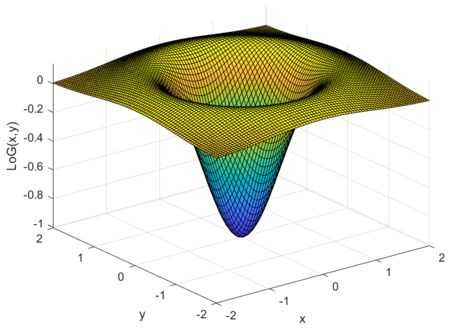
The Laplacian of Gaussian (LoG) operator of a 2D image is illustrated in Figure 1 and defined by [14]

Figure 1.
2D Laplacian of Gaussian operator (37) with .
Fractional grey-scale: In 2014, the authors of [4] presented a fractional adaptation for the first operator in (36) (using the symetric mask).
In a discrete function (f), the operator corresponds to approximation
Decomposing and noting that for this case, ,
By generalizing the order from integer to fractional, a fractional-order differential form of the Laplacian operator can be obtained:
Using the GL definition for the fractional-order derivative as it was used for the other operators, one may arrive at
With the definition above, the mask that performs the calculation of the fractional Laplacian may be built:
Experiments with (42) show that, the larger the order of differentiation is, the better the image feature is preserved, but the more noise that appears too.
Colour: A novel, colour-based, fractional LoG operator was implemented and tested in this study. The conventional algorithm finds edges searching for zero-crossings. This means that previous formulations cannot be adapted. According to [17], a pixel of a colour image is considered as part of an edge if zero-crossings are found in any of the colour channels. Thus, the fractional grey-scale operator formulated in [4] can be applied to each colour channel of a colour image. Then, a search for zero-crossings in the convolution outputs may be performed. If a zero-crossing is found in any of the channels, the corresponding pixel is flagged as part of an edge. The output of this algorithm is a binary image with all edges found.
2.7. CRONE
Original fractional grey-scale: In 2002, Benoît Mathieu wanted to prove that an edge detector based on fractional differentiation could improve edge detection and detection selectivity in the case of parabolic luminance transition.
The first derivative of a function , calculated with increasing x, can be defined by
with decreasing x,
with h being infinitesimally small.
A shift operator q is consequently introduced, defined by
Using the shift operator on the directional derivative yields
From the expressions above, it is clear that
Generalizing to an order n, and can be defined as
As explained before, the bidirectional detector can be constructed by a composition of the two unidirectional operators using the following expression:
Expanding and using Newton’s binomial formula, the expression above can be rewritten:
Applying the operator to a function, such as the transition studied before,
where
In order to detect edges on images, the formulated detector must be designed in two dimensions. Two independent vector operators for x and y, each of them a truncated CRONE detector, given respectively by
are used for this purpose. The detector was experimented in artificial and real images, and performance compared with Prewitt operators. In all cases, the CRONE detector showed better immunity to noise.
Colour: In this paper, a novel, colour-based, fractional CRONE was implemented, following the same steps as in the colour Canny already formulated. The colour channels are convolved with the masks for each direction constructing a Jacobian. Then, the maximum eigenvalue of is computed in order to find the pixels where the variation in chromatic image is higher than a designated threshold.
2.8. Fractional Derivative Operator
Original fractional grey-scale: In the fractional Roberts, the fractional mask is used in addition to the conventional integer mask. In this study, the Fractional Derivatives mask in (29) was implemented individually as a fractional edge detector.
Colour: A new colour-based version for this detector was also implemented. In this case, there is only one mask to detect edges in eight different directions. Thus, the Jacobian is reduced to a vector (one dimension):
The magnitude of the gradients was computed with the 3D vector formula:
3. Results
3.1. Implementation
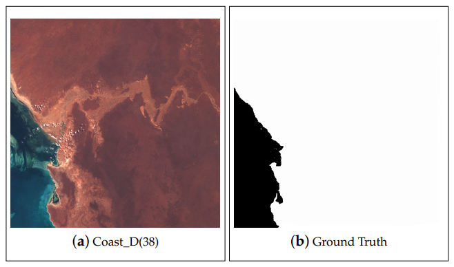
All edge detectors were implemented in MATLAB to perform fractional detection. A low-nebulosity image from ESA’s Sentinel-2 satellite [18] is used below to illustrate performance. The image retrieved from the website was analysed, and a ground truth was manually taken using GIMP. Both the selected photograph and its corresponding ground truth are given in Figure 2. Additional results for a greater number of images from the same source are available in Excel files from our public repository [10]. Performance was checked with the usual metrics
of which the first two are, respectively, the Jaccard coefficient and the Dice similarity coefficient. In (61)–(64), true-positives, false-positives, true-negatives, and false-negatives are defined as usual (see Table 1).

Figure 2.
Photograph used to illustrate performance and its ground truth.

Table 1.
Performance instances.
All the algorithms in Section 2 were tested with parameters varying within wide ranges (, , , ). The best performances of the different colour detectors are presented as an example in Figure 3; for additional examples, see the repository [10].
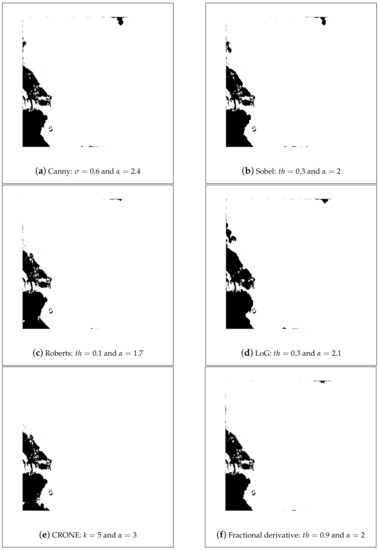
Figure 3.
Best results for Figure 2 processed using the different algorithms for colour images; is the threshold.
4. Discussion
Fractional-order adaptations of grey-scale edge detection algorithms are known to usually have better performance than the original method [19]. This happens in the example shown, where the results for Canny serve as an illustration: the integer algorithm achieves a Jaccard coefficient of 51.80%, the fractional method increases this result to 73.56%, and the colour version was able to almost entirely close the smooth inner-land gradients, achieving a Jaccard coefficient of 96.32%. Even when the increase in performance is low in percentage, since we are dealing with images that are composed of more than 120 million pixels, a 1% increase corresponds to more than one million correctly identified pixels. On the other hand, it is true that the colour-based detector is also heavier computationally, since it usually requires more than one convolution (at least one for each colour channel).
To summarize, in this study, seven novel fractional edge-detection methods were introduced (viz. one grey-scale and six colour-based versions). Future work includes a statistical assessment of their relative performance, in different types of images and applications, to statistically measure how their use improves performance.
Author Contributions
M.H.: methodology, software, investigation, data curation, writing—original draft preparation, visualization; D.V.: conceptualization, methodology, validation, investigation, writing—review and editing, supervision; P.G.: validation, investigation, writing—review and editing; R.M.: conceptualization, methodology, validation, investigation, data curation, writing—review and editing, supervision. All authors have read and agreed to the published version of the manuscript.
Funding
This work was supported by FCT, through IDMEC, under LAETA, project UIDB/50022/2020; by FCT under the ICT (Institute of Earth Sciences) project UIDB/04683/2020; and by FCT, through the CENTRA project UIDB/00099/2020.
Institutional Review Board Statement
Not applicable.
Informed Consent Statement
Not applicable.
Data Availability Statement
See [10].
Acknowledgments
The authors would like to acknowledge ESA, Copernicus for kindly providing access to the database for this research.
Conflicts of Interest
The authors declare no conflict of interest.
Abbreviations
The following abbreviations are used in this manuscript:
| Appears in | ||
| CRONE | Commande Robuste d’Order Non-Entier | Section 2.7 |
| (Non-integer order robust control, in French) | ||
| DSC | Dice similarity coefficient | Equation (62) |
| ESA | European Space Agency | Section 3.1 |
| FN | False negative | Table 1 |
| FP | False positive | Table 1 |
| GIMP | GNU Image Manipulation Program | Section 3.1 |
| GL | Grünwald-Letnikoff | Section 2.1 |
| LoG | Laplacian of Gaussian | Section 2.6 |
| TN | True negative | Table 1 |
| TP | True positive | Table 1 |
References
- Mathieu, B.; Melchior, P.; Oustaloup, A.; Ceyral, C. Fractional differentiation for edge detection. Signal Process. 2003, 83, 2421–2432. [Google Scholar] [CrossRef]
- Yaacoub, C.; Zeid Daou, R.A. Fractional Order Sobel Edge Detector. In Proceedings of the 2019 Ninth International Conference on Image Processing Theory, Tools and Applications (IPTA), Istanbul, Turkey, 6–9 November 2019; pp. 1–5. [Google Scholar] [CrossRef]
- Chen, X.; Fei, X. Improving edge-detection algorithm based on fractional differential approach. In Proceedings of the 2012 International Conference on Image, Vision and Computing, Shanghai, China, 25–26 August 2012; Volume 50. [Google Scholar] [CrossRef]
- Tian, D.; Wu, J.; Yang, Y. A Fractional-Order Laplacian Operator for Image Edge Detection. Appl. Mech. Mater. 2014, 536–537, 55–58. [Google Scholar] [CrossRef]
- Kanade, T. Image Understanding Research at Carnegie Mellon. In Proceedings of a Workshop on Image Understanding Workshop; Morgan Kaufmann Publishers Inc.: Los Angeles, CA, USA, 1987; pp. 32–48. [Google Scholar]
- Cumani, A. Edge detection in multispectral images. CVGIP Graph. Model. Image Process. 1991, 53, 40–51. [Google Scholar] [CrossRef]
- Valério, D.; da Costa, J.S. Introduction to single-input, single-output fractional control. IET Control Theory Appl. 2011, 5, 1033–1057. [Google Scholar] [CrossRef]
- Grünwald, A.K. Über “begrenzte” Derivationen und deren Anwendung. Z. FüR Math. Und Phys. 1867, 12, 441–480. [Google Scholar]
- Letnikov, A. Theory of Differentiation with an Arbitrary Index (Russian). Moscow Matem. Sbornik 1872, 6, 413–445. [Google Scholar]
- Henriques, M. Results Repository. Available online: https://drive.google.com/drive/folders/1GMeKvc3oqNWfzd4h-GyRwHT9yFJ_UDLP?usp=sharing (accessed on 15 January 2021).
- Canny, J. A computational approach to edge detection. IEEE Trans. Pattern Anal. Mach. Intell. 1986, 679–698. [Google Scholar] [CrossRef]
- CVonline. Edges: The Canny Edge Detector. Available online: http://homepages.inf.ed.ac.uk/rbf/CVonline/LOCAL_COPIES/MARBLE/low/edges/canny.htm (accessed on 31 July 2020).
- Koschan, A.; Abidi, M. Detection and classification of edges in color images. IEEE Signal Process. Mag. 2005, 22, 64–73. [Google Scholar] [CrossRef]
- Fisher, R.; Perkins, S.; Walker, A.; Wolfart, E. Image Processing Learning Resources. 2004. Available online: http://homepages.inf.ed.ac.uk/rbf/HIPR2/ (accessed on 15 January 2021).
- Roberts, L. Machine Perception of 3-D Solids. Ph.D. Thesis, Massachusetts Institute of Technology, Cambridge, MA, USA, 1963. [Google Scholar]
- Pratt, W.K. Second-Order Derivative Edge Detection. In Digital Image Processing; John Wiley & Sons, Inc.: Hoboken, NJ, USA, 2007. [Google Scholar] [CrossRef]
- Zhu, S.Y.; Plataniotis, K.N.; Venetsanopoulos, A.N. Comprehensive analysis of edge detection in color image processing. Opt. Eng. 1999, 38, 612–625. [Google Scholar] [CrossRef]
- ESA. Copernicus Open Access Hub. 2020. Available online: https://scihub.copernicus.eu/ (accessed on 31 March 2020).
- Bento, T.; Valério, D.; Teodoro, P.; Martins, J. Fractional order image processing of medical images. J. Appl. Nonlinear Dyn. 2017, 6, 181–191. [Google Scholar] [CrossRef]

Publisher’s Note: MDPI stays neutral with regard to jurisdictional claims in published maps and institutional affiliations. |
© 2021 by the authors. Licensee MDPI, Basel, Switzerland. This article is an open access article distributed under the terms and conditions of the Creative Commons Attribution (CC BY) license (http://creativecommons.org/licenses/by/4.0/).