High-Precision Kriging Modeling Method Based on Hybrid Sampling Criteria

Abstract

Finding new valuable sampling points and making these points better distributed in the design space is the key to determining the approximate effect of Kriging. To this end, a high-precision Kriging modeling method based on hybrid sampling criteria (HKM-HS) is proposed to solve this problem. In the HKM-HS method, two infilling sampling strategies based on MSE (Mean Square Error) are optimized to obtain new candidate points. By maximizing MSE (MMSE) of Kriging model, it can generate the first candidate point that is likely to appear in a sparse area. To avoid the ill-conditioned correlation matrix caused by the too close distance between any two sampling points, the MC (MSE and Correlation function) criterion formed by combining the MSE and the correlation function through multiplication and division is minimized to generate the second candidate point. Furthermore, a new screening method is used to select the final expensive evaluation point from the two candidate points. Finally, the test results of sixteen benchmark functions and a house heating case show that the HKM-HS method can effectively enhance the modeling accuracy and stability of Kriging in contrast with other approximate modeling methods.

1. Introduction

In the field of engineering design and scientific practice, simulation models are widely used to imitate and analyze expensive black box problems. The rapid development and advancement of technology makes some black box problems have greater nonlinearity and computational complexity. Therefore, the simulation models will undoubtedly become more complex and the computing cost will be more expensive. All of these bring additional challenges to the black box simulation problems. Under these circumstances, approximate models, especially for the surrogate models [1,2] (also known as meta-models or response surfaces), are widely applied to better simulate complex black box problems. Using surrogate models to approximately replace expensive simulations can not only significantly reduce the time spent, but also effectively improve the modeling accuracy.

Due to the actual demand of engineering and science, different types of surrogate models have sprung up. The classics mainly include Support Vector Regression (SVR) [3,4], Polynomial Response Surface (PRS) [5,6], Radial Basis Function (RBF) [7,8], Multiple Adaptive Regression Spline (MARS) [9] and Kriging [10,11,12]. The PRS model can solve low-order, low-dimensional and easy-to-access engineering design problems. However, it is not suitable for solving high-dimensional nonlinear multi-modal design problems. RBF is an interpolation method that uses the sum of the weights of the basic functions to approximate complex black box problems. The RBF method can more accurately approximate nonlinear and high-dimensional black box problems, but the approximate requires it to use more function evaluations, which in turn increases the time cost. The computational complexity of the SVR model depends on the number of support vectors rather than the dimension of the sample space. In this way, the dimension problem can be avoided. However, the time cost of the SVR model is relatively high, and it is difficult to handle the problem of large-scale training samples. MARS is a nonlinear nonparametric regression method which can use piecewise linear splines to simulate the relationship between the dependent and independent variables and has good adaptability. However, with the expansion of the sample space, the MARS method is difficult to divide the space effectively, and the recursive partitioning makes the model lack continuity. In the high-dimensional case, it does not have the ability to capture relatively simple functional relationships. However, the Kriging model always has good approximation properties. The reason is that Kriging model not only has smaller errors and higher accuracy, but also can handle linear or nonlinear, simple or complex, low-dimensional or high-dimensional problems. Secondly, the Kriging can estimate the uncertainty of the model, and its basis function usually has adjustable parameters. Moreover, the Kriging model can ensure the smoothness of the function and has high execution efficiency and good accuracy. These excellent properties make the Kriging model popular. Craven et al. applied the Kriging surrogate model to medicine, in which Kriging has a good effect on predicting the power law coefficient of hemolysis [13]. Song et al. applied the Kriging surrogate model to the layout design of Vortex-Induced Piezoelectric Energy Converters (VIPECs) [14]. Yu et al. applied the Kriging model to the tip leakage flow control of the multi-stage DBD (dielectric barrier discharge) plasma actuator blade cascade [15]. The Kriging method can increase the efficiency of permanent magnet synchronous generators (PMSG) for vehicles [16].

Although the Kriging model shows superior performance and has been successfully applied in various fields, there are still some problems in the Kriging model that need to be further studied [17]. The specific problems are as follows. (1) The infilling sampling criterion will affect the approximation accuracy of the Kriging model. How to find a good infilling sampling strategy to select the next sampling point is the core of the iterative process of the adaptive sequence experiment design method based on Kriging. (2) What are the internal relationships between the accuracy of the Kriging model and its eight kernel functions? (3) How to determine the best applicable field of each kernel function is an issue that needs attention. We mainly discuss the construction problem of infilling sampling criterion for Kriging in this work.

A good sampling strategy can directly enhance the accuracy and efficiency of the surrogate model, which is very helpful for solving computationally expensive simulation systems and complex engineering design problems. Therefore, many scholars put forward the sampling strategy of the Kriging model and applied it to the modeling process of the Kriging model. Among them, the adaptive sampling strategy based on active learning [18] has received more and more attention in recent years. The next update point of the simplest adaptive sampling strategy is selected according to the maximum mean square error (MMSE) [19]. The MMSE method is widely used because of its high accuracy and low calculation time. An adaptive sampling method in the framework of bias-variance decomposition was proposed in [20]. The sampling criterion of this method is to maximize the expected prediction error of the bias and variance information to select the sampling point. An adaptive Bayesian sequential sampling method was proposed in [21], which determines the new sampling point by maximizing the determinant of the adjusted covariance matrix. Sacks et al. select new points by maximizing the expected reduction in integrated mean square error (IMSE) in the entire design space [22]. Ping proposed a Kriging meta-model adaptive sampling strategy (KMDT) based on Delaunay triangulation and TOPSIS [23]. In addition, there is also the maximum entropy sampling method (ME) [24], parallel adaptive sampling strategy (PAS) [25], maximum curvature minimum distance sequence sampling [26], etc. These are all effective methods to increase the update points, but these methods are limited to adding a new sample point in one iteration cycle and cannot use more computer resources to improve the calculation efficiency.

To generate multiple sampling points in each cycle, a multi-point plus point strategy was presented by considering the predicted response value and uncertainty of the Kriging model. A multi-point sampling strategy based on Kriging (MPSK) was presented in [27]. This strategy assumes that every unobserved point in the region may be the next update point. During the sampling process, the expected improvement function is transformed into a cumulative probability distribution function, and an appropriate new sample is intelligently drawn within a certain probability region. In addition, Li proposed a Kriging-based multi-point sequential sampling optimization (KMSSO) method [28]. So far, there are few relevant literatures and research results to solve this problem. The reasons for this phenomenon are as follows. When adding multiple points at the same time, the correlation between each point needs to be considered, otherwise it may lead to an ill-conditioned matrix, or find the same point and cause modeling failure. Adding multiple points at the same time may take too much time, resulting in low modeling efficiency. Adding multiple points at the same time does not guarantee that each point is promising and may fail to improve the accuracy.

To overcome this bottleneck problem, a high-precision Kriging modeling method based on hybrid sampling criteria (HKM-HS) is proposed. Two sampling strategies, MMSE and MC, are included in HKM-HS. First, the MMSE sampling strategy is used to generate the first candidate point. If the second candidate point is directly generated by MMSE, the distance between the two candidate points may be very close, resulting in the ill-conditioned correlation matrix. Therefore, the correlation function is added as a selection condition when selecting the second candidate point. MMSE is to ensure that the candidate points have the maximum amount of information, while the minimum correlation function is to ensure that the distance between the candidate points and the existing sample points is not too close, thereby ensuring that the new correlation matrix will not be ill-conditioned. The MC criterion is obtained by combining the maximum mean square error and the minimum correlation function through the multiplication and division method, and the second candidate point is obtained by MC sampling criterion. Finally, the evaluation points are selected from two candidate points.

The rest of this work is organized as follows. The second part discusses the basic background of the Kriging model. The third part proposes two sampling criteria and gives specific steps for determining new sampling points. The fourth part tests 16 benchmark functions and two actual cases and gives the test results. The fifth part is the application of HKM-HS method in house heating. The sixth part is the conclusion.

2. Related Work

2.1. Kriging

In statistics, the interpolation process of Kriging is finished by a Gaussian process controlled by the priori covariance. Under appropriate a priori assumptions, the Kriging model can provide the best linear unbiased prediction. The specific details are stated as follows.

Suppose there are m sample points $X={\left[{\mathit{x}}_1,\dots ,{\mathit{x}}_m\right]}^T$, $X\in {\Re }^{m\times n}$ and object response $Y={[{\mathit{y}}_1,\dots , {\mathit{y}}_m]}^{\mathrm{T}}$. The Kriging model is expressed as follows.

$$y(\mathit{x})=\mu (\mathit{x})+z(\mathit{x})$$

(1)

The Equation consists of two parts. The first part $\mu (\mathit{x})$ is the trend function. When $\mu (\mathit{x})$ is equal to 0, $\mu$ and ${\displaystyle {\sum }_{i=1}^p{\beta }_i{f}_i(\mathit{x})}$ are called simple Kriging, ordinary Kriging, and standard Kriging models, respectively. Where $f_i(\mathit{x})$ and ${\beta }_i$ are the regression function and the corresponding regression function coefficients, respectively. Standard Kriging uses the regression function to determine the change of process mean [29].

The second part of Equation (1) is a stochastic process model established by observing the data and quantifying the correlation of data. $z\left(\mathit{x}\right)$ is considered as the realization of the stochastic process $Z\left(\mathit{x}\right)$ with mean of 0 and variance of ${\sigma }^2$. The covariance between sampling points is shown in Equation (2).

$$E\left[Z\left({\mathit{x}}_i\right)Z\left({\mathit{x}}_j\right)\right]={\sigma }^{2}R\left(\mathit{\theta },{\mathit{x}}_i,{\mathit{x}}_j\right)$$

(2)

where process variance ${\sigma }^2$ is a scalar and $\mathit{\theta }$ is a key parameter of the kernel function. By optimizing $\mathit{\theta }$, the correlation between the design points can be adjusted adaptively. The expression of the kernel function is as follows.

$$R\left(\mathit{\theta },{\mathit{x}}_i,{\mathit{x}}_j\right)={\displaystyle \prod _{k=1}^n{R}_k\left({\theta }_k,x_i^k-x_j^k\right)}$$

(3)

There are many options for spatial correlation functions. However, the most widely used correlation function is the Gaussian function. The expression of the Gaussian model is as follows.

$$R_k\left({\theta }_k,x_i^k-x_j^k\right)=\exp \left(-{\theta }_k{\left|x_i^k-x_j^k\right|}^2\right)$$

(4)

Under the above assumptions, the best linear unbiased estimate of $y\left(\mathit{x}\right)$ is

$$\widehat{y}\left(\mathit{x}\right)={\mathit{f}}^T\left(\mathit{x}\right)\widehat{\mathit{\beta }}+{\mathit{r}}^T\left(\mathit{x}\right)R^{-1}\left(\mathbf{Y}-F\widehat{\mathit{\beta }}\right)$$

(5)

$\mathit{r}$ and $R$ in Equation (5) are

$$\mathit{r}\left(\mathit{x}\right)=\left\{R\left(\mathit{\theta },\mathit{x},{\mathit{x}}_1\right),R\left(\mathit{\theta },\mathit{x},{\mathit{x}}_2\right),\cdots ,R\left(\mathit{\theta },\mathit{x},{\mathit{x}}_m\right)\right\}$$

(6)

$$R_{m\times m}=\left[\begin{array}{ccc}R\left(\mathit{\theta },{\mathit{x}}_1,{\mathit{x}}_1\right)& \cdots & R\left(\mathit{\theta },{\mathit{x}}_1,{\mathit{x}}_m\right)\\ ⋮& \ddots & ⋮\\ R\left(\mathit{\theta },{\mathit{x}}_m,{\mathit{x}}_1\right)& \cdots & R\left(\mathit{\theta },{\mathit{x}}_m,{\mathit{x}}_m\right)\end{array}\right]$$

(7)

Among them, the least square estimation $\widehat{\mathit{\beta }}$ of $\mathit{\beta }$ can be obtained by calculating Equation (8).

$$\widehat{\mathit{\beta }}={\left(F^T{R}^{-1}F\right)}^{-1}{F}^T{R}^{-1}Y$$

(8)

In addition, the predicted mean square error $\widehat{s}\left(\mathit{x}\right)$ of $\widehat{y}\left(\mathit{x}\right)$ can be calculated by Equation (9).

$$\widehat{s}\left(\mathit{x}\right)=MSE\left[\widehat{y}\left(\mathit{x}\right)\right]={\widehat{\sigma }}^2\left\{1-\left[\mathit{f}{\left(\mathit{x}\right)}^T\hspace{0.17em}\hspace{0.17em}\mathit{r}{\left(\mathit{x}\right)}^T\right]\left[\begin{array}{cc}\mathit{0}& F^T\\ F& R\end{array}\right]\left[\begin{array}{c}\mathit{f}\left(\mathit{x}\right)\\ \hspace{0.17em}\mathit{r}\left(\mathit{x}\right)\end{array}\right]\right\}$$

(9)

where

$${\widehat{\sigma }}^2=\frac{1}{m}{\left(Y-F\widehat{\mathit{\beta }}\right)}^T{R}^{-1}\left(Y-F\widehat{\mathit{\beta }}\right)$$

(10)

It can be seen from Equations (3), (8) and (9) that the matrix $R$, vector $\widehat{\mathit{\beta }}$, and the estimated variance $\widehat{s}\left(\mathit{x}\right)$ of the unknown point all depend on the value of the parameter $\mathit{\theta }$. Based on the maximum likelihood estimation theory, the unconstrained optimization algorithm is used to maximize Equation (11) to obtain the optimal $\mathit{\theta }$ value [30].

$$\mathit{\theta }=\arg \max \left(-\frac{m}{2}\ln {\widehat{\sigma }}^2-\frac{1}{2}\ln \left|R\right|\right)$$

(11)

In fact, the best approximation curve is not necessarily obtained from the optimal value, as long as the value is close to the optimal value, there will be a good approximation result.

2.2. AME

The AME (adaptive maximum entropy) [21] sampling method determines the new sampling point by maximizing the determinant of the adjusted covariance matrix. The adjusted covariance matrix expression is as follows.

$$\mathrm{cov}({\mathit{x}}_i,{\mathit{x}}_j)={\sigma }^2{\displaystyle \prod _{k=1}^n\exp (-{\eta }_i{\eta }_j{\theta }_k{\left|d_k\right|}^2)}={\sigma }^2{\displaystyle \prod _{k=1}^n\exp (-{\left(\frac{e_i}{e_{\max }}\right)}^{\gamma }{\left(\frac{e_j}{e_{\max }}\right)}^{\gamma }{\theta }_k{\left|d_k\right|}^2)}$$

(12)

where ${\eta }_i$ and ${\eta }_j$ are the adjust factors for points ${\mathit{x}}_i$ and ${\mathit{x}}_j$, respectively. They are determined by the errors at ${\mathit{x}}_i$ and ${\mathit{x}}_j$. The parameter $\gamma$ can be adjusted to ${\eta }_i$ to balance local exploitation and global exploration. The adjusted covariance matrix not only considers the distance factor between two points, but also considers the error of the two points. Sampling more points in the area with a larger error can improve the accuracy of the meta-model.

When ${\mathit{x}}_i$ is a known sample point, $e_i=\left|y({\mathit{x}}_i)-\widehat{y}({\mathit{x}}_i)\right|$. When ${\mathit{x}}_i$ is the unsampled point, $e_i=\left|y({\mathit{x}}_j)-\widehat{y}({\mathit{x}}_j)\right|$, where ${\mathit{x}}_j$ is the sampled point closest to ${\mathit{x}}_i$.

3. HKM-HS Method

The purpose of this paper is to add one or two new sampling points in an optimization iteration of the Kriging model. The HKM-HS method with two infilling sampling criteria can achieve this purpose. The specific details of the two infilling sampling criteria are as follows.

3.1. Maximizing Mean Square Error (MMSE)

A good sampling criterion can not only improve the accuracy and efficiency of modeling, but also reduce the cost of modeling. The criterion for evaluating the merits and demerits of the sampling methods are as follows. Whether the newly discovered sampling points have more information in the design field and whether the sampling points can be more evenly distributed in the entire design space under the premise of maintaining certain independence has yet to be determined. The common sampling criteria are maximum mean square error (MMSE), integrated mean square error (IMSE) [22], an adaptive Bayesian sequential sampling method [21] and maximum entropy sampling method (ME) [24]. The ME method tends to add candidate points far away from the current sample points, without considering the objective information of the design point. The adaptive Bayesian sequential sampling method considers not only the distance factor but also the error factor when adding design points, but the running time is slightly longer than the MMSE and IMSE methods. Both MMSE and IMSE methods can obtain the next sampling point by combining the known sample data with the Kriging model. The ideas of the two methods are similar, but the MMSE method is simpler and easier. The MMSE method can obtain sampling points with potentially useful information from the current Kriging model. In the sampling process, the distance between sampling points is considered to ensure that the new sampling data is evenly distributed in the entire design space. Therefore, MMSE sampling criterion is selected as the final sampling criterion. The established model is as follows.

$$\max \hspace{0.17em}{f}_1\left(\mathit{x}\right)=\widehat{s}\left(\mathit{x}\right)$$

(13)

where $\widehat{s}\left(\mathit{x}\right)={\widehat{\sigma }}^2\left\{1-\left[\mathit{f}{\left(\mathit{x}\right)}^T\hspace{0.17em}\hspace{0.17em}\mathit{r}{\left(\mathit{x}\right)}^T\right]\left[\begin{array}{cc}0& F^T\\ F& R\end{array}\right]\left[\begin{array}{c}\mathit{f}\left(\mathit{x}\right)\\ \hspace{0.17em}\mathit{r}\left(\mathit{x}\right)\end{array}\right]\right\}$ is a function about the unknown point $\mathit{x}$. The purpose of Equation (13) is to find the candidate point $\mathit{x}$ when the mean square error is maximized.

3.2. MC Criterion

The spatial correlation function (SCF) can affect the smoothness of the Kriging model. This correlation applies to not only the known sample points, but also to the quantified observations. There are eight commonly used correlation function models in SCF [31,32,33]. See

Table 1. Expressions of different correlation functions.

$\mathbf{Spatial} \mathbf{Correlation} \mathbf{Function} \mathbf{Model} {\mathit{R}}_{\mathit{k}}\left({\mathit{\theta }}_{\mathit{k}},{\mathit{d}}_{\mathit{k}}\right)$$, \mathbf{where} {\mathit{d}}_{\mathit{k}}={\mathit{x}}_{\mathit{i}}^{\mathit{k}}-{\mathit{x}}_{\mathit{j}}^{\mathit{k}}$
Exponential model	$R_k\left({\theta }_k,d_k\right)=\exp \left(-{\theta }_k\left|d_k\right|\right)$
Exponential Gaussian model	$R_k\left({\theta }_k,d_k\right)=\exp \left(-{\theta }_k{\left|d_k\right|}^{{\theta }_{n+1}}\right),{\theta }_{n+1}\in \left(0,2\right]$
Gaussian model	$R_k\left({\theta }_k,d_k\right)=\exp \left(-{\theta }_k{\left|d_k\right|}^2\right)$
Linear model	$R_k\left({\theta }_k,d_k\right)=\max \left(0,1-{\theta }_k\left|d_k\right|\right)$
Spherical model	$R_k\left({\theta }_k,d_k\right)=1-1.5{\epsilon }_k+0.5{\epsilon }_k,\hspace{0.17em}\hspace{0.17em}\hspace{0.17em}{\epsilon }_k=\min \left\{1,{\theta }_k\left|d_k\right|\right\}$
Cubic model	$R_k\left({\theta }_k,d_k\right)=1-3{\epsilon }_k^2+2{\epsilon }_k^3,\hspace{0.17em}\hspace{0.17em}\hspace{0.17em}{\epsilon }_k=\min \left\{1,{\theta }_k\left|d_k\right|\right\}$
Spline model	$R_k\left({\theta }_k,d_k\right)=\left\{\begin{array}{cc}1-15{\epsilon }_k^2+30{\epsilon }_k^3,\hspace{0.17em}\hspace{0.17em}\hspace{0.17em}& {\epsilon }_k\in \left(0,0.2\right]\\ 1.25{\left(1-{\epsilon }_k\right)}^3,\hspace{0.17em}\hspace{0.17em}\hspace{0.17em}& {\epsilon }_k\in \left(0.2,1\right)\\ 0,& {\epsilon }_k\in \left[1,\infty \right)\end{array}\right.$
Matérn model	$R_k\left({\theta }_k,d_k\right)=\left(1+\sqrt{3}{\theta }_k\left|d_k\right|\right)\exp \left(-\sqrt{3}{\theta }_k\left|d_k\right|\right)$

for details.

The following is an example to prove the advantages of the Gaussian correlation function. A simple one-dimensional problem is expressed as [25]:

$$f(x)={(6x-2)}^2\sin \left(12x-4\right)\hspace{0.17em}\hspace{0.17em}\hspace{0.17em}\hspace{0.17em}\hspace{0.17em}\hspace{0.17em}x\in \left[0,1\right]$$

Different correlation functions are used in Kriging modeling process. Figure 1 shows the trend and error of the approximate function.

AE (absolute error) in Figure 1b is the absolute error between the actual value and the predicted value. The Figure 1a shows the relationship between the original function and the seven Kriging approximate functions based on different correlation functions. The approximate results show that the selection of correlation function does have a certain influence on the accuracy of the Kriging modeling and the selection of new samples. When the kernel function of the Kriging is the Gaussian function, the approximate function is closest to the original function. Figure 1b indicates that the Kriging approximation function with Gaussian kernel function has the smallest error, which shows that the Kriging approximation function has the highest prediction accuracy.

To further verify the effectiveness of the Gaussian kernel function, a three-dimensional function and a five-dimensional function are used as examples to verify it. Figure 2a,b are graphs of the average absolute error of each experiment run 20 times. Obviously, the Kriging model based on the Gaussian kernel function has the smallest average absolute error, which proves the effectiveness of the Gaussian kernel function.

$$f(\mathit{x})=(x_3+2)x_2{x}_1^2\hspace{0.17em}\hspace{0.17em}\hspace{0.17em}\hspace{0.17em}\hspace{0.17em}\hspace{0.17em}{x}_i\in \left[0,2\right]$$

$$f(\mathit{x})=\sqrt{2}\left(x_1+x_2+x_3+x_4+x_5\right)\hspace{0.17em}\hspace{0.17em}\hspace{0.17em}\hspace{0.17em}\hspace{0.17em}\hspace{0.17em}{x}_i\in \left[0,1\right]$$

When comparing the effectiveness of multiple kernel functions, the Exponential Gaussian kernel function does not participate in the comparison. There are two main reasons. One is that the specific expression varies according to the parameter ${\theta }_{n+1}$, so there is no fixed expression. The other is that the Exponential kernel function and the Gaussian kernel function are both special forms of the Exponential Gaussian kernel function; that is, the exponential kernel and the Gaussian kernel belong to the Exponential Gaussian kernel.

According to these analyses, the Gaussian kernel function is finally selected as the correlation function. Its specific expression is shown in Equation (4).

$$R_k\left({\theta }_k,x_i^k-x_j^k\right)=\exp \left(-{\theta }_k{\left|x_i^k-x_j^k\right|}^2\right)$$

The smaller the correlation between the new sampling point and the known sampling points, the better. If the correlation value is large, the matrix $R$ may be ill-conditioned. In view of this, the requirement of minimizing the correlation function in Equation (13) need be met to minimize the correlation between new sampling points and all design points.

$$\min \hspace{0.17em}\hspace{0.17em}\hspace{0.17em}\hspace{0.17em}\hspace{0.17em}\hspace{0.17em}{f}_2\left(\mathit{x}\right)=\sqrt{r_1^2+\cdots +r_m^2}$$

(14)

where parameter $r_i=R\left(\mathit{\theta },\mathit{x},{\mathit{x}}_i\right)\hspace{0.17em}\hspace{0.17em}\hspace{0.17em}\hspace{0.17em}\hspace{0.17em}i=1,\dots ,m$ is the correlation between new sampling point and the $i$th sample point.

Multiplication and division can be used to deal with multi-objective optimization problems [34,35]. The multiplication or division of multiple objective optimization functions can make multi-objective optimization problems have a clearer meaning and can transform the multi-objective optimization problem into a single-objective optimization problem, so that the single-objective contains the optimization intent of each single objective in the multi-objective. If multiple objective functions need to be maximized, we can multiply them together to form a new objective function $f\left(x\right)=f_1\left(x\right)·f_2\left(x\right)\cdots f_k\left(x\right)$; or we can use a weighted geometric mean to construct a new objective function, such as $f\left(x\right)={\left[f_1\left(x\right)\right]}^{{\alpha }_1}·{\left[f_2\left(x\right)\right]}^{{\alpha }_2}\cdots {\left[f_k\left(x\right)\right]}^{{\alpha }_k}$, where ${\alpha }_i\ge 0,1\le i\le k,{\displaystyle \sum _{i=1}^k{\alpha }_i}=1$. If some of the multiple objective functions need to be maximized and others need to be minimized, the product of all objective functions to be maximized can be divided by the product of all objective functions that are minimized and then maximized, or the product of all the objective functions that need to be minimized is divided by the product of all the objective functions to be maximized and then minimized, and so on. In this way, the problem can be transformed into a problem of maximizing or minimizing the value in the form of “multiplication and division.” For the problems raised in this paper, we can get the following single-objective optimization model:

$$\min \hspace{0.17em}\hspace{0.17em}\hspace{0.17em}\hspace{0.17em}\hspace{0.17em}\hspace{0.17em}G\left(\mathit{x}\right)=\frac{f_2\left(\mathit{x}\right)}{f_1\left(\mathit{x}\right)}=\frac{{\widehat{\sigma }}^2\left\{1-\left[\mathit{f}{\left(\mathit{x}\right)}^T\hspace{0.17em}\hspace{0.17em}\hspace{0.17em}\hspace{0.17em}\hspace{0.17em}\mathit{r}{\left(\mathit{x}\right)}^T\right]\left[\begin{array}{cc}0& F^T\\ F& R\end{array}\right]\left[\begin{array}{c}\mathit{f}\left(\mathit{x}\right)\\ \hspace{0.17em}\mathit{r}\left(\mathit{x}\right)\end{array}\right]\right\}}{\sqrt{r_1^2+\cdots +r_m^2}}$$

(15)

where $f_1\left(\mathit{x}\right)$ represents the mean square error function, as shown in Equation (13); $f_2\left(\mathit{x}\right)$ represents the correlation function, as shown in Equation (14). Equation (15) is obtained by combining the two objective functions of Equations (13) and (14) through multiplication and division. The significance of building model (15) is to transform two objective functions into a single objective function.

The range of each $r_i\left(i=1,\dots ,m\right)\hspace{0.17em}$ in function $f_2$ is $\left[0,\hspace{0.17em}1\right]$, the corresponding range of $f_2$ is $\left[0,\hspace{0.17em}\sqrt{m}\hspace{0.17em}\right]$. The range of $f_1$ cannot be determined because the MSE of different functions is different, but the value of $f_1$ is always greater than 0.

In addition, the following situations may exist. When the range of $f_1$ is much smaller than that of $f_2$, a small change of the function $f_1$ will greatly affect the optimization results. In this situation, the function $f_1$ plays a leading role, and the selection of point pays more attention to the correlation between candidate point and all sample points. Similarly, when the range of $f_1$ is much bigger than that of $f_2$, the function $f_2$ dominates the optimization results, and the selection of point pays more attention to the amount of information of the candidate points. In either case, the point found can be used as a candidate point. Therefore, Equation (15) can be optimized directly. The optimal value obtained at this time is the second candidate sampling point.

3.3. Screening Method

Two candidate sampling points were generated through two infilling sampling criteria. In this paper, the PSO (particle swarm optimization) algorithm of MATLAB was used to optimize the sampling criteria. The first candidate point ${\mathit{x}}_i$ was obtained by optimizing the MMSE function (Equation (13)) through the PSO algorithm. The second candidate point ${\mathit{x}}_j$ was obtained by optimizing the $G\left(\mathit{x}\right)$ function (Equation (15)) with the PSO algorithm. Then, one or two candidate sampling points were selected as new sampling points. The method of selecting sampling points is described as follows.

First, set the correlation threshold to 0.001. The range of correlation is $\left[0,\hspace{0.17em}1\right]$. The closer the correlation value is to 0, the higher the mutual independence between the two points. Similarly, the closer the correlation value is to 1, the lower the mutual independence between the two sample points. In addition, the distance between two points with low independence may be too close, resulting in an ill-conditioned correlation matrix. Set the correlation threshold to 0.001, which is a value close enough to 0. This setting can ensure that the two candidate points have independent information and avoids the appearance of an ill-conditioned correlation matrix, which may lead to the consequences of modeling failure.

Second, determine the correlation value between two candidate points. The correlation value between two candidates ${\mathit{x}}_i$ and ${\mathit{x}}_j$ is determined by Gaussian correlation function. If the correlation value is less than 0.001, it means that the correlation between the two candidates ${\mathit{x}}_i$ and ${\mathit{x}}_j$ is very small. At this time, both ${\mathit{x}}_i$ and ${\mathit{x}}_j$ are selected as new sampling points. If the correlation value is equal to or greater than 0.001, it means that the correlation between the two candidates ${\mathit{x}}_i$ and ${\mathit{x}}_j$ is large. At this time, if both ${\mathit{x}}_i$ and ${\mathit{x}}_j$ are selected as new sampling points, the correlation matrix may be ill-conditioned. Therefore, in this case, select the point with large mean square error as the new sampling point.

3.4. Implementation of the HKM-HS Method

This section introduces the specific implementation process of the HKM-HS model.

Table 2. The specific steps of high-precision Kriging modeling method based on hybrid sampling criteria (HKM-HS).

HKM-HS Method

Step 1. Generate initial design points. The LHD (Latin Hypercube Design) method is used to generate $m=2n$ initial design point ${\mathit{x}}_i(i=1,\dots ,m)$. Then, set the initial sample set to $X$. Step 2. Determine the sample sets $X$ and $Y$. Estimate the expensive objective function of each initial sample point ${\mathit{x}}_i(i=1,\dots ,m)$ to obtain $y({\mathit{x}}_i)$. Then, set $Y$ to be the set of all $y({\mathit{x}}_i)$. For one or two update points obtained by the infilling sampling criterion, their expensive function evaluation values can be determined. Then the update point and its function evaluation value are added to the sample sets $X$ and $Y$, respectively. If there is only one new sampling point, then $m=m+1$; if there are two new sampling points, then $m=m+2$. Step 3. Build Kriging model. The Kriging model will be established by the new data sets $X$ and $Y$ formed by Step 2, and the construction of Kriging is realized by DACE toolbox in MATLAB. Step 4. Infill sampling criteria. The new infilling sampling method has two criteria, one is MMSE and the other is the MC sampling strategy based on mean square error and correlation function. See Section 3.1 and Section 3.2 for details. The PSO algorithm of MATLAB is used to optimize the sampling criteria. The first candidate point ${\mathit{x}}_i$ is obtained by optimizing the MMSE function (Equation (12)) through PSO algorithm. The second candidate point ${\mathit{x}}_j$ is obtained by optimizing the $G\left(\mathit{x}\right)$ function (Equation (14)) with PSO algorithm. Step 5. Determine new sampling point. First, two candidate sampling points ${\mathit{x}}_i$ and ${\mathit{x}}_j$ are generated with the new infilling sampling criteria. Then, one or two candidate sampling points are selected as new sampling points. See Section 3.3 for details. Step 6. Stopping criterion. The maximum number of function evaluations is set as $N_{\max }=20n$. Determine the relationship between m and $N_{\max }$. If the number of sampling points $m$ is greater than $N_{\max }$, stop adding points and go to step 7. If the condition is not met, go back to step 2. Step 7. Stop. This is the output global approximate Kriging model.

shows the specific implementation steps of the HKM-HS model.

Table 3. The pseudocode of HKM-HS.

Algorithm for HKM-HS

1. Begin 2. X and $Y$: Use LHD to generate m initial sample points and perform expensive functional evaluation on them. 3. Update $X$ and $Y$: Add the new sample point ${\mathit{x}}_i$ to $X$, and add $y({\mathit{x}}_i)$ to $Y$. 4. Update m: $m=m+1$ or $m=m+2$. $5. y\left(\mathit{x}\right)$$\text{:}$The Kriging is established with new sets X and $Y$. $6. {\mathit{x}}_i$ and ${\mathit{x}}_j$: Optimize the MMSE function and $G\left(\mathit{x}\right)$ function by PSO. 7. New sampling points: Screening method (Section 3.3). $8. \mathrm{If} m\text{<}20n$ Return to line 3or elsestop if this is the end. 9. End

is the pseudocode of the HM-HS algorithm. Figure 3 is the flowchart of the HKM-HS model.

4. Numerical Experiment

To test the modeling accuracy and stability of the HKM-HS method, the 16 benchmark functions were tested with HKM-HS, MMSE, LHD and AME [21] methods, respectively, and the test results of the four methods were compared. Then the HKM-HS algorithm was applied to the problems of spring design, simple pendulum system and a house heating case.

4.1. Benchmark Function Test

In this paper, a total of 16 benchmark functions were tested, and the dimensional range of these functions was 2 to 16 dimensions. Among them, there were 6 two-dimensional benchmark functions. Descriptions of these functions can be found in

Table 4. Benchmark functions.

Function	Dimension	Expression
Alpine	2	$y=\left|x_1\sin (x_1)+0.1x_1\right|+\left|x_2\sin (x_2)+0.1x_2\right|\hspace{0.17em}\hspace{0.17em}\hspace{0.17em}\hspace{0.17em}\hspace{0.17em}\hspace{0.17em}{x}_i\in \left[-10,10\right],i=1,2$
Bukin	2	$y=100\sqrt{\left|x_2-0.01x_1^2\right|}+0.01\left|x_1+10\right|\hspace{0.17em}\hspace{0.17em}\hspace{0.17em}\hspace{0.17em}\hspace{0.17em}\hspace{0.17em}{x}_1\in \left[-15,-5\right],x_2\in \left[-3,3\right]$
Gp	2	$\begin{array}{c}y=\left(30+{\left(2x_1-3x_2\right)}^2\left(18-32x_1+12x_1^2+48x_2-36x_1{x}_2+27x_2^2\right)\right)·\\ \hspace{0.17em}\hspace{0.17em}\hspace{0.17em}\hspace{0.17em}\hspace{0.17em}\hspace{0.17em}\left(1+{\left(x_1+x_2+1\right)}^2\left(19-14x_1+3x_1^2-14x_2+6x_1{x}_2+3x_2^2\right)\right)\hspace{0.17em}\hspace{0.17em}\hspace{0.17em}\hspace{0.17em}\hspace{0.17em}\hspace{0.17em}{x}_i\in \left[-2,2\right],i=1,2\end{array}$
Mccormick	2	$y=\sin \left(x_1+x_2\right)+{\left(x_1-x_2\right)}^2-1.5x_1+2.5x_2+1\hspace{0.17em}\hspace{0.17em}\hspace{0.17em}\hspace{0.17em}\hspace{0.17em}\hspace{0.17em}{x}_1\in \left[-1.5,4\right],x_2\in \left[-3,4\right]$
Schwefel	2	$y=837.9658-{\displaystyle \sum _{i=1}^2{x}_i\sin \left(\sqrt{\left|x_i\right|}\right)}\hspace{0.17em}\hspace{0.17em}\hspace{0.17em}\hspace{0.17em}\hspace{0.17em}{x}_i\in \left[-500,500\right],i=1,2$
sixHump	2	$y=4x_1^2-2.1x_1^4+x_1^6/3+x_1{x}_2-4x_2^2+4x_2^4\hspace{0.17em}\hspace{0.17em}\hspace{0.17em}\hspace{0.17em}\hspace{0.17em}{x}_i\in \left[-2,2\right],i=1,2$

.

These benchmark functions were tested by the HKM-HS, MMSE, LHD and AME algorithms, respectively. The number of design points to build these four models is the same (step 6), and the size of initial design point was set as 2n (step 1). There are two main motivations. (a) There is little difference between the initial point setting in the following papers and that in this paper. In the papers [36,37], 2n sample points were selected as the initial points in some experiments. This shows that it is appropriate to select 2n as the number of initial sample points. (b) The accuracy of the initial model is relatively low when the size of the initial design point is fixed to 2n. Experiments performed under this condition can better show the improvement of model accuracy, which can verify the effectiveness of the proposed method. In the modeling process, new sample points are obtained (step 4–5) and the Kriging model is updated constantly (step 2–3).

The six two-dimensional functions were classified according to their similarity in significant physical properties and shapes, so as to more accurately determine the influence of the algorithm on different types of functions. The characteristic of the first type of function is that it has many local minimums. Bukin and Schwefel functions belong to the first type. The results of the MSE obtained by the test are shown in Figure 4 and Figure 5.

The characteristic of the second type of benchmark function is that it is the plate-shaped function. The Mccormick function belongs to the second type. Figure 6 indicates the test results of MSE. The third type of benchmark function is a valley-shaped function. The sixHump function belongs to the third type. The results of its MSE test are shown in Figure 7. The remaining two functions are divided into the fourth type. Figure 8 and Figure 9 are their MSE results.

The mean square error results of different types of two-dimensional benchmark functions tested by the HKM-HS, MMSE, LHD and AME algorithms are shown in Figure 4, Figure 5, Figure 6, Figure 7, Figure 8 and Figure 9. These figures show, based on the test results of these six benchmark functions, that the HKM-HS algorithm has the smallest mean square error, which indicates that the HKM-HS algorithm has good test results for different types of two-dimensional benchmark functions. Compared with other three modeling methods, the HKM-HS modeling method has higher accuracy.

There are ten high-dimensional benchmark functions. The benchmark functions are divided into four types. The characteristic of the first type of function is that it has many local minima. The Levy function and Rastrigin function belong to the first type of function. The property of the second type of function is that it is the plate-shaped function. The DixonPrice and Rosenbrock functions belong to the second type. The third type of function has a steep ridge. The Michalewicz function and Michalewicz 10 function belong to the third type of function. The remaining four functions are divided into the fourth type. Each benchmark function is tested 30 times. The average value and standard deviation of the 30 test results is taken as the data in

Table 5. RMSE results of HKM-HS, MMSE, LHD and AME algorithms tested on 10 benchmark functions.

D	Type	Function	AKSM-MC		MSE		LHD		AME
			RMSE		RMSE		RMSE		RMSE
			Mean	Std	Mean	Std	Mean	Std	Mean	Std
3	Fourth	Hartman3	0.0350	0.0025	0.0443	0.0044	0.0460	0.0033	0.0379	0.0079
4	Fourth	Shekel	0.0038	0.0006	0.0048	0.0010	0.0075	0.0019	0.0054	0.0008
5	Third	Michalewicz	0.0329	0.0020	0.0402	0.0036	0.0478	0.0028	0.0401	0.0028
6	Fourth	Hartman6	0.0121	0.0024	0.0166	0.0030	0.0167	0.0018	0.0134	0.0041
8	First	Levy	6.5634	0.3191	6.7909	0.5061	3.1332	0.2700	3.1550	0.3943
9	Second	DixonPrice	3.15 × 104	2.09 × 103	4.65 × 104	3.98 × 103	1.64 × 104	3.12 × 103	1.17 × 104	1.42 × 103
10	Third	Michalewicz10	0.0461	0.0025	0.0476	0.0047	0.0499	0.0028	0.0513	0.0018
10	Second	Rosenbrock	228.5093	9.0254	377.0992	21.4293	230.2005	9.0255	231.2139	22.2353
12	First	Rastrigin	0.5446	0.0215	0.7339	0.1015	0.6045	0.0215	0.6608	0.0537
16	Fourth	F16	1.3398	0.1280	1.4068	0.4496	1.4281	0.4921	1.3414	0.0535

.

The RMSE results in Table 5 are obtained by leaving a cross-validation method. The calculation formula of RSME is as follows.

$$RMSE=\frac{1}{k}\sqrt{{\displaystyle \sum _{i=1}^k{\widehat{s}}^2{}_i}}$$

(16)

where $k$ is the maximum expensive evaluation number. Assuming that ${\mathit{x}}_i$ is one of the sample points, the variance at ${\mathit{x}}_i$ is evaluated as ${\widehat{s}}_i^2$. ${\widehat{s}}_i^2$ is the predicted variance obtained from the Kriging model constructed by the remaining $k-1$ sample data.

Figure 10, Figure 11, Figure 12, Figure 13 and Figure 14 are box plots of the test results of each type benchmark function.

The RMSE results of 10 benchmark functions with different dimensions tested using HKM-HS, AME, MMSE and LHD algorithms are listed in Table 5. Table 5 concluded that in the test of 10 benchmark functions, the test result of 8 functions showed that the HKM-HS algorithm has the smallest average value of RMSE. For the Levy function, the LHD method has the smallest average value and standard deviation of RMSE. The AME algorithm has a better result in the DixonPrice function. The test results of these four methods were compared, and the comparison results show that the accuracy and stability of the HKM-HS method is slightly higher than the other three methods.

The Levy and DixonPrice benchmark functions belong to the first and second types of functions, instead of focusing on one type of function. This shows that the method proposed in this paper is applicable to various types of functions. Figure 10, Figure 11, Figure 12, Figure 13 and Figure 14 also show that the results obtained by the HKM-HS algorithm have better stability and accuracy. In short, the test results of 10 benchmark functions show that compared with AME, MMSE and LHD, the HKM-HS method has higher modeling accuracy and stability. Therefore, it is feasible to apply the HKM-HS method to practical cases.

4.2. Examples

4.2.1. Spring Design Problem

Figure 15 is a schematic diagram of the spring design. Arora was the first to propose the problem of spring design [38]. The purpose of designing the spring is to make the weight of the spring as small as possible. The minimum deflection, shear stress, and oscillation frequency are used as the constraints of the model.

The model expression formula is:

$$\min f(\mathit{x})=(x_3+2)x_2{x}_1^2$$

The constraints are:

$$g_1(\mathit{x})=1-\frac{x_2^3{x}_3}{71785x_1^4}\le 0$$

$$g_2(\mathit{x})=\frac{4x_2^2-x_1{x}_2}{12566(x_2{x}_1^3-x_1^4)}+\frac{1}{5108x_1^2}-1\le 0$$

$$g_3(\mathit{x})=1-\frac{140.45x_1}{x_2^2{x}_3}\le 0$$

$$g_4(\mathit{x})=\frac{x_2+x_1}{1.5}-1\le 0$$

The HKM-HS method studies unconstrained problems, so it is necessary to transform the constraint problem into an unconstrained problem. If any variable in the variable interval satisfies all constraints, then the problem in the interval is an unconstrained problem. The nature of the constraints determines that the three design variables are closely related and influence each other, so it is impossible to obtain an exact variable interval. Therefore, we only need to find the subinterval which satisfies all the constraints. By simplifying and calculating the constraints, the subinterval that satisfies all the constraints obtained in this paper is $x_1\in \left[-3,-2.6\right]$, $x_2\in \left[-5\times {10}^4,-4\times {10}^4\right]$ and $x_3\in \left[-1.1\times {10}^{-7},-9.1\times {10}^{-8}\right]$.

HKM-HS, MMSE, LHD and AME methods are used to model the spring design problem. The modeling results are shown in

Table 6. Comparison of spring modeling results.

		HKM-HS	MMSE	LHD	AME
RMSE	Meanstd	258.1106 15.7369	305.5048 17.8805	436.2186 43.3815	284.0081 34.8651

and Figure 16.

The average value and standard deviation of RMSE obtained by running each method 30 times are listed in Table 6. In Table 6, the average RMSE value obtained by the HKM-HS method is the smallest. This shows that in the spring design problem, the accuracy of modeling with the HKM-HS method is higher. Figure 16 and the standard deviation of RMSE reflect the higher stability of the HKM-HS method.

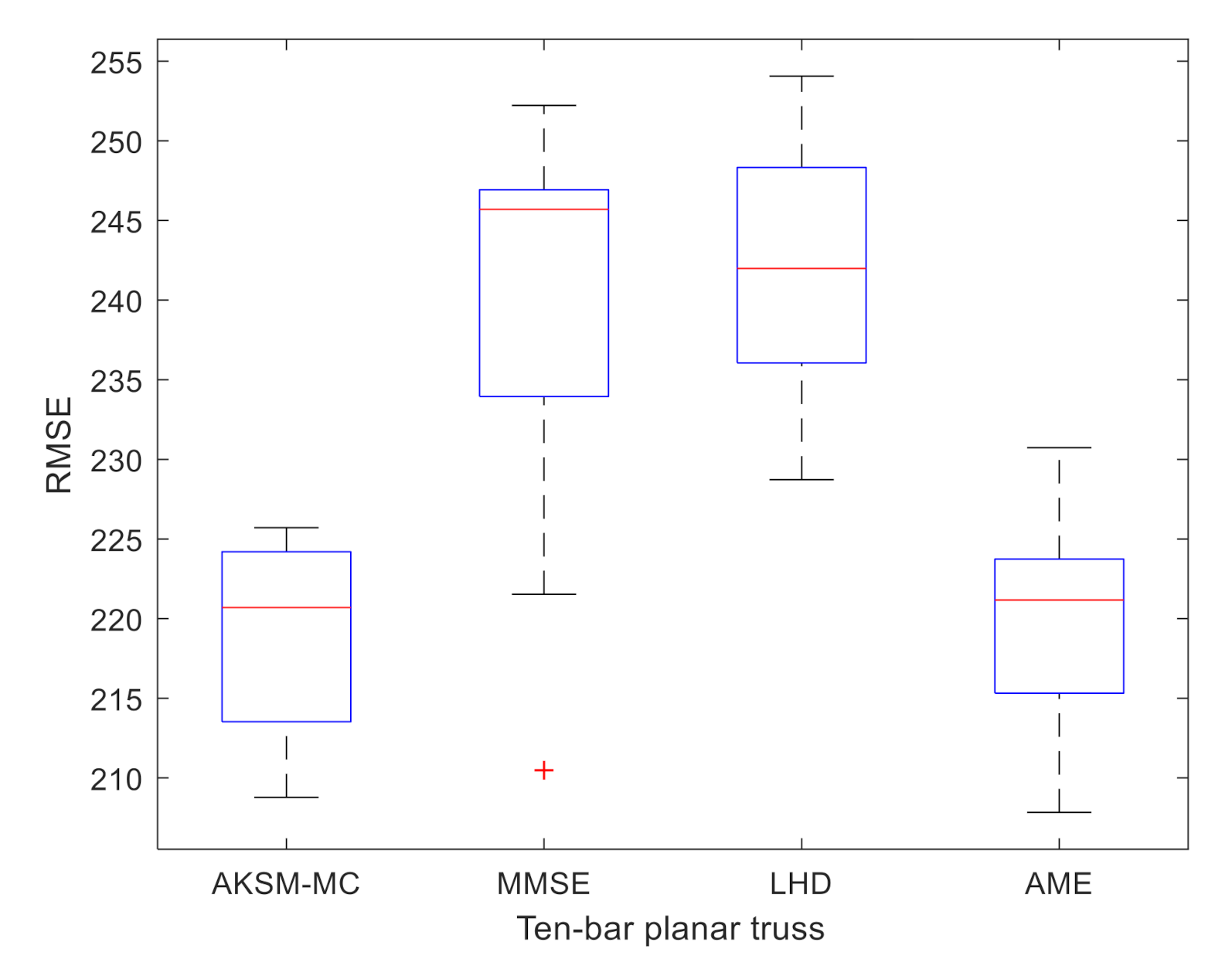
4.2.2. Ten-Bar Planar Truss Problem

Figure 17 is a schematic diagram of a ten-bar planar truss. Barthelemyy was the first to study the ten-bar planar truss [39,40]. The purpose of the study is to minimize the weight of the truss system under the condition that each steel bar stress ${\sigma }_i$ meets the constraint. The ten design variables $x_i\left(i=1,\dots ,10\right)$ are the cross-sectional areas of each steel bar.

The problem is expressed as

$$f(\mathit{x})=36(x_1+x_2+x_3+x_4+x_5+x_6+\sqrt{2}(x_7+x_8+x_9+x_{10}))$$

subject to

$$0.645{\mathrm{cm}}^2\le x_i\le 64.5{\mathrm{cm}}^2\hspace{0.17em}\hspace{0.17em}\hspace{0.17em}\hspace{0.17em}\hspace{0.17em}\hspace{0.17em}i=1,\cdots ,10$$

$$-172375\mathrm{kpa}\le {\sigma }_i\le 172375\mathrm{kpa}\hspace{0.17em}\hspace{0.17em}\hspace{0.17em}\hspace{0.17em}\hspace{0.17em}\hspace{0.17em}i=1,\cdots ,10$$

Table 7. Comparison of modeling results of ten-bar planar truss.

		HKM-HS	MMSE	LHD	AME
RMSE	mean	219.0163	238.4223	241.7911	219.7608
	std	5.8617	12.7105	8.0089	6.5274

shows the RMSE results of 30 runs of each method. Figure 18 is the box plot of RMSE. From Table 7 and Figure 18, it can be seen that compared with AME, MMSE and LHD, the HKM-HS has the smallest average value and standard deviation of RMSE. This shows that the HKM-HS method has the highest modeling accuracy and stability. Therefore, compared with the other three methods, the HKM-HS method is more suitable for solving this problem.

5. House Heating

With the continuous progress of society, the problem of an energy shortage cannot be ignored. Energy conservation has received widespread attention worldwide, and China is no exception. Every winter, house heating is a way to consume energy that cannot be underestimated. In order to reduce energy consumption and reduce pollution to the external environment as much as possible, it is necessary to discuss the issue of house heating [41,42]. There are many factors that affect the heating cost of a house, such as the size of the house, the thermal properties of the house materials, the thermal resistance of the house, the characteristics of the heater, the cost of electricity, and the indoor and outdoor temperatures. Different influencing factors have different degrees of influence on the heating cost of houses. Therefore, predicting the heating cost under different conditions has great practical significance for reducing energy consumption, reducing economic costs and reducing environmental pollution.

Figure 19 is a schematic diagram of house heating. In order to study the relationship between house heating cost and influencing factors, we need to set some influencing factors as variables. Define the length, width and height of the house as variables $x_1$, $x_2$ and $x_3$, respectively. Suppose the number of windows in the house is six and set the length and width of the windows as variables $x_4$ and $x_5$. Set the initial room temperature (outdoor temperature) as variable $x_6$. Set the hot air temperature of the heater as variable $x_7$. Set the thickness of the glass wool on the wall as variable $x_8$. In addition, it is assumed that the flow rate of the heater is $3600\mathrm{kg}/\mathrm{hr}$, the electricity cost is $0.09\$/\mathrm{kWhr}$ and the constant pressure specific heat capacity of air is $1005.4\mathrm{J}/\mathrm{kg}$.

The house heating simulation model was established by MATLAB and SIMULINK. The variables $x_1,\cdots ,x_8$ are used as the input parameters of the simulation, and the heating cost of the house is used as the output variable. The heating cost of the house is related to time. Here we take the day as the unit and the heating cost of the house per day as the output variable. The HKM-HS method was used to determine the new valuation point, that is, to determine the different values of 8 variables (influencing factors), and then estimate the heating cost of a day through simulation. From this, the degree of influence of different influencing factors on heating costs can be explored.

In the process of using the HKM-HS method to achieve house heating, first randomly select 8 initial sample points $x_i(i=1,\cdots ,8)$ through the LHD method and simulate the initial sample points to obtain $y_i(i=1,\cdots ,8)$. Secondly, select new estimation points by the method proposed in this paper and perform simulation until the total number of sample points is 24. In order to ensure the accuracy of the experiment, the average RMSE value of the ten results is taken as the error. RMSE is obtained by the cross-validation method.

Table 8. Comparison of modeling results of house heating.

		HKM-HS	MMSE	LHD	AME
RMSE	mean	0.5738	0.6028	0.6577	0.5866
	std	0.0358	0.0418	0.0338	0.0505

shows the average value and standard deviation of ten RMSE values obtained by applying HKM-HS, MMSE, LHD and AME methods to house heating. The error results show that the modeling accuracy of the HKM-HS method is very good. Figure 20, Figure 21 and Figure 22 is an analysis of the housing heating problem.

Figure 20, Figure 21 and Figure 22 show the relationship between different variables and the heating cost of a house. Through the analysis of the experimental results, we can draw the following conclusions. (1) From Figure 22, the changing trend of $x_6$ and $x_7$ is almost the same as that of the objective value y. This shows that the hot air temperature of the heater and the initial room temperature of the house have a great influence on the heating cost of the house. This may be because the temperature setting of the heater and initial room temperature determine the use time and start-up frequency of the heater. The higher the temperature setting of the heater, the greater the electricity consumption, which will lead to increased electricity cost. On the contrary, the lower the initial room temperature of the house, the higher the electricity cost. (2) In Figure 20, the changing trends of $x_1$, $x_2$, and $x_3$ have some similarities with the changing trends of the objective value y, and the similarity of $x_1$ is more obvious. This indicates that the geometric structure of the house also has a certain influence on the heating cost. The length of the house has the most obvious influence on the heating cost, because the length occupies the largest weight of the house size. The larger the house, the more electricity the heater consumes for heating, and the higher the heating cost. (3) It can be seen in Figure 21 that the changing trends of $x_4$, $x_5$, and $x_8$ are less consistent with that of the objective value y. This implies that these factors have little influence on the heating cost of houses. In short, the HKM-HS method can predict the heating cost of influencing factors under different conditions. Setting a suitable heater temperature according to the size of the house and the initial room temperature can effectively reduce heating cost.

6. Conclusions

The paper proposes a high-precision Kriging modeling method based on hybrid sampling criteria (HKM-HS). First, LHD was used to select the initial sampling point in this method. Secondly, MMSE and MC criteria were optimized to find two candidate points, which were further screened to obtain the final sampling points. Then the HKM-HS modeling method was used to test 16 benchmark functions and three engineering cases. The test results show that the HKM-HS is almost better than other three Kriging-based modeling methods in terms of accuracy and stability. Furthermore, as an actual simulation problem, a housing heating case was used by the proposed method to show that the HKM-HS has a certain degree of engineering application.

However, it is not appropriate for this method to deal with higher dimensional problems. It is the main reason why the increase in dimensions not only causes the construction cost of the Kriging model to rise rapidly, but also cannot guarantee the final modeling accuracy. In view of this, the exploration of high-dimensional problems based on the Kriging model has attracted the attention of some researchers. The key point is how to achieve dimensionality reduction of the high-dimensional Kriging model while ensuring certain accuracy requirements. At present, there are two main ideas to deal with this key issue. One is to transform high-dimensional modeling problems into low-dimensional modeling problems through effective dimensionality reduction methods, thereby increasing the modeling efficiency of Kriging; the other core idea is to reduce the amount of calculation of hyper-parameters in the Kriging modeling process because optimizing hyper-parameters is a very time-consuming task. These research ideas and directions are yet to be further explored and developed by researchers.

References

1. Jensen, W.A. Response surface methodology: Process and product optimization using designed experiments. J. Qual. Technol. 2017, 49, 186. [Google Scholar] [CrossRef]
2. Fan, Y.; Lu, W.; Miao, T.; Li, J.; Lin, J. Multiobjective optimization of the groundwater exploitation layout in coastal areas based on multiple surrogate models. Environ. Sci. Pollut. Res. Int. 2020, 27, 19561–19576. [Google Scholar] [CrossRef] [PubMed]
3. Yan, C.; Shen, X.; Guo, F. An improved support vector regression using least squares method. Struct. Multidiscip. Optim. 2017, 57, 2431–2445. [Google Scholar] [CrossRef]
4. Hamed, Y.; Alzahrani, A.I.; Mustaffa, Z.; Ismail, M.C.; Eng, K.K. Two steps hybrid calibration algorithm of support vector regression and K-nearest neighbors. Alex. Eng. J. 2020, 59, 1181–1190. [Google Scholar] [CrossRef]
5. Fan, C.; Huang, Y.; Wang, Q. Sparsity-promoting polynomial response surface: A new surrogate model for response prediction. Adv. Eng. Softw. 2014, 77, 48–65. [Google Scholar] [CrossRef]
6. Rashki, M.; Azarkish, H.; Rostamian, M.; Bahrpeyma, A. Classification correction of polynomial response surface methods for accurate reliability estimation. Struct. Saf. 2019, 81, 101869. [Google Scholar] [CrossRef]
7. Dou, S.-q.; Li, J.-j.; Kang, F. Health diagnosis of concrete dams using hybrid FWA with RBF-based surrogate model. Water Sci. Eng. 2019, 12, 188–195. [Google Scholar] [CrossRef]
8. Durantin, C.; Rouxel, J.; Désidéri, J.A.; Glière, A. Multifidelity surrogate modeling based on radial basis functions. Struct. Multidiscip. Optim. 2017, 56, 1061–1075. [Google Scholar] [CrossRef] [Green Version]
9. Keshtegar, B.; Mert, C.; Kisi, O. Comparison of four heuristic regression techniques in solar radiation modeling: Kriging method vs RSM, MARS and M5 model tree. Renew. Sustain. Energy Rev. 2018, 81, 330–341. [Google Scholar] [CrossRef]
10. Li, T.; Yang, X. An efficient uniform design for Kriging-based response surface method and its application. Comput. Geotech. 2019, 109, 12–22. [Google Scholar] [CrossRef]
11. van Stein, B.; Wang, H.; Kowalczyk, W.; Emmerich, M.; Bäck, T. Cluster-based Kriging approximation algorithms for complexity reduction. Appl. Intell. 2019, 50, 778–791. [Google Scholar] [CrossRef] [Green Version]
12. Namura, N.; Shimoyama, K.; Obayashi, S. Kriging surrogate model with coordinate transformation based on likelihood and gradient. J. Glob. Optim. 2017, 68, 827–849. [Google Scholar] [CrossRef]
13. Craven, B.A.; Aycock, K.I.; Herbertson, L.H.; Malinauskas, R.A. A CFD-based Kriging surrogate modeling approach for predicting device-specific hemolysis power law coefficients in blood-contacting medical devices. Biomech. Model. Mechanobiol. 2019, 18, 1005–1030. [Google Scholar] [CrossRef] [PubMed]
14. An, X.; Song, B.; Mao, Z.; Ma, C. Layout Optimization Design of Two Vortex Induced Piezoelectric Energy Converters (VIPECs) Using the Combined Kriging Surrogate Model and Particle Swarm Optimization Method. Energies 2018, 11, 2069. [Google Scholar] [CrossRef] [Green Version]
15. Yu, J.; Wang, Z.; Chen, F.; Yu, J.; Wang, C. Kriging surrogate model applied in the mechanism study of tip leakage flow control in turbine cascade by multiple DBD plasma actuators. Aerosp. Sci. Technol. 2019, 85, 216–228. [Google Scholar] [CrossRef]
16. Zeng, F.; Bu, J.; Yu, Y.; Bian, H.; Yang, L.; Zi, X. Optimum design of permanent magnet synchronous generator based on MaxPro sampling and kriging surrogate model. IEEJ Trans. Electr. Electron. Eng. 2020, 15, 278–290. [Google Scholar] [CrossRef]
17. Palar, P.S.; Liem, R.P.; Zuhal, L.R.; Shimoyama, K. On the use of surrogate models in engineering design optimization and exploration: The key issues. In Proceedings of the Genetic and Evolutionary Computation Conference Companion, Prague, Czech Republic, 13–17 July 2019. [Google Scholar]
18. Settles, B. Active Learning Literature Survey; University of Wisconsin-Madison Department of Computer Sciences: Madison, WI, USA, 2009. [Google Scholar]
19. Jin, R.; Chen, W.; Sudjianto, A. On sequential sampling for global metamodeling in engineering design. In Proceedings of the ASME 2002 International Design Engineering Technical Conferences and Computers and Information in Engineering Conference, Montreal, QC, Canada, 29 September–2 October 2002. American Society of Mechanical Engineers Digital Collection. [Google Scholar]
20. Liu, H.; Cai, J.; Ong, Y.-S. An adaptive sampling approach for kriging metamodeling by maximizing expected prediction error. Comput. Chem. Eng. 2017, 106, 171–182. [Google Scholar] [CrossRef]
21. Liu, H.; Xu, S.; Ma, Y.; Chen, X.; Wang, X. An Adaptive Bayesian Sequential Sampling Approach for Global Metamodeling. J. Mech. Des. 2016, 138, 011404. [Google Scholar] [CrossRef]
22. Sacks, J.; Welch, W.J.; Mitchell, T.J.; Wynn, H.P. Design and analysis of computer experiments. Stat. Sci. 1989, 4, 409–423. [Google Scholar] [CrossRef]
23. Jiang, P.; Zhang, Y.; Zhou, Q.; Shao, X.; Hu, J.; Shu, L. An adaptive sampling strategy for Kriging metamodel based on Delaunay triangulation and TOPSIS. Appl. Intell. 2018, 48, 1644–1656. [Google Scholar] [CrossRef]
24. Xu, J.; Dang, C. A novel fractional moments-based maximum entropy method for high-dimensional reliability analysis. Appl. Math. Model. 2019, 75, 749–768. [Google Scholar] [CrossRef]
25. Zeng, W.; Sun, W.; Song, H.; Ren, T.; Sun, Y. A parallel adaptive sampling strategy to accelerate the sampling process during the modeling of a Kriging metamodel. J. Chin. Inst. Eng. 2019, 42, 676–689. [Google Scholar] [CrossRef]
26. Wei, X.; Wu, Y.-Z.; Chen, L.-P. A new sequential optimal sampling method for radial basis functions. Appl. Math. Comput. 2012, 218, 9635–9646. [Google Scholar] [CrossRef]
27. Cai, X.; Qiu, H.; Gao, L.; Yang, P.; Shao, X. A multi-point sampling method based on kriging for global optimization. Struct. Multidiscip. Optim. 2017, 56, 71–88. [Google Scholar] [CrossRef]
28. Li, Y. A Kriging-based multi-point sequential sampling optimization method for complex black-box problem. Evol. Intell. 2020, 1–10. [Google Scholar] [CrossRef]
29. Liu, B.; Xie, L. An Improved Structural Reliability Analysis Method Based on Local Approximation and Parallelization. Mathematics 2020, 8, 209. [Google Scholar] [CrossRef] [Green Version]
30. Nielsen, H.B. Aspects of the Matlab Toolbox DACE; Technical University of Denmark: Kongens Lyngby, Denmark, 2002. [Google Scholar]
31. Lophaven, S.; Nielsen, H.; Sondergaard, J.; Dace, A. A Matlab Kriging Toolbox; Technical Report, No. IMMTR-2002-12; Technical University of Denmark: Kongens Lyngby, Denmark, 2002. [Google Scholar]
32. Rasmussen, C.E.; Williams, C.K.I. Gaussian Processes for Machine Learning; The MIT Press: Cambridge, MA, USA, 2005. [Google Scholar]
33. Palar, P.S.; Shimoyama, K. Efficient global optimization with ensemble and selection of kernel functions for engineering design. Struct. Multidiscip. Optim. 2018, 59, 93–116. [Google Scholar] [CrossRef]
34. Yuan, G.L.; Yu, T.; Du, J. Multi-Objective Optimal Load Distribution Based on Sub Goals Multiplication and Division in Power Plants. Appl. Mech. Mater. 2014, 494–495, 1715–1718. [Google Scholar] [CrossRef]
35. Yun, Y.; Chuluunsukh, A.; Gen, M. Sustainable Closed-Loop Supply Chain Design Problem: A Hybrid Genetic Algorithm Approach. Mathematics 2020, 8, 84. [Google Scholar] [CrossRef] [Green Version]
36. Schobi, R.; Sudret, B.; Wiart, J. Polynomial-chaos-based kriging. Int. J. Uncertain. Quantif. 2015, 5, 171–193. [Google Scholar] [CrossRef]
37. Xiong, Y.; Chen, W.; Apley, D.; Ding, X. A non-stationary covariance-based Kriging method for metamodelling in engineering design. Int. J. Numer. Methods Eng. 2010, 71, 733–756. [Google Scholar] [CrossRef]
38. Arora, J.S. Optimum Design with Excel Solver. In Introduction to Optimum Design; Academic Press: Cambridge, MA, USA, 2012; pp. 213–273. [Google Scholar]
39. Sobieszczanski-Sobieski, J.; Barthelemy, J.-F.; Riley, K.M. Sensitivity of Optimum Solutions of Problem Parameters. AIAA J. 1982, 20, 1291–1299. [Google Scholar] [CrossRef] [Green Version]
40. Schmit, L.A.; Farshi, B. Some Approximation Concepts for Structural Synthesis. AIAA J. 1974, 12, 692–699. [Google Scholar] [CrossRef]
41. Fan, Y.; Zhao, X.; Li, J.; Li, G.; Myers, S.; Cheng, Y.; Badiei, A.; Yu, M.; Akhlaghi, Y.G.; Shittu, S.; et al. Economic and environmental analysis of a novel rural house heating and cooling system using a solar-assisted vapour injection heat pump. Appl. Energy 2020, 275, 115323. [Google Scholar] [CrossRef]
42. Bezyan, B.; Zmeureanu, R. Machine Learning for Benchmarking Models of Heating Energy Demand of Houses in Northern Canada. Energies 2020, 13, 1158. [Google Scholar] [CrossRef] [Green Version]
Figure 1. (a) Kriging approximate function based on different correlation functions; (b) absolute error (AE) of Kriging approximation functions.
Mathematics 09 00536 g001
Figure 2. (a) AE of Kriging approximation functions in the three-dimensional question; (b) AE of Kriging approximation functions in the five-dimensional question.
Mathematics 09 00536 g002
Figure 3. The flowchart of the HKM-HS method.
Mathematics 09 00536 g003
Figure 4. (a)Test result of Bukin function by HKM-HS; (b) Test result of Bukin function by maximum mean square error (MMSE); (c) Test result of Bukin function by Latin Hypercube Design (LHD); (d) Test result of Bukin function by adaptive maximum entropy (AME).
Mathematics 09 00536 g004
Figure 5. (a)Test result of Schwefel function by HKM-HS; (b) Test result of Schwefel function by maximum mean square error (MMSE); (c) Test result of Schwefel function by Latin Hypercube Design (LHD); (d) Test result of Schwefel function by adaptive maximum entropy (AME).
Mathematics 09 00536 g005
Figure 6. (a)Test result of Mccormick function by HKM-HS; (b) Test result of Mccormick function by maximum mean square error (MMSE); (c) Test result of Mccormick function by Latin Hypercube Design (LHD); (d) Test result of Mccormick function by adaptive maximum entropy (AME).
Mathematics 09 00536 g006
Figure 7. (a)Test result of sixHump function by HKM-HS; (b) Test result of sixHump function by maximum mean square error (MMSE); (c) Test result of sixHump function by Latin Hypercube Design (LHD); (d) Test result of sixHump function by adaptive maximum entropy (AME).
Mathematics 09 00536 g007
Figure 8. (a)Test result of Alpine function by HKM-HS; (b) Test result of Alpine function by maximum mean square error (MMSE); (c) Test result of Alpine function by Latin Hypercube Design (LHD); (d) Test result of Alpine function by adaptive maximum entropy (AME).
Mathematics 09 00536 g008
Figure 9. (a)Test result of Gp function by HKM-HS; (b) Test result of Gp function by maximum mean square error (MMSE); (c) Test result of Gp function by Latin Hypercube Design (LHD); (d) Test result of Gp function by adaptive maximum entropy (AME).
Mathematics 09 00536 g009
Figure 10. (a) Box plot of test results for Levy function; (b) Box plot of test results for Rastrigin function.
Mathematics 09 00536 g010
Figure 11. (a) Box plot of test results for DixonPrice function; (b) Box plot of test results for Rosenbrock function.
Mathematics 09 00536 g011
Figure 12. (a) Box plot of test results for Michalewicz function; (b) Box plot of test results for Michalewice10 function.
Mathematics 09 00536 g012
Figure 13. (a) Box plot of test results for Hartman3 function; (b) Box plot of test results for Shekel function.
Mathematics 09 00536 g013
Figure 14. (a) Box plot of test results for Hartman6 function; (b) Box plot of test results for F16 function.
Mathematics 09 00536 g014
Figure 15. Spring design.
Mathematics 09 00536 g015
Figure 16. Box plot of the RMSE values of the four methods.
Mathematics 09 00536 g016
Figure 17. Ten-bar planar truss.
Mathematics 09 00536 g017
Figure 18. Box plot of the RMSE values of the four methods.
Mathematics 09 00536 g018
Figure 19. House heating.
Mathematics 09 00536 g019
Figure 20. Trends of design variables x 1 , x 2 , x 3 and objective function obtained by HKM-HS.
Mathematics 09 00536 g020
Figure 21. Trends of design variables x 4 , x 5 , x 8 and objective function obtained by HKM-HS.
Mathematics 09 00536 g021
Figure 22. Trends of design variables x 6 , x 7 and objective function obtained by HKM-HS.
Mathematics 09 00536 g022