Abstract
We consider the problem of scheduling n jobs with identical processing times and given release as well as delivery times on m uniform machines. The goal is to minimize the makespan, i.e., the maximum full completion time of any job. This problem is well-known to have an open complexity status even if the number of jobs is fixed. We present a polynomial-time algorithm for the problem which is based on the earlier introduced algorithmic framework blesscmore (“branch less and cut more”). We extend the analysis of the so-called behavior alternatives developed earlier for the version of the problem with identical parallel machines and show how the earlier used technique for identical machines can be extended to the uniform machine environment if a special condition on the job parameters is imposed. The time complexity of the proposed algorithm is , where can be either n or the maximum job delivery time . This complexity can even be reduced further by using a smaller number in the estimation describing the number of jobs of particular types. However, this number becomes only known when the algorithm has terminated.
1. Introduction
In this paper, we consider a basic optimization problem of scheduling jobs with release and delivery times on uniform machines with the objective to minimize the makespan. More precisely, n jobs from the set are to be processed by m parallel uniform machines (or processors) from the set . Job is available from its release time; it needs a continuous (integer) processing time p, which is the time that it needs on a slowest machine. We assume that the machines in the set M are ordered by their speeds, the fastest machines first, i.e., are the corresponding machine speeds, being the speed of machine i. Without loss of generality, we assume that , and the processing time of job j on machine i is an integer . Job j has one more parameter, the delivery time , an integer number which represents the amount of additional time units which are necessary for the full completion of job j after it completes on the machine. Thus, notice that the delivery of job j consumes no machine time (the delivery is accomplished by an independent agent).
Now, we define a feasible schedule S as a function that assigns to each job j a starting time and a machine i from the set M such that, for any job j, we have and holds for any job k scheduled before job j on the same machine. Note that the first inequality requires that a job cannot start its processing before before the given release time, and the second one describes the constraint that each machine can process only one job at any time. The completion time of job j in the schedule S is the time moment when the processing of job i is complete on the machine i to which it is assigned in the schedule S, i.e., and the full completion time of job j in the schedule S is (the full completion time of job j takes into account the delivery time of that job, whereas the completion time of job j does not depend on its delivery time). The goal is to determine an optimal schedule S being feasible and minimizing the maximum full job completion time of any job
or the makespan.
The studied multiprocessor optimization problem, described below, is commonly abbreviated as (its version with identical parallel machines is abbreviated as , the first field specifies the machine environment, the second one the job parameters, and the third one the objective function).
It is well-known that there is an equivalent (perhaps more traditional) formulation of the above described problem, in which, instead of the delivery time , every job j has its due-date . The lateness of job j in the schedule S is . Then, the objective becomes to minimize the maximum job lateness , i.e., find a feasible schedule in which the maximum job lateness is not more than in any other feasible schedule, i.e., is an optimal schedule. The equivalence is easily established by associating with each job delivery time a corresponding due-date, and, vice-versa, see e.g., Bratley et al. [1]). The version of the problem with due-dates with identical and uniform machine environments are commonly abbreviated as and , respectively.
For the problem considered, each machine from a group of parallel uniform machines is characterized by its own speed, independent from a particular job that can be assigned to it, unlike a machine from a group of unrelated machines whose speed is job-dependent. Because of the uniform speed characteristic, scheduling problems with uniform machines are essentially easier than scheduling problems with unrelated machines, whereas scheduling problems with identical machines are easier than those with uniform ones.
The general problem of scheduling jobs with release and delivery times on uniform machines is well-known to be strongly NP-hard as already the single-machine version is strongly NP-hard. However, if all jobs have equal processing times, the problem can be polynomially solved on identical machines. The version on uniform machines is a long-standing open problem even in case the number of machines m is fixed. In this paper, we present a polynomial-time algorithm for the uniform machine environment which finds an optimal solution to the problem if for any pair of jobs i and j with and , we have
The proposed algorithm relies on the blesscmore (“branch less, cut more”) framework for the identical machine case from [2] (the blesscmore algorithmic concept was formally introduced later in [3]). A blesscmore algorithm generates a solution tree similar to a branch-and-bound algorithm, however, the branching and cutting criteria are based on a direct analysis of some structural properties of the problem under consideration without using lower bounds. The algorithmic framework, on which the blesscmore algorithm that we describe here is based, takes an advantage of some nice structural properties of specially created schedules which are analyzed in terms of the so-called behavior alternatives from [2]. The framework resulted in an time algorithm with being the maximum delivery time of a job and being a parameter which becomes known only after the algorithm has terminated. Each schedule is easily created by a well-known greedy algorithm commonly referred to as Largest Delivery Time heuristic (LDT-heuristic for short): iteratively, among all released jobs, it schedules one with the largest delivery time. The algorithm from [2] carries out the enumeration of LDT-schedules (ones created by the LDT-heuristic)—it is known that there is an optimal LDT-schedule. Based on the established properties, the set of LDT-schedules is reduced to a subset of polynomial size which yields a polynomial time overall performance. Although the LDT-heuristic applied to a problem instance with uniform machines does not provide the desirable properties, it can be modified to a similar method that takes into account the uniform speed characteristic. While scheduling identical machines, the minimum completion time of each next selected job is always achieved on the machine next to the one to which the previous job was assigned. With uniform machines, this is not necessarily the case, for example, the next machine can be much slower than the current one. Hence, the time moment at which the job will complete on each of the machines needs to be additionally determined and then this job can be assigned to a machine on which the above minimum is reached. In this paper, we use an adaptation of the LDT-heuristic, which will be referred to as the LDTC-heuristic, and a schedule created by the later heuristic will be referred to as an LDTC-schedule. Instead of enumerating the LDT-schedules (as in [2]), the algorithm proposed here enumerates LDTC-schedules. Some properties for the identical machine environment which do not immediately hold for uniform machines are reformulated in terms of uniform machines, which allows for maintaining the basic framework from [2], which, as suggested earlier, turned out to be sufficiently flexible.
Similarly to the existence of an optimal LDT-schedule for the identical machine environment, there exists an optimal LDTC-schedule for the uniform machine environment. The complete enumeration of the LDTC-schedules is avoided by the generalization of nice properties of LDT-schedules to LDTC-schedules for uniform machines. These properties are obtained via the analysis of the so-called behavior alternatives from [2] that are generalized for uniform machines. The algorithm presented in this paper in the worst case requires steps with being any of the number n of jobs or the maximum delivery time of a job. In fact, n can be replaced by a smaller magnitude , the number of special types of jobs; this is the same parameter as for the algorithm from [2], which becomes known only when the algorithm halts. The running time of the proposed algorithm is worse than that of the one from [2], in part because of the cost of the LDTC-heuristic which is repeatedly used during the solution process.
The remainder of this paper is as follows: in Section 2, we give a brief literature review. Section 3 presents some necessary preliminaries. Then, the basic algorithmic framework is given in Section 4. Section 5 discusses the performance analysis of the developed blesscmore algorithm. Section 6 contains a final discussion and concluding remarks.
2. Literature Review
If the job processing times are arbitrary, then the problem is known to be strongly NP-hard, even if there is only a single machine [4]. McMahon & Florian [5] gave an efficient branch and bound algorithm, and Carlier [6] later adopted it for the version with jobs delivery times (a solution to the latter version can immediately be used for the calculation of lower bounds for a more general job shop scheduling problem). For the single machine case, Baptiste gave an algorithm for the problem [7] and also an algorithm of the same complexity for the problem [8] of minimizing the weighted number of late jobs. Chrobak et al. [9] have derived an algorithm of improved complexity for the case of unit weights, i.e., for the problem . Later, Vakhania [10] gave an blesscmore algorithm for this problem. Note that, for the problem with arbitrary processing times and allowed preemptions, Vakhania [11] derived an blesscmore algorithm.
One may consider a slight relaxation of problems , and in which one looks for a schedule in which no job completes after its due-date. Such a feasibility setting with a single machine was considered by Garey et al. [12]. They have proposed an algorithm that has further been improved to an one by using a very sophisticated data structure. This paper uses the concept of a so-called forbidden region describing an interval in which it is forbidden to start any job in a feasible schedule. Later, Simons and Warmuth [13] have constructed an time algorithm for the feasibility setting with the identical machine environment also using the concept of forbidden regions. (It can be mentioned that the minimization version of the problem can be solved by applying an algorithm for the feasibility problem by repeatedly increasing the due-dates of all jobs until a feasible schedule with the modified due dates is found. Using binary search makes such a reduction procedure more efficient and reduces the reduction cost to .)
Dessousky et al. [14] considered scheduling problems on uniform machines with simultaneously released jobs (i.e., with for every job j) and with different objective criteria. They proposed fast polynomial-time algorithms for these problems, in particular, for the criterion . In fact, the LDTC-heuristic is an adaptation of an optimal solution method that the authors in [14] constructed for the criterion .
For a uniform machine environment with allowed preemptions (), the problem is polynomially solvable even for arbitrary processing times [15], while a polynomial algorithm for the problem with minimizing total weighted completion time in the case of equal processing times has been given in [16]. The case of unrelated machines is very hard. A polynomial algorithm exists for the problem with allowed preemptions and minimizing maximum lateness, even for the case of arbitrary processing times [17]. If preemptions are forbidden, Vakhania et al. [18] gave a polynomial algorithm for the case of minimizing the makespan when only two processing times p and are possible (i.e., for the problem . Note that the case of two arbitrary processing times p and q is known to be NP-hard [19]. For the special case of identical parallel machines, there exist several works for the same setting as considered in this paper but for more complicated objective functions regarding the complexity status. In particular, the problems of minimizing the weighted sum of completion times [20] and of minimizing total tardiness [21] can be polynomially solved by a reduction to a linear programming problem. In [3], Vakhania presented an blesscmore algorithm for the problem of minimizing the number of late jobs. His blesscmore algorithm uses a solution tree, where the branching and cutting criteria are based on the analysis of behavior alternatives. Moreover, the problem can also be polynomially solved for the case that is an arbitrary non-decreasing function such that the difference is monotonic for any indices i and j [22]. The authors also applied a linear programming approach. An overview of selected solution approaches for some related scheduling problems with equal processing times is given in Table 1. It can also be mentioned that a detailed survey on parallel machine scheduling problems with equal processing times has been given in [23].

Table 1.
Overview of solution approaches for related problems with equal processing times.
3. Preliminaries
This section contains some useful properties, necessary terminology, and concepts, some of which were introduced in [2] for identical machines.
LDTC-heuristic. We first describe the LDTC-heuristic, an adaptation of the LDT-heuristic for uniform machines. As earlier briefly noted, unlike an LDT-schedule, an LDTC-schedule is not defined by a mere permutation of the given n jobs since the machine to which the next selected job is assigned depends on the machine speed. Starting from the minimal job release time, the current scheduling time is iteratively set as the minimum release time among all yet unscheduled jobs. Iteratively, among all jobs released by the current scheduling time, the LDTC-heuristic determines one with the largest delivery time (a most urgent one) and schedules it on the machine on which the earliest possible completion time of this job is attained (ties can be broken by selecting the machine with the minimum index):
Note that, in an LDTC-schedule S, a machine will contain an idle-time interval (a gap) if and only if there is no unscheduled job released by the current scheduling time. The running time of the modified heuristic is the same as that of the LDT-heuristic with an additional factor of m due to the machine selection at each iteration (which is not required for the uniform machine environment), which results in the time complexity .
Example 1.
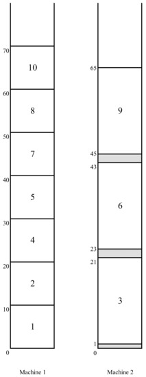
We shall illustrate the basic notions and the algorithm described here on a small problem instance with 10 jobs and two uniform machines with and . The processing time of all jobs (on machine 2) is 20. The rest of the parameters of these jobs are defined as follows: , , and . , , and . The LDTC-schedule obtained by the LDTC-heuristic for the problem instance of the above example is depicted in Figure 1. In general, we denote the LDTC-schedule obtained by the LDTC-heuristic for the initially given instance of problem by σ (as we will see in the following subsection, we may generate alternative LDTC-schedules by iteratively modifying the originally given problem instance).
Figure 1.
Initial LDTC schedule .
The next property of an LDTC-schedule easily follows from the definition of the LDTC-heuristic and the equality of the job processing times (job j is said to have the ordinal number i in schedule S if it is the ith scheduled job in that schedule S):
Property 1.
If in an LDTC-schedule S, job j is scheduled after job i, i.e., the ordinal number of job j in S is larger than that of job i, then .
Next, we give another easily seen important property of an LDTC-schedule S on which the proposed method essentially relies. Let A be a set of, say k jobs, all of which being released by time moment t, and let be any permutation of k jobs all of them being also released by time t (recall that all the jobs have equal length). Let, further, be a partial LDTC-schedule constructed for the jobs in the set A, and let be a list schedule constructed for the permutation (it includes the jobs according to the order in permutation , leaves no avoidable gap, and assigns each job to the machine on which it will complete sooner breaking ties again by selecting the machine with the minimum index). The following property, roughly, states that both above schedules are indistinguishable if the delivery times of the jobs are ignored:
Property 2.
The completion time of every machine in both schedules and is the same. Moreover, the ith scheduled job in the schedule starts and completes at the same time as the ith scheduled job on the corresponding machine in the schedule .
The above property also holds for a group of identical machines and is helpful for the generalization of the earlier results for identical machines from [2] to uniform machines. Roughly, ignoring the job release times, the property states that two list schedules constructed for two different permutations with the same number of jobs have the same structure. Although the starting and completion times of the jobs scheduled in the same position on the corresponding machine are the same in both schedules, the full completion times will not necessarily be the same (this obviously depends on the delivery times of these jobs).
A block. A consecutive independent part in a schedule is commonly referred to as a block in the scheduling literature. We define a block in an LDTC-schedule S as the largest fragment (a consecutive sequence of jobs) of that schedule such that, for each two successively scheduled jobs i and j, job j starts no later than job i finishes (jobs i and j can be scheduled on the same or different machines according to the LDTC-heuristic). It follows that there is a single block that starts schedule S and there is also a single block that finishes this schedule. If these blocks coincide, then there is a single block in the schedule S; otherwise, each next block is “separated” from the previous one with gaps on each of the machines. Here, a zero length gap between jobs i and j will be distinguished in case job j is scheduled at time on the same machine as job i (it immediately succeeds job i on this machine). It is easily observed that the schedule given in Figure 1 consists of a single block (note that the order in which the jobs are included in this schedule coincides with the enumeration of these jobs).
A block B (with at least two elements) possesses the following property that will be used later. Suppose the th scheduled job j (not the last scheduled job of the block) is removed from that block and the LDTC-heuristic is applied to the remaining jobs of the block. As a consequence, in the resulting (partial) schedule, the processing interval of the job scheduled as the th one overlaps with the processing interval of job j in the block B earlier.
Some additional definitions are required to specify how the proposed algorithm creates and evaluates the feasible schedules. At any stage of the execution of the algorithm, independently whether a new LDTC-schedule will be generated or not, depends on specific properties of the LDTC-schedules already generated by that stage. The definitions below are helpful for the determination of these properties.
An overflow job. In an LDTC-schedule S, let o be a job realizing the maximum full completion time of a job, i.e.,
and let be the critical block in the schedule S, i.e., the block containing the earliest scheduled job o satisfying Equation (2). The overflow job in the schedule S is the last scheduled job in the block satisfying Condition (2), i.e., one with the maximum . It can be easily verified that in the schedule in Figure 1, job 7 is the overflow job with (the full completion time of the latest completed job 10 is ).
A kernel. Next, we define an important component in an LDTC-schedule S defined as its fragment containing the overflow job such that the jobs scheduled before job o in the block have a delivery time not smaller than (we will write o instead of when this causes no confusion). This sub-fragment of the block is called its kernel and is denoted by . The kernel in the schedule in Figure 1 is the fragment of that schedule constituted by the jobs 5, 6, and 7.
Intuitively, on the one hand, the kernel is a critical part in a schedule S, and, on the other hand, it is relatively easy to arrange the kernel jobs optimally. In fact, we will explore different LDTC-schedules identifying the kernel in each of these schedules. We will also relate this kernel to the kernels of the earlier generated LDTC-schedules. We need to introduce a few more definitions.
An emerging job. Suppose that a job j of kernel is pushed by a non-kernel job e scheduled before that job in the block , that is, the LDTC-heuristic would schedule job j earlier if job i was forced to be scheduled after job j. If , then job e is called a regular emerging job in the schedule S, and the latest scheduled (regular) emerging job (the one closest to job o) is called the delaying emerging job. The emerging jobs in the schedule in Figure 1 are jobs 1, 2, 3, and 4, and job 4 is the delaying emerging job (in general, there may exist a non-kernel non-emerging job scheduled before the kernel in the block ).
The following optimality condition can be established already in the initial LDTC-schedule .
Lemma 1.
If the initial LDTC-schedule σ contains a kernel K such that no job of that kernel is pushed by an emerging job, then this schedule is optimal.
Proof.
Using an interchange argument, we show that no reordering of the jobs of the kernel K can be beneficial. First, we note that the first job j of kernel K must be scheduled on machine 1 since otherwise, it would have been pushed by the corresponding job scheduled on that machine. But this job cannot exist since, by the condition of the lemma, it cannot be pushed by an emerging job (and if it is not an emerging job, it should have been a part of kernel K). Since machine 1 will finish job j at least as early as any other machine, the full completion of job j cannot be reduced.
Let i and j be two successively scheduled jobs from the kernel K, and be the machines to which jobs i and j are assigned, respectively, in the schedule . Without loss of generality, assume that as otherwise it is easy to see that interchanging jobs i and j cannot give any benefit. We let be the schedule obtained from schedule by interchanging jobs i and j.
Assume first that jobs i and j are among the first m (or less) scheduled jobs from the kernel K. By the condition of the lemma, both jobs start at their release time in the schedule . We show that interchanging jobs i and j cannot be beneficial by establishing that
Since , , hence we need to show that . Since , it will suffice to show that
We have
and
However, by Condition (1), , which establishes Inequality (3).
Suppose now that jobs i and j are not among the first m scheduled jobs of the kernel K. If by the current scheduling time both jobs are released, then by a similar interchange argument Inequality (3) can easily be established (without using Condition (1)).
It remains to consider the case when job j is released within the execution interval of job i, hence . We have
Again, by Condition (1), and Inequality (3) again holds.
Applying repeatedly the above interchange argument to all pairs of jobs from the kernel K, we obtain that no rearrangement of the jobs of kernel K may result in a maximum full job completion time less than that of the overflow job , i.e., the schedule is optimal. □
Constructing Alternative LDTC-Schedules
Due to Lemma 1, from here on, it is assumed that the condition in this lemma is not satisfied, i.e., there exists an emerging job e in the schedule S (note that as otherwise job e may not push a job of the kernel ). Since job e is pushing a job of kernel , the removal of this job may potentially decrease the start and hence the full completion time of the overflow job . At the same time, note again that, by the definition of a block, the omission of a job not from the block may not affect the starting time of any job from the block . This is why we restrict here our attention to the jobs of the block . (Here, we only mention that later we will also apply an alternative notion of a passive emerging job, and then the notion “emerging job” is used either for a regular or a passive emerging job; until then, we use “emerging job” for a “regular emerging job”).
Clearly, no emerging job can actually be removed as the resultant schedule would be infeasible. Instead, to restart the jobs in the kernel earlier, an emerging job e is applied to this kernel, i.e., it is forced to be rescheduled after all jobs of the kernel whereas any job, scheduled after the kernel in the schedule S, is maintained to be scheduled after that kernel. The LDTC-heuristic is newly applied with the restriction that the scheduling of job e and all jobs, scheduled after kernel in schedule S is forbidden until all jobs of kernel are scheduled. The resultant LDTC-schedule is denoted by (the so-called complementary schedule or a C-schedule) (Such a schedule generation technique was originally suggested by McMahon and Florian [5] for the single-machine setting.)
By Lemma 1, the kernel , a fragment of the LDTC-schedule S considered as an independent LDTC-schedule is optimal if it possesses no emerging job. Otherwise, the jobs of the kernel are pushed by the corresponding emerging jobs. Some of these emerging jobs can be scheduled after the kernel in an optimal complete schedule . Such a rescheduling is achieved by the creation of the corresponding C-schedules (as we will see in Lemma 2, it will suffice to consider only C-schedules, i.e., is a C-schedule). In Figure 2, a complementary schedule is depicted in which the delaying emerging job 4 is rescheduled after all jobs of kernel (where is the initial LDTC-schedule of Figure 1).
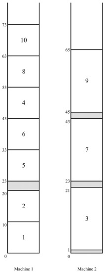
Figure 2.
The C-schedule .
The application of an emerging job has two “opposite” effects. On the positive side, since the number of jobs scheduled before the kernel in the schedule is one less than that in the schedule S, the overflow job in the schedule will be completed earlier than it was completed in the schedule S; likewise, the completion time of that job, which is scheduled as the latest one of the kernel in the schedule , will be smaller than the completion time of the job in the schedule S. Hence, the application of an emerging job gives a potential to improve schedule S. On the negative side, it creates a new gap within the former execution interval of job e or at a later time moment before kernel (see Lemma 1 in [2] for a proof for the case of identical machines, the uniform machine case can be proved similarly). Such a gap may enforce a right-shift (delay) of the jobs included after job e in the schedule ; (for example, a new gap “[20–23]” that arises for machine 1 in the C-schedule in Figure 2 enforces a right-shift of jobs 8 and 10 included behind job 4). Thus, roughly, the C-schedule favors the kernel but creates a potential conflict for later scheduled jobs (jobs 8 and 10 in the above example).
4. The Basic Algorithmic Framework
In this section, we give the basic skeleton of the algorithm in this paper and prove its correctness. The schedule is characterized by a proper processing order of the emerging jobs scheduled in between the kernels. Starting with the initial LDTC-schedule , an emerging job in the current LDTC-schedule is applied and a new C-schedule is created; in this schedule, the kernel is again determined. The same operation is iteratively repeated as long as the established optimality conditions are not satisfied. As we will show later, it will suffice to enumerate all C-schedules to find an optimal solution to the problem.
We associate a complete feasible C-schedule with each node in a solution tree T, the initial LDTC-schedule being associated with the root. Aiming to avoid a brutal enumeration of all C-schedules, we carry out a deeper study of the structure of the problem and some additional useful properties of LDTC-schedules. In fact, our solution tree T consists of a single chain of C-schedules. We will refer to a node of the tree as a stage (since each node represents a particular stage in the algorithm with the corresponding LDTC-schedule). We let be the sequence of C-schedules generated by stage h. Thus, is the initial LDTC-schedule, and the schedule of stage , the immediate successor of schedule , is obtained by one of the extension rules as described below.
In the schedule , the overflow job , the delaying emerging job l, and the kernel are determined. Using the normal extension rule, we let , where l is the delaying emerging job in the schedule (we may observe that the schedule in Figure 2 is obtained from the schedule by the normal extension rule). Alternatively, the schedule is constructed from the schedule by the emergency extension rule as described in the following subsection.
4.1. Types of Emerging Jobs and the Extended Behavior Alternatives
A marched emerging job. An emerging job may be in different possible states. It is useful to distinguish these states and treat them accordingly. Suppose that e is an emerging job in the schedule , and it is applied by stage h, (in a predecessor-schedule of schedule ). Then, job e is called marched in the schedule if (job 4 is marched in the schedule in Figure 2). Intuitively, the existence of a marched job in the schedule indicates an “interference” of the kernel with an earlier arranged part of the schedule preceding that kernel. In our example, it is easy to see that the kernel consists of jobs 8, 9, and 10, with and with . Here, the marched job 4 has “provoked” the rise of the new kernel, where “the earlier arranged part” includes the kernel of the initial LDTC-schedule in Figure 1.
A stuck emerging job. Suppose that job e is marched in the schedule and , where is a non-primary block. Then, job e is called stuck in the schedule if either it is scheduled before job or (observe that any job stuck in the schedule belongs to the kernel ). In Figure 3, the C-schedule obtained from the C-schedule by the application of the delaying emerging job 4 is depicted. Job 4 becomes the overflow job in the schedule (with ) and, hence, it is stuck in this schedule.
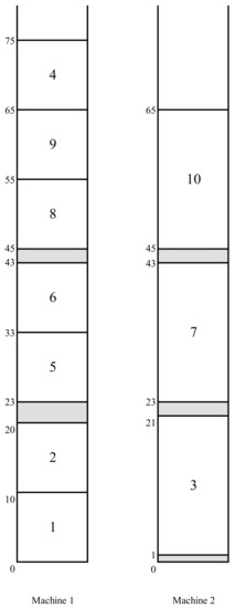
Figure 3.
The C-schedule .
Block evolution in the solution treeT. Although , since is a non-primary block, a “potential” regular emerging job might be “hidden” in some block preceding block , in the schedule . In general, a block in the schedule can be a part of a larger block from the schedule for some . Recall that the application of an emerging job e in a C-schedule S yields the raise of a new gap in the C-schedule . As it can be straightforwardly seen, this can lead to a separation or to a splitting of the critical block into two (or possibly even more) new blocks. Likewise, since job e may push the following jobs in the schedule because of the forced right-shift of these jobs, two or more blocks may merge forming a bigger block consisting of the jobs from the former blocks.
We will refer to blocks from two different C-schedules as congruent if both of them are formed by the same set of jobs. A block in a C-schedule, which is congruent to a block from the initial LDTC-schedule, will be referred to as a primary block. Observe that a non-primary block may arise because of either block splitting or/and block merging and that all blocks in the initial LDTC-schedule are primary.
If the block B arises as a result of an application of an emerging job e, then this block is said to be a non-primary block of job e, and the latter job is said to be the splitting job of B. Note that, since the application of an emerging job does not necessarily lead to a splitting of a block, a non-primary block of job e may contain some other emerging jobs which have already been applied (recall that, before each application of an emerging job, the current release time of this job has to be increased accordingly; e.g., if job e is applied times, its release time is modified times).
In the following, we call the blocks which arose after the splitting of one particular block as the direct descendants of this block (the latter block is called the direct predecessor of the former ones). Moreover, if the block is the direct predecessor of the blocks , then the inclusion holds, but not the opposite one (due to a possible merging of blocks).
Recurrently, a descendant of a block is its direct descendant, since any descendant of a descendant of a block is obviously also a descendant of the latter block. Moreover, if a block is a descendant of another block, then the latter one is called a predecessor of the former block. Subsequently, we call two or more blocks relative if they possess at least one common predecessor block.
Returning to our example, the primary block from the schedule in Figure 1 is split into its two direct descendant blocks with the jobs 1, 2, 3 and 5, 6, 7, 4, 8, 9, 10, respectively, in the schedule in Figure 2. The splitting job is the marched job 4. The first block in the schedule is congruent to the first block in the schedule in Figure 3. The second block in the schedule is further split into two blocks in the schedule , and the splitting job is again job 4. The third block in the schedule (consisting of the jobs 8, 9, 10, and 4 is a descendant of the primary block in the schedule .
A passive emerging job. A passive emerging job e in the schedule is a (“hidden”) regular emerging job from the schedule , i.e., job e belongs to a block from the schedule , relative to block (preceding this block), such that . For example, in the schedule in Figure 2, the passive emerging jobs are 1, 2, and 3, and in the schedule in Figure 3, the passive emerging jobs are 1 and 2.
Extended behavior alternatives. Now, we define two extended behavior alternatives, which, together with the five basic behavior alternatives, were introduced earlier in [2] (Section 2.3). Suppose that there exists no regular emerging job in the C-schedule S (i.e., the block starts with the kernel ), and there is no stuck job in this schedule. Then, we say that an exhaustive instance of alternative (a) occurs in the schedule S which we abbreviate by EIA(a). If now there exists a stuck job in the schedule S, then an extended instance of alternative (b) with this job in the schedule S (abbreviated EIA(b)) is said to occur (there may exist more than one job stuck in the schedule ). We easily observe that in the schedule in Figure 3, an EIA(b) with job 4 arises.
The first above behavior alternative immediately yields an optimal solution, and the second one indicates that some rearrangement of the already applied emerging jobs might be required. The first and the second behavior alternatives, respectively, are treated in the following lemma and in the next subsection, respectively.
Lemma 2.
A C-schedule is optimal if an EIA(a) in it occurs.
Proof.
By the condition, there exists no stuck job in the schedule . This implies that none of the jobs of the kernel can be scheduled at some earlier time moment without causing a forced delay of a more urgent job from this kernel, and the lemma can easily be proved by an interchange argument. □
4.2. Emergency Extension Rule
Throughout this subsection, assume that there arises an EIA(b) with job in the schedule (this job is stuck in that schedule) and there exists a passive emerging job in schedule . We let e be the latest applied job stuck in the schedule , and let l be the latest scheduled passive emerging job in that schedule. By the definition of job l, there is a schedule , a predecessor of schedule in the solution tree T such that and . Although jobs l and e belong to different blocks in the schedule , the corresponding blocks can be merged by reverting the application(s) of job e. This can clearly be accomplished by restoring the corresponding earlier release time of job e (recall that the release time of an emerging job is increased each time it is applied). Once these blocks are merged, job l becomes a regular emerging job and, hence, it can be applied.
Denote by r the release time of an emerging job e before it is applied to a kernel K. Then, we say that job e is revised (for the kernel K) if it is sequenced back before the kernel K; this means that we reassign the value r to its release time and apply the LDTC-heuristic.
In more detail, let B be a block relative to in the schedule containing job l. Now, B and are different blocks and, in addition, there also might exist a chain of succeeding (relevant) blocks between the two blocks B and in this schedule . Let and . First, the blocks and are merged by reverting the application of the corresponding emerging job. Then, the resulting block is similarly merged with block , and so on. In general, to merge the block with its successive (relative) block , the corresponding release time of one of the currently applied jobs scheduled in block (which are scheduled between the jobs of the two blocks and before the merging is applied) is restored, i.e., this job is revised.
According to our definition, the revision of the splitting job of the two blocks and will lead to a merging of these two blocks. Note also that the revision of any other applied emerging job, which is scheduled in the block , will also lead to this effect. Among all such jobs with the largest delivery time, the latest scheduled one in block will be referred to as the active splitting job for the blocks and .
The blocks and are merged by the revision of the active splitting job of these two blocks which is scheduled in block . In a similar way, the active splitting job of the block is revised in order to merge the block with the block obtained earlier and so on, and this process continues until all blocks from the chain are merged.
Observe that the active splitting job in the schedule in Figure 3 is job 4. Its revision yields the merging of the three blocks from this schedule into a single primary block of the schedule of Figure 1.
We denote the resultant merged block by (this block, ending with the jobs from block , can, in general, be non-primary), and we will refer to the above described procedure as the chain of revisions for the passive emerging job l. Note that the chain of revisions is accomplished only if, besides a passive emerging job l, there exists a stuck job e. In addition, observe that, although this procedure somewhat resembles the traditional backtracking, it is still different as it keeps untouched the “intermediate” applications that could have been earlier carried out between the reverted applications.
Let be the C-schedule, obtained from schedule by the chain of revisions for job l (here e is the corresponding stuck job). Observe that job l changes its status from a passive to a regular emerging job in this schedule, i.e., it is activated in the C-schedule . The emergency extension rule applies job l in the schedule to the kernel , setting .
In the schedule in Figure 3, we have and ; the C-schedule is represented in Figure 4 (which turns out to be an optimal schedule for the problem instance of our example.
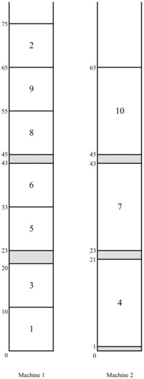
Figure 4.
An optimal C-schedule .
4.3. The Description of the Algorithm and Its Correctness
We give the following Algorithm 1 and prove its correctness:
| Algorithm 1 Blesscmore Algorithm |
| Step 1: Set and . Step 2: If the condition of Lemma 1 holds, then return the schedule and stop. Step 3: Set . Step 4: { iterative stopping rules } If in the schedule : either (i) there exists no regular emerging job and no job from block is stuck, or (ii) there is neither regular nor passive emerging job (there may exist a stuck job in block ), or (iii) there occurs an EIA(a), then return a schedule from the tree T with the minimum makespan and stop; Step 5: { normal extension rule }: if in the schedule , there occurs no EIA(b), then , where l is the regular delaying emerging job else { emergency extension rule } if in the schedule there occurs an EIA(b), then , where l is the latest scheduled passive emerging job, and e is the latest applied stuck job in schedule . Step 6: goto Step 3. |
We give the final illustration of the algorithm for our example. At Step 1, we have (Figure 1). Since the condition at Step 2 is not satisfied, , and the normal extension rule is used to generate the C-schedule in Figure 2. Then, similarly, the normal extension rule is used to generate the C-schedule in Figure 3. Since, in the latter schedule , an EIA(b) with job 4 occurs, this job is revised and an alternative C-schedule after the chain of revisions for the passive emerging job 2 is created. The kernel of this schedule consists of jobs 8, 9, and 10 (as that of schedule ) with and . This is the optimal makespan: There is neither a regular emerging job nor a stuck job in the C-schedule . Hence, the stopping rule (i) applies, and the algorithm stops with an optimal solution.
Now, we prove the following theorem:
Theorem 1.
For some stage h, the C-schedule is an optimal schedule .
Proof.
Suppose that the optimality condition in Lemma 1 is not satisfied for the schedule , and let us consider C-schedule of an iteration . Assume schedule is not optimal, and assume first that there is no stuck job in schedule . Then, in any feasible schedule S with a better makespan, the number of jobs scheduled before the kernel in block must be one less than in the latter schedule as otherwise, due to Property 2 and the fact that there is no stuck job in schedule , a job from the kernel cannot have a smaller full completion time in the schedule than job in the schedule (as the jobs of the kernel are already included in an optimal sequence, see Lemma 1). Thus, some job included before the kernel in the schedule must be scheduled after that kernel in the schedule S. We claim that job l is to be a regular emerging job. Indeed, if it is not, then , or/and . If , then, due to inequality and Proposition 2, . Hence, the makespan of any feasible schedule in which job l is scheduled after the kernel cannot be less than that of schedule . Suppose now . If l is not a passive emerging job, then obviously the above reasoning applies again. Suppose l is a passive emerging job, and suppose first that there is no marched job in the block . Then, since the block starts with the kernel (there exists no regular emerging job schedule ), the full completion time of the overflow job is a lower bound on the optimum schedule makespan (this can be seen similarly to Lemma 1). Obviously, the same reasoning applies in case there are marched jobs in the block , but none of them is stuck in schedule .
The above proves the validity of the stopping rule (i) from Algorithm 1. Suppose now that there is neither a regular nor passive emerging job, and there is a stuck job in schedule . Clearly, the full completion time of the overflow job cannot be decreased unless such stuck job is revised. Note that the corresponding C-schedule coincides with an earlier generated C-schedule , for some from the solution tree T. Furthermore, in any feasible schedule having a makespan less than that of the schedule , another job l with is to be applied instead of job e. Moreover, job l should belong to a block, relative to the block , as otherwise the time interval released by the removal of that job from its current execution interval may not yield a right-shift of any job from the block . It follows that job l is a passive emerging job. This proves the stopping rule (ii). The stopping rule (iii) follows from Lemma 2.
It remains to show that the search in the space of the C-schedules is correctly organized. There are two extension rules. The normal extension rule is used at stage h if there exists a regular emerging job in the schedule . In this case, the delaying emerging job l is applied, i.e., . Consider an alternative feasible schedule , where j is another emerging job (above, we have shown that only emerging jobs need to be considered). It is easy to see that the left-shift of the kernel jobs in the schedule cannot be more than that in the schedule , and the forced right-shift for the jobs scheduled after job j in the schedule cannot be less than that of the jobs scheduled after job l in the schedule (recall that ). Hence, the schedule is dominated by the schedule unless job l gets stuck at a later stage . In the latter case, the emergency extension rule revises first job l. In the resultant C-schedule, the passive delaying job converts into a regular delaying emerging job. Then, the emergency extension rule applies this (converted) regular regular delaying emerging job. We complete the proof by repeatedly applying the above reasoning for the normal extension rule. □
5. Performance Analysis
It is not difficult to see that the direct application of Algorithm 1 of the previous section may yield the generation of some redundant C-schedules: the jobs from the same kernel K including the overflow job o may be forced to be right-shifted after they are already “arranged” (i.e., the corresponding emerging job(s) are already applied to that kernel) due to the arrangement accomplished for the kernel preceding kernel K. As a result (because of the application of an emerging job for the kernel ), one or more redundant C-schedules in which a job from the kernel K repeatedly becomes an overflow job might be created. Such an unnecessary rearrangement of the portion of a C-schedule between the kernels and K is avoided by restricting the number of jobs that are allowed to be scheduled in that portion. This number becomes well-defined after the first disturbance of this portion caused by the application of an emerging job for the kernel . This issue was studied in detail for the case of identical machines in [2] (see Section 4.1). It can be readily verified that the basic estimations for the case of identical machines similarly hold for uniform machines. In particular, the number of the enumerated C-schedules remains the same for uniform machines. A complete time complexity analysis requires a number of additional concepts and definitions from [2] and would basically repeat the arguments for identical machines.
Recall that we use a different schedule generation mechanism for identical and uniform machines: the LDT-heuristic applied for the schedule generation in the identical machine environment is replaced by the LDTC-heuristic for the uniform machine environment. LDT-schedules possess a number of nice properties used in the algorithm from [2]. LDTC-schedules also possess such necessary useful properties (Properties 1 and 2) that allowed us to use the basic framework from [2]. While generating an LDT-schedule for identical machines, every next job is scheduled on the next available machine (the next to the last machine m being machine 1) and the starting and completion time of each next scheduled job is not smaller than that of all previously scheduled ones. In some sense, the generalization of these properties are Properties 1 and 2, which still assure that the structural pattern of the generated schedules is kept, and it does not depend on which particular jobs are being scheduled in a particular time interval (note that this would not be the case for an unrelated machine environment). This allowed us to adopt the blesscmore framework from [2] for the uniform machine environment (for instance, intuitively, while restricting the number of the scheduled jobs between two successive kernels, no matter which particular jobs are being scheduled between these kernels).
Another “redundancy issue” occurs when a series of emerging jobs are successively applied to the same kernel K without reaching the desired result, i.e., the applied emerging jobs become new overflow jobs in the corresponding C-schedules (see Section 4.2 in [2]). In Lemma 7 from the latter reference, it is shown that this yields an additional factor of p in the running time of the algorithm. This result also holds for the uniform machine environment. The magnitude p remains valid for the uniform machine environment as the difference between the completion times of two successively scheduled jobs on the same machine cannot be more than p (recall that p is the processing time of any job on the slowest machine m). The desired result follows since the delivery time of each emerging job next applied to kernel K is strictly less than that of the previously applied one (see the proof of Lemma 7 in [2]).
The above results yield the same bound on the number of the enumerated C-schedules as in [2]), where can be either n or (see Lemma 8 from Section 4.3 and Theorem 2 from Section 6.1, in [2]). In fact, is the total number of the applied emerging jobs, a magnitude that can be essentially smaller than n. This yields the overall cost due to the cost of the LDTC-heuristic (instead of for the LDT-heuristic). A further refinement of the overall time complexity accomplished in [2] is not possible for the uniform machine environment. In the algorithm from [2], while generating every next C-schedule, instead of applying the LDT-heuristic to the whole set of jobs, it is only applied to the jobs from a small part of the current C-schedule, the so-called critical segment (a specially determined part of the latter schedule containing its kernel), and the remaining jobs are scheduled in linear time just by right-shifting the jobs following the critical segment by the required amount of time units (conserving their current processing order). This is not possible for uniform machines as such an obtained schedule will not necessarily remain an LDTC-schedule, i.e., a linear time rescheduling will not provide the desired structure.
6. Discussion and Concluding Remarks
We showed that the earlier developed technique for scheduling identical machines can be extended to the uniform machine environment if Condition (1) on the job parameters is satisfied, thus making a step towards the settlement of the complexity status of this long-standing open problem. In particular, the imposed condition reflects potential conflicts that arise in the uniform machine environment but do not arise in the identical machine environment. It is a challenging question whether the removal of Condition (1) results in an NP-hard problem or if it can still be solved in polynomial time, at least, for a fixed number of machines. Although the LDTC-heuristic would not give the desired results if Condition (1) is not satisfied, it might still be possible to develop a more intelligent heuristic that can successfully be combined with the blesscmore framework and the analysis of the behavior alternatives from [2]. This approach may have some limitations though. As we have mentioned earlier, it is unlikely that it can be applied to the unrelated machine environment, mainly because the structural pattern of the generated schedules will depend on, which particular jobs are scheduled in a particular time interval on each machine from a group of unrelated machines, which makes the analysis of the behavior alternatives much more complicated. At the same time, the approach might be extensible to shop scheduling problems. It is a challenging question whether it can be extended to the case where there are two allowable job processing times (this turned out to be possible for the single-machine environment, see the blesscmore algorithm in [24]) and for a much more general setting with mutually divisible job processing times for identical and uniform machine environments (this turned out to be also possible for the single-machine environment—a maximal polynomially solvable special case of (a strongly NP-hard) problem with mutually divisible job processing times was dealt with recently in [25]). Finally, we note that the algorithm presented here can also be used as an approximate one for non-equal job processing times, as it is often the case in practical applications.
Author Contributions
Conceptualization, N.V.; investigation, N.V. and F.W.; writing—original draft preparation, N.V. and F.W. All authors have read and agreed to the published version of the manuscript.
Funding
The first author is grateful for the support of the DAAD grant 57507438 for Research Stays for University Academics and Scientists.
Institutional Review Board Statement
Not applicable.
Informed Consent Statement
Not applicable.
Data Availability Statement
Not applicable.
Acknowledgments
The authors would like to thank the anonymous referees for useful suggestions and express very special thanks to referee 2 whose very careful comments helped greatly to correct the inconsistencies from the original submission.
Conflicts of Interest
The authors declare no conflict of interest.
References
- Bratley, P.; Florian, M.; Robillard, P. On sequencing with earliest start times and due-dates with application to computing bounds for (n/m/G/Fmax) problem. Nav. Res. Logist. Quart. 1973, 20, 57–67. [Google Scholar] [CrossRef]
- Vakhania, N. A better algorithm for sequencing with release and delivery times on identical processors. J. Algorithms 2003, 48, 273–293. [Google Scholar] [CrossRef]
- Vakhania, N. Branch less, cut more and minimize the number of late equal-length jobs on identical machines. Theor. Comput. Sci. 2012, 465, 49–60. [Google Scholar] [CrossRef]
- Garey, M.R.; Johnson, D.S. Computers and Intractability: A Guide to the Theory of NP-Completeness; Freeman: San Francisco, CA, USA, 1979. [Google Scholar]
- McMahon, G.; Florian, M. On scheduling with ready times and due dates to minimize maximum lateness. Operations 1975, 23, 475–482. [Google Scholar] [CrossRef]
- Carlier, J. The one-machine sequencing problem. Eur. J. Oper. Res. 1982, 11, 42–47. [Google Scholar] [CrossRef]
- Baptiste, P. Scheduling equal-length jobs on identical parallel machines. Discret. Appl. Math. 2000, 103, 21–32. [Google Scholar] [CrossRef]
- Baptiste, P. Polynomial time algorithms for minimizing the weighted number of late jobs on a single machine with equal processing times. J. Sched. 1999, 2, 245–252. [Google Scholar] [CrossRef]
- Chrobak, M.; Dürr, C.; Jawor, W.; Kowalik, L.; Kurowski, M. A note on scheduling equal-length jobs to maximize throughput. J. Sched. 2006, 9, 71–73. [Google Scholar] [CrossRef][Green Version]
- Vakhania, N. A study of single-machine scheduling problem to maximize throughput. J. Sched. 2013, 16, 395–403. [Google Scholar] [CrossRef]
- Vakhania, N. Scheduling jobs with release times premptively on a single machine to minimize the number of late jobs. Oper. Res. Lett. 2009, 37, 405–410. [Google Scholar] [CrossRef]
- Garey, M.R.; Johnson, D.S.; Simons, B.B.; Tarjan, R.E. Scheduling unit-time tasks with arbitrary release times and deadlines. SIAM J. Comput. 1981, 10, 256–269. [Google Scholar] [CrossRef]
- Simons, B.; Warmuth, M.A. Fast algorithm for multiprocessor scheduling of unit-length jobs. SIAM J. Comput. 1989, 18, 690–710. [Google Scholar] [CrossRef]
- Dessouky, M.; Lageweg, B.J.; Lenstra, J.K.; van de Velde, S.L. Scheduling identical jobs on uniform parallel machines. Stat. Neerl. 1990, 44, 115–123. [Google Scholar] [CrossRef]
- Labetoulle, J.; Lawler, E.L.; Lenstra, J.K.; Rinnooy Kan, A.H.G. Preemptive Scheduling of Uniform Machines Subject to Release Dates; Pulleyblank, H.R., Ed.; Progress in Combinatorial Optimization; Academic Press: New York, NY, USA, 1984; pp. 245–261. [Google Scholar]
- Kravchenko, S.; Werner, F. Preemptive scheduling on uniform machines to minimize mean flow time. Comput. Oper. Res. 2009, 36, 2816–2821. [Google Scholar] [CrossRef]
- Lawler, E.L.; Labetoulle, J. On preemptive scheduling of unrelated parallel processors by linear programming. J. Assoc. Comput. Mach. 1978, 25, 612–619. [Google Scholar] [CrossRef]
- Vakhania, N.; Hernandez, J.; Werner, F. Scheduling unrelated machines with two types of jobs. Int. J. Prod. Res. 2014, 52, 3793–3801. [Google Scholar] [CrossRef]
- Lenstra, J.K.; Shmoys, D.B.; Tardos, E. Approximation algorithms for scheduling unrelated machines. Math. Program. 1990, 46, 259–271. [Google Scholar] [CrossRef]
- Brucker, P.; Kravchenko, S. Scheduling Jobs with Release Times on Parallel Machines to Minimize Total Tardiness; OSM Reihe P; Heft 257; Universität Osnabrück: Osnabrück, Germany, 2005. [Google Scholar]
- Brucker, P.; Kravchenko, S. Scheduling jobs with equal processing times and time windows on identical parallel machines. J. Sched. 2008, 11, 229–237. [Google Scholar] [CrossRef]
- Kravchenko, S.; Werner, F. On a parallel machine scheduling problem with equal processing times. Discret. Appl. Math. 2009, 157, 848–852. [Google Scholar] [CrossRef][Green Version]
- Kravchenko, S.; Werner, F. Parallel machine problems with equal processing times: A survey. J. Sched. 2011, 14, 435–444. [Google Scholar] [CrossRef]
- Vakhania, N. Single-Machine Scheduling with Release Times and Tails. Ann. Oper. Res. 2004, 129, 253–271. [Google Scholar] [CrossRef]
- Vakhania, N. Dynamic Restructuring Framework for Scheduling with Release Times and Due-Dates. Mathematics 2019, 7, 1104. [Google Scholar] [CrossRef]


Publisher’s Note: MDPI stays neutral with regard to jurisdictional claims in published maps and institutional affiliations. |
© 2021 by the authors. Licensee MDPI, Basel, Switzerland. This article is an open access article distributed under the terms and conditions of the Creative Commons Attribution (CC BY) license (http://creativecommons.org/licenses/by/4.0/).