Modeling and Semi-Analytic Stability Analysis for Dynamics of AC Machines

Abstract

In this article, a semi-analytical technique is proposed to predict stable sustained periodic responses of AC electrical machines. Based on such desired outputs, the proper selections of machine variables are captured, such as the perturbation parameter arisen from the relative movement between the stationary and rotating parts. Compared to the experimental results, the derived analytical results are relatively well-fitted with the studied practical cases.

1. Introduction

In electrical engineering, the development of electrical systems, such as AC electrical machines, some reliable mathematical models are needed that take into account their theory. Such a model should cover the different views on an interested system as well as the different degrees of detailing that leads from a hierarchy of model to a hierarchy of design system parameters. The specific views of such a system represent the relevant effects of specific interests, such as dynamics, stability, and control, which are used as interfaces for the design engineers during their works. Thus, a validation of the mathematical model is needed, then, a solution response with the experimental system results over the entire range of system interests or for the considered range of switching system parameters have to be compared, cf. [1,2,3].

The solving process for validation can be managed mathematically by various analytical or numerical approaches. In fact, numerical simulations are often necessary in order to understand the attitude response and control characteristics of complex systems; however, the typical problems in numerical simulations are the short time visualization and error analysis, since it may be prohibitively expensive and time consuming, especially when large numbers of parameters are involved. In contrast, analytical descriptions can be of great help in obtaining a qualitative understanding of the complex dynamical behavior, even simple heuristic analytical results may provide a fast and relatively accurate form for maneuver analysis, cf. [4,5,6,7]. For instance, in most engineering control applications, it appears that the trend for autonomous engineering control schemes dictate the use of compact, simple, and analytical expression responses for evolutionary systems, cf. [8,9,10].

Typically, semi-analytical approaches and perturbation methods are used to solve such kinds of models. Recently, some new and emerging approaches were proposed to handle both nonlinear and linear systems with varying coefficients or to consider large parameters and domains of definition as well. Among these approaches that are employed for solving complex systems are the perturbation-iteration method (PIM), variational iteration method (VIM), homotopy analysis method (HAM), and the homotopy perturbation method (HPM), cf. [11,12,13,14,15]. Moreover, there are some improved homotopic approaches, such as the optimal homotopy perturbation method (OHPM) and the optimal homotopy asymptotic method (OHAM); it is worth mentioning the modified differential transform method (MDTM), which is particularly settled in solving boundary values problems, cf. [16,17,18,19]. Most of such approaches have been successfully applied in solving numerous linear and nonlinear problems in science and engineering.

In industrial electrical induction/synchronous machines, mathematical formulations have been carried out in the simulation field, including some internal generated effects such as the rotor temperature, the relative movement or the magnetic saturation with a view to obtaining highly accurate results of output or control, cf. [20,21,22,23]. As often as to simplify the electrical construction of these machines, electrical circuits are rigorous simple models used to exhibit the behavior of their outputs. Indeed, it can be considered as very efficient alternative tools to express massive laboratory experiments for their practical purposes, cf. [24,25,26,27,28].

In this work, the simplification of electrical construction of induction/synchronous machines taking into account the relative movement between the stationary and rotating parts using an RLC circuit modeling is considered. In this case, the electrical circuit system has allowed us simply to derive the governing equation containing the effect of relative movement by using varying inductance expression. At that time, using the ease of handling by circuit modeling, semi-analytical expression for the machine response and the configuration stability are captured.

The use of analytical expression via one of the mentioned approaches is limited to isolate some cases in which the natural response of the governing equation can be expressed explicitly in terms of functions in time, or, at least, it can be reduced to cases of quadratures. The variational iteration technique was found a very efficient tool to form the governing equation to its quadrature form, and the solution might be expressed by terms of iterated integrations, cf. [29,30,31]. The obtained solution by this method captures all values of circuit parameters with large domains of definitions. As far as in specific domains of definitions for some circuit parameters, some special approximate expressions of the solution in terms of time can be initiated by using special methods such as Frobenius method and Poincare–Linstedt approach, which are constructed on specific domains of some parameters, cf. [32,33,34,35].

The benefit of the isolated possible cases, obtained from (semi)analytical solutions shared the property of having them as meromorphic functions of time, might be a very efficient indicator for the stability of the modeled machines. Hence, it turned out that necessary conditions for the sustained periodic motions of the electrical machines ought to be explicitly recognized.

In the present paper, we report on the analytical investigation of the AC machine response using a prototype modeling via modified variational iteration methods (VIM) in terms of iterated meromorphic functions of time. Our contribution is concentrated on the mathematical aspects of that method to obtain the stability domains as well as the transition curves of the governing equation for a wide range of values for the related system parameters. More concretely, our attention is focused on the existence of sustained periodic oscillations represented by the boundary curves to describe stable periodic natural responses using the energy-rate function.

The paper is divided into three sections. In Section 2, the governing system is obtained using the circuital RLC series modeling. In Section 3, the construction of semi-analytical solutions are given via the variational iteration method. In Section 4, stability charts using the concluded resulted from the previous sections are drawn via energy-rate approach. In the last section, the conclusion is given.

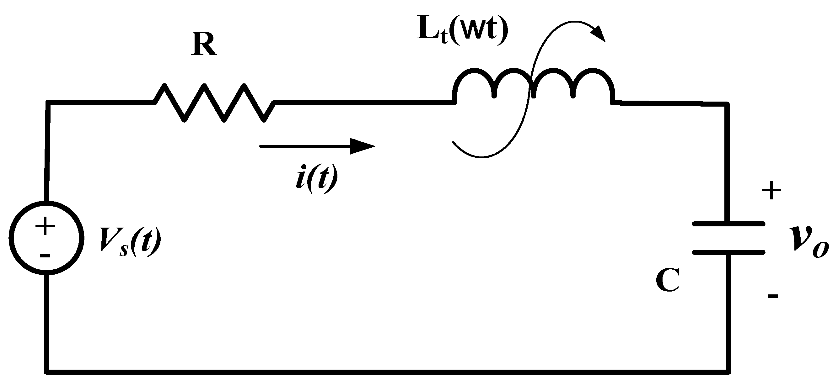
2. The Governing Dynamic Model

Typically, the basic operation of many types of electrical induction/synchronous machines relies on periodic variation of inductance in time. Self-excitation of induction generators can be achieved when connecting machine terminals to sufficient amount of capacitance that depends on the driving rotor speed and load conditions, cf. [36]. The three-phase machines have been successfully analyzed using well-known approaches that depend on d-q transformation, cf. [37]. However, single-phase operation is difficult to analyze using conventional methods. A single-phase parametric generator is modeled as an RLC circuit with periodically time varying inductance, cf. [38]. This type of generator is expected to be suitable for energy harvesting applications, e.g., electrical generation from wave energy. Practically, the inductance variation can be attained through variation of magnetic coupling between two series-connected coils; one is fixed while the other is rotating as shown in Figure 1.

From the basic laws of electrical circuits and Figure 2, the voltage equation of the RLC-series circuit is given by the following equation,

$${\displaystyle \frac{d}{dt}}(L_{t}i(t))+R_{t}i(t)+{\displaystyle \frac{1}{C_t}}{\int }_0^{t}i(t)dt=V_s(t),$$

(1)

where t, $i(t)$, $V_s(t)$ are the time, the electric current, and the supply, respectively. The coefficients $L_t(i,t)$, $R_t(i,t)$ and $C_t(i,t)$ are the inductance, the resistance and capacitance functions in time, and the electric current.

By considering that the resistance and the capacitance are constant and the inductance varies periodically with time due to the existence of relative movement between the stator and the rotor of such AC machine, some loop inductances of AC machines depend upon the rotor position. Hence, the governing equation takes the following form

$${\displaystyle \frac{d}{dt}}(L_t(t)i(t))+Ri(t)+{\displaystyle \frac{1}{C}}{\int }_0^{t}i(t)dt=V_s(t),$$

(2)

regardless of the power measurement and control accessories.

For simplicity, let us define the following new variables in terms of the angle $x=\omega t$ in the natural response of the system,

$$i(x)=\frac{1}{\omega }\frac{dq}{dx},q(x)=\frac{1}{\omega }\frac{dy}{dx},i(x)=\frac{1}{{\omega }^2}\frac{d^{2}y}{d{x}^2}.$$

(3)

where q and $\omega$ are the charge and the angular frequency respectively. Let us introduce the time varying inductance as,

$$L_t(x)=L_{0}F(x),$$

(4)

where $L_0$ is the reference value of the inductance and $F(x)$ is considered as predictable function for the studied AC machine.

Including the new variables in the homogeneous part, we obtain

$${\displaystyle \frac{d}{dx}}(L_t{y}^{″})+\frac{R}{\omega }{y}^{″}+{\displaystyle \frac{1}{{\omega }^{2}C}}{y}^{\prime }=0.$$

(5)

Integrating both sides once, taking into the account the natural response only, hence we get

$$L_t{y}^{″}+\frac{R}{\omega }{y}^{\prime }+{\displaystyle \frac{1}{{\omega }^{2}C}}y=0.$$

(6)

Hence, dividing both sides by $L_0$, it yields

$$F(x)y^{″}+{\displaystyle \frac{R}{\omega L_0}}{y}^{\prime }+\frac{1}{L_0{\omega }^{2}C}y=0.$$

(7)

By considering that

$$\begin{array}{c}\hfill {\omega }_0={\displaystyle \frac{1}{\sqrt{L_{0}C}}}>0,\alpha ={\displaystyle \frac{\omega }{{\omega }_0}}>0,Q={\displaystyle \frac{R}{{\omega }_0{L}_0}}\ge 0,\end{array}$$

then, we obtain

$$F(x)y^{″}+{\displaystyle \frac{Q}{\alpha }}{y}^{\prime }+{\displaystyle \frac{1}{{\alpha }^2}}y=0.$$

(8)

If the predictable function of inductance is considered periodically time dependent as follows

$$F(x)=1+hcos2x,$$

(9)

where h is the perturbation parameter arisen from the dynamic perturbation on the inductance due the relative movement between stator and rotor of the machine.

Now, the governing equation of the modeling circuit described by a linear model as follows

$$(1+hcos2x)y^{″}+{\displaystyle \frac{Q}{\alpha }}{y}^{\prime }+{\displaystyle \frac{1}{{\alpha }^2}}y=0.$$

(10)

Hence, the governing equation of the natural response reads

$$(1+hcos2x)y^{″}+{\displaystyle \frac{Q}{\alpha }}{y}^{\prime }+{\displaystyle \frac{1}{{\alpha }^2}}y=0,y(0)=c_1,y^{\prime }(0)=c_2,$$

(11)

where $c_1$ and $c_2$ are real constants representing the values of variants y and its derivative at the initial angular position of the rotor oscillatory movement. Indeed, the solution ($y(x)$) of Equation (11) represents the net positive charge that moved past an instantaneous point in a specified direction in the shown circuit under the specified initial conditions and the absence of the voltage supply ($V_s$), cf. [5].

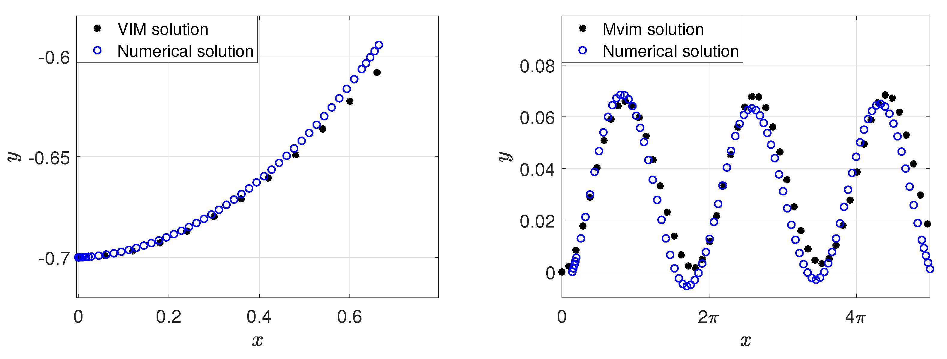
3. Construction of Semi-Analytical Solutions via VIM

In this section, the explicit algebraic solutions as meromorphic functions of time and the rough analytical analysis of stability are given. Particularly, in accordance with the existence of large domains of perturbation parameter (h), approximate forms of the solution are needed to construct. Consequently, the curves containing a stable periodic characterization might be drawn.

Variational iteration method is needed as a general method to capture the behavior of solutions for a large scale of h. This method is an efficient technique to construct general solutions and not influenced by inherent variation of problem parameters, cf. [39]. Consequently, the yielded solutions describe the behavior of the governing equation in neighborhoods of boundary curves and upon them.

Consider the following differential equation (DE)

$$Ly(x)+Ny(x)=f(x),$$

(12)

where L and N are linear and nonlinear operators, respectively, and $f(x)$ is the source of inhomogeneous term. The method admits the use of a correction functional for Equation (12) in the form

$$y_{n+1}(x)=y_n(x)+{\int }_0^x\lambda (t)(L{y}_n(t)+N\tilde{y}(t)-f(t))dt,$$

(13)

where $\lambda$ is a general Lagrange’s multiplier, which can be identified optimally via variational theory, $\tilde{y}(t)$ is a restricted variational such that $\delta \tilde{y}(t)=0$. Lagrange’s multiplier is very critical in this method and it can be constant or function according to equation and conditions of it, the zeroth approximation $y_0$ can be any function, using the initial values $y(0),y^{\prime }(0)$ and $y^{″}(0)$ are preferable used for the selective zeroth approximation $y(0)$.

The final solution is given by

$$y(x)=\underset{n\to \infty }{lim}{y}_n(x).$$

(14)

Now the general second order differential equation can be written as

$$y^{″}(x)+a(x)y^{\prime }(x)+b(x)y(x)=0.$$

(15)

Following [14,15,31,40,41], then VIM admits the use of the correction functional for this equation by

$$y_{n+1}(x)=y_n(x)+{\int }_0^x\lambda (t)(y_n^{″}(t)+a(t){\tilde{y}}_n^{\prime }(t),+b(t){\tilde{y}}_n(t))dt,$$

(16)

where

$$\begin{array}{c}\hfill y(0)=c_1,y^{\prime }(0)=c_2.\end{array}$$

Taking the variation of both sides of Equation (16) with respect to independent variable $y_n(x)$, we find

$${\displaystyle \frac{\delta y_{n+1}}{\delta y_n}}=1+{\displaystyle \frac{\delta }{\delta y_n}}{\int }_0^x\lambda (t)(y_n^{″}(t)+a(t){\tilde{y}}_n^{\prime }(t)+b(t){\tilde{y}}_n(t))dt,$$

(17)

or equivalently

$$\delta y_{n+1}(x)=\delta y_n(x)+\delta {\int }_0^x\lambda (t)(y_n^{″}(t)+a(t){\tilde{y}}_n^{\prime }(t)+b(t){\tilde{y}}_n(t))dt.$$

(18)

Using $\delta {\tilde{y}}_n^{\prime }(t)=0$, $\delta {\tilde{y}}_n(t)=0$ that gives

$$\delta y_{n+1}(x)=\delta y_n(x)+\delta ({\int }_0^x\lambda (t)y_n^{″}(t)dt).$$

(19)

Integrating Equation (19) by parts twice gives

$$\begin{array}{cc}\hfill \delta y_{n+1}(x)=& \delta y_n(x)+(\delta \lambda (t)y_n^{\prime }(t)-\delta \lambda {(t)}^{\prime }{y}_n(t)){|}_0^x\hfill \\ & +\delta {\int }_0^x{\lambda }^{″}(t)y_n(t)dt.\hfill \end{array}$$

(20)

This is equivalent to

$$\delta y_{n+1}(x)=\delta (1-{\lambda }^{\prime }{|}_{t=x})y_n(x)+\delta \lambda {|}_{t=x}{y}_n^{\prime }(x)+\delta {\int }_0^x{\lambda }^{″}(t)y_n(t)dt,$$

(21)

$\delta y_{n+1}(x)=0$. This means that the left side of Equation (21) is 0, and the right side of Equation (21) should be 0 as well.

Thus, this yields the following stationary conditions

$$\begin{array}{cc}\hfill & 1-{\lambda }^{\prime }{|}_{t=x}=0,\hfill \end{array}$$

(22)

$$\begin{array}{cc}\hfill & \lambda {|}_{t=x}=0,\hfill \end{array}$$

(23)

$$\begin{array}{cc}\hfill & {\lambda }^{″}{|}_{t=x}=0.\hfill \end{array}$$

(24)

This in turn gives

$$\lambda =t-x.$$

(25)

Substituting this values of $\lambda$ into Equation (16) gives the iteration formula

$$\begin{array}{cc}\hfill y_{n+1}(x)=y_n(x)+{\int }_0^x& (t-x)(y_n^{″}(t)+a(t)y_n^{\prime }(t)\hfill \\ & +b(t)y_n(t))dt,\hfill \end{array}$$

(26)

such that $y(0)=c_1,y^{\prime }(0)=c_2$ and

$$y_0(x)=c_1+c_{2}x.$$

(27)

We find the solution of the system Equation (15) by using the iteration formula Equation (26)

$$\begin{array}{cc}\hfill y_{n+1}(x)=y_n(x)+{\int }_0^x& (t-x)(y_n^{″}(t)+{\displaystyle \frac{Q}{\alpha (1+hcos2t)}}{y}_n^{\prime }(t)\hfill \\ & +{\displaystyle \frac{1}{{\alpha }^2(1+hcos2t)}}{y}_n(t))dt,\hfill \end{array}$$

(28)

where $y_0(x)=y_0$

$$y_1(x)=y_0+{\displaystyle \frac{y_0}{{\alpha }^2}}{\int }_0^x{\displaystyle \frac{(t-x)}{1+hcos2t}}dt,$$

(29)

$$\begin{array}{cc}\hfill {\int }_0^x{\displaystyle \frac{(t-x)}{1+hcos2t}}dt=& [-(h^2-1)L{i}_2{\displaystyle \frac{hcos2x+isin2x}{\sqrt{1-h^2}-1}}\hfill \\ & +(h^2-1)L{i}_2{\displaystyle \frac{-(hcos2x+isin2x)}{\sqrt{1-h^2}+1}}\hfill \\ & +4i\sqrt{-{(h^2-1)}^2}x{tan}^{-1}{\displaystyle \frac{ihsin(2x)+hcos(2x)+1}{\sqrt{h^2-1}}}\hfill \\ & -2i(h^2-1)xlog(1-{\displaystyle \frac{hcos2x+isin2x}{\sqrt{1-h^2}-1}})\hfill \\ & -log(1+{\displaystyle \frac{hcos2x+isin2x}{\sqrt{1-h^2}-1}})]/(4\sqrt{h^2+1}\sqrt{-{(h^2-1)}^2}.\hfill \end{array}$$

(30)

where $L{i}_s$ is the polylogarithm function and is defined by a power series in z, which is also a Dirichlet series in s:

$$L{i}_s(z)=\sum _{k=1}^{\infty }{\displaystyle \frac{z^k}{k^s}}.$$

(31)

Thus, to overcome the difficulty of integration term, we can use the transformation

$${\int }_0^x{\displaystyle \frac{(t-x)}{1+hcos2t}}dt={\int }_0^x{\displaystyle \frac{(t-x)}{1+h(1-2t^2+\frac{2}{3}{t}^4+...)}}dt,$$

(32)

then

$$\begin{array}{cc}\hfill y_1(x)=& y_0+{\displaystyle \frac{y_0}{{\alpha }^2}}{\displaystyle \frac{\sqrt{3}}{4\sqrt{h-2}}}[{\displaystyle \frac{2\sqrt{2}x}{\sqrt{-3h-\sqrt{3h(h-2)}}}}\hfill \\ & {tan}^{-1}({\displaystyle \frac{\sqrt{2h}x}{\sqrt{-3h-\sqrt{3h(h-2)}}}})+{\displaystyle \frac{2\sqrt{2}x}{\sqrt{-3h+\sqrt{3h(h-2)}}}}\hfill \\ & {tan}^{-1}({\displaystyle \frac{\sqrt{2h}x}{\sqrt{-3h+\sqrt{3h(h-2)}}}})\hfill \\ & +log{\displaystyle \frac{-2\sqrt{h}{x}^2+\sqrt{3(h-2)}+3\sqrt{h}}{\sqrt{h}}}\hfill \\ & -log{\displaystyle \frac{2\sqrt{h}{x}^2+\sqrt{3(h-2)}-3\sqrt{h}}{\sqrt{h}}}\hfill \\ & -log{\displaystyle \frac{\sqrt{3(h-2)}+3\sqrt{h}}{\sqrt{h}}}+log{\displaystyle \frac{\sqrt{3(h-2)}-3\sqrt{h}}{\sqrt{h}}}...]\hfill \end{array}$$

(33)

From the first approximation (Equation (33)), it seems very predictable for the aperiodic solutions, but for the periodic ones, the treatment should involve them.

In the case of $\left|h\right|<1$, we can use the transformation

$${\int }_0^x{\displaystyle \frac{(t-x)}{1+hcos2t}}dt={\int }_0^x(t-x)(1-hcos2t+h^2{cos}^2(2t)-h^3{cos}^3(2t)...)dt,$$

(34)

then

$$\begin{array}{cc}\hfill y_1(x)=& y_0-{\displaystyle \frac{y_0}{36{\alpha }^2}}(9(h^2+2)x^2+9h(2h^2-h+2){sin}^2(x)\hfill \\ & -3h^2(-4h+3){sin}^4(x)-8h^3{sin}^6(x)).\hfill \end{array}$$

(35)

For further simplification, it reads

$$\begin{array}{cc}\hfill y_1(x)=& y_0+{\displaystyle \frac{y_0}{288{\alpha }^2}}(h^2(56h+9)+72h-72(h^2+2)x^2\hfill \\ & -18h(3h^2+4)cos2x+9h^{2}cos4x-2h^{3}cos6x)+....\hfill \end{array}$$

(36)

The second approximation ($n=1$) can be obtained as

$$\begin{array}{c}\hfill y_2(x)=y_0+{\displaystyle \frac{1}{1382400{\alpha }^3}}(Q{A}_1+{\displaystyle \frac{12}{\alpha }}{A}_2)+....\end{array}$$

(37)

where

$$\begin{array}{cc}\hfill A_1=& -120h^2(-832h^3+675h^2+2240h+720)x-57600{(h^2+2)}^2{x}^3\hfill \\ & -172800h(h^2+2)xcos2x-7200h(5h^4+3h^2-24)sin2x\hfill \\ & +21600h^2(h^2+2)xcos4x+1800h^2(7h^2+6)sin4x\hfill \\ & -4400h^3(h^2+2)sin6x+1125h^{4}sin8x-144h^{5}sin10x,\hfill \end{array}$$

(38)

$$\begin{array}{cc}\hfill A_2=& 513088h^5+654075h^4+2955200h^3-259200(2{\alpha }^2-3)h^2\hfill \\ & +4147200({\alpha }^2+1)h-7200x^2(h(h(112h^3+99h^2+368h\hfill \\ & +576{\alpha }^2+108)-288)+1152{\alpha }^2)+172800{(h^2+2)}^2{x}^4\hfill \\ & +7200h(144(h^2+2)x^2-(82h^4+112h^3+423h^2\hfill \\ & +144h+576{\alpha }^2+576))cos2x-2073600h(h^2+2)xsin2x\hfill \\ & +1800h^2(-72(h^2+2)x^2+56h^3+83h^2+72h+288{\alpha }^2+144)\hfill \\ & cos4x+129600h^2(h^2+2)xsin4x-800h^3(29h^2+49)cos6x\hfill \\ & +2925h^{4}cos8x-288h^{5}cos10x.\hfill \end{array}$$

(39)

Regarding the case of $\left|h\right|<1$, the modified VIM method (MVIM) using the linear function of Lagrange multiplier can be modified to obtain a general periodic characterization. We should search for Lagrange’ multiplier to maintain this property. To overcome this difficulty, we can use the following transformation represented by

$${\displaystyle \frac{1}{{\alpha }^2(1+hcos2x)}}={\displaystyle \frac{1}{{\alpha }^2}}+{\displaystyle \frac{1}{{\alpha }^2}}[-hcos2x+h^2{cos}^{2}2x-...].$$

(40)

Then, the governing equation is converted to the following

$$y^{″}+{\displaystyle \frac{1}{{\alpha }^2}}y+{\displaystyle \frac{Q}{\alpha (1+hcos2x)}}{y}^{\prime }+{\displaystyle \frac{1}{{\alpha }^2}}[-hcos2x+h^2{cos}^{2}2x-...]y=0.$$

(41)

Following [29,40,41], the modified VIM admits the use of the correction functional by

$$\begin{array}{cc}\hfill y_{n+1}(x)=y_n(x)+({\int }_0^x& \lambda (t)(y_n^{″}(t)+{\displaystyle \frac{1}{{\alpha }^2}}{y}_n(x)+a(t){\tilde{y}}_n^{\prime }(t)\hfill \\ & +b(t){\tilde{y}}_n(t)dt),\hfill \end{array}$$

(42)

where

$$\begin{array}{c}\hfill y(0)=c_1,y^{\prime }(0)=c_2\end{array}$$

Taking the variation of both sides of Equation (42) with respect to independent variable $y_n(x)$, we find

$$\begin{array}{cc}\hfill {\displaystyle \frac{\delta y_{n+1}}{\delta y_n}}=1+{\displaystyle \frac{\delta }{\delta y_n}}({\int }_0^x& \lambda (t)(y_n^{″}(t)+{\displaystyle \frac{1}{{\alpha }^2}}{y}_n(t)+a(t){\tilde{y}}_n^{\prime }(t)\hfill \\ & +b(t){\tilde{y}}_n(t)dt),\hfill \end{array}$$

(43)

or equivalently

$$\begin{array}{cc}\hfill \delta y_{n+1}(x)=\delta y_n(x)+\delta ({\int }_0^x& \lambda (t)(y_n^{″}(t)+{\displaystyle \frac{1}{{\alpha }^2}}{y}_n(t)+a(t){\tilde{y}}_n^{\prime }(t)\hfill \\ & +b(t){\tilde{y}}_n(t)dt).\hfill \end{array}$$

(44)

Using $\delta {\tilde{y}}_n^{\prime }(t)=0$, $\delta {\tilde{y}}_n(t)=0$ gives

$$\delta y_{n+1}(x)=\delta y_n(x)+\delta ({\int }_0^x(\lambda (t)y_n^{″}(t)+{\displaystyle \frac{1}{{\alpha }^2}}{y}_n(t)dt).$$

(45)

Integrating Equation (45) by parts twice to give

$$\begin{array}{cc}\hfill \delta y_{n+1}(x)=& \delta y_n(x)+(\delta \lambda (t)y_n^{\prime }(t)-\delta \lambda {(t)}^{\prime }{y}_n(t)){|}_0^x\hfill \\ & +\delta {\int }_0^x({\lambda }^{″}(t)+{\displaystyle \frac{1}{{\alpha }^2}})y_n(t)dt.\hfill \end{array}$$

(46)

This is equivalent to

$$\begin{array}{cc}\hfill \delta y_{n+1}(x)=& \delta (1-{\lambda }^{\prime }{|}_{t=x})y_n(x)+\delta \lambda {|}_{t=x}{y}_n^{\prime }(x)\hfill \\ & +\delta {\int }_0^x({\lambda }^{″}(t)+{\displaystyle \frac{1}{{\alpha }^2}})y_n(t)dt,\hfill \end{array}$$

(47)

$\delta y_{n+1}(x)=0$, this mean that the left side of Equation (47) is 0 and so the right side of the equation should be 0 as well. This yields the following stationary conditions

$$\begin{array}{cc}\hfill & 1-{\lambda }^{\prime }{|}_{t=x}=0,\hfill \end{array}$$

(48)

$$\begin{array}{cc}\hfill & \lambda {|}_{t=x}=0.\hfill \end{array}$$

(49)

$$\begin{array}{cc}\hfill & {\lambda }^{″}+{\displaystyle \frac{1}{{\alpha }^2}}{|}_{t=x}=0.\hfill \end{array}$$

(50)

This in turn gives

$$\lambda =\alpha sin({\displaystyle \frac{1}{\alpha }}(t-x)).$$

(51)

Substituting this value of $\lambda$ into Equation (42) to give the iteration formula.

$$\begin{array}{cc}\hfill y_{n+1}(x)=y_n(x)+\alpha {\int }_0^x& sin({\displaystyle \frac{1}{\alpha }}(t-x))(y_n^{″}(t)+{\displaystyle \frac{1}{{\alpha }^2}}{y}_n(x)\hfill \\ & +a(t)y_n^{\prime }(t)+b(t)y_n(t))dt,\hfill \end{array}$$

(52)

such that $y(0)=c_1,y^{\prime }(0)=c_2$ and $y_0(x)=c_1+c_{2}x$

$$\begin{array}{cc}\hfill y_{n+1}(x)=y_n(x)+\alpha {\int }_0^x& sin({\displaystyle \frac{1}{\alpha }}(t-x))[y_n^{″}(t)\hfill \\ & +{\displaystyle \frac{Q}{\alpha (1+hcos2t)}}{y}_n^{\prime }(t)\hfill \\ & +{\displaystyle \frac{1}{{\alpha }^2(1+hcos2t)}}{y}_n(t)]dt,\hfill \end{array}$$

(53)

where $y_0(x)=y_0$. Hence,

$$\begin{array}{cc}\hfill y_1(x)=& y_0+{\displaystyle \frac{y_0}{2(4{\alpha }^2-1)(16{\alpha }^2-1)}}[h^2(-64{\alpha }^4+20{\alpha }^2-1)\hfill \\ & -128{\alpha }^4+40{\alpha }^2-2+(4{\alpha }^2-1)h^{2}cos(4x)\hfill \\ & -(32{\alpha }^2-2)hcos(2x)+[h^2(64{\alpha }^4-24{\alpha }^2+2)\hfill \\ & -h(2-32{\alpha }^2)+128{\alpha }^4-40{\alpha }^2+2]cos(\frac{x}{\alpha })].\hfill \end{array}$$

(54)

The verification of the obtained semi-analytical solutions with the corresponding numerical solutions are vividly shown in Figure 3. The asymptotic characterization of the response of Equation (11) is strongly verified numerically using the 4th order Rung–Kutta algorithm with the shown initial values. As it is clearly shown in the comparison, the semi-analytical solution is comparable with the numerical one at different values of the perturbation parameter. All results exhibit mostly that the stability characterization achieved merely in the domain of definition: $\left|h\right|<1$, which is coinciding with the results in [5,38].

4. Construction of Stability Domains

Several techniques are used to predict the stability of systems, cf. [42,43,44,45,46,47]. Based on the constructed semi-analytical solutions, it is readily to apply the energy-rate method to obtain three dimensional illustration of stability surface showing a sense of relative stability of parameter plane, cf. [48,49,50]. Based on the shown figure, Figure 3, the stability regions lie on the domain $\left|h\right|<1$. So that the intersection of a zero plane with stability surface coming from the solution in $\left|h\right|<1$ determines the boundary curves of the system. The energy-rate function for our system reads

$$\Gamma (h,Q,\alpha )=\frac{1}{T}{\int }_0^T\dot{\mathbb{E}}dx,$$

(55)

where $\mathbb{E}$ is the mechanical energy of the system, and represents the instantaneous rate of generated or absorbed energy by the applied force

$$F=-hcos2x{y}^{″}-\frac{Q}{\alpha }{y}^{\prime }.$$

(56)

Then the energy-rate function can be calculated by

$$\Gamma (h,Q,\alpha )=\frac{1}{T}{\int }_0^T(-hcos2x{y}^{″}-\frac{Q}{\alpha }{y}^{\prime })dy.$$

(57)

The energy-rate function is zero for free vibration of a conservative system, as well as the steady state T-periodic response of the system. Equation (57) includes three parameters, h, Q, and $\alpha$; therefore, the parameter space is two-dimensional if Q is fixed. Determination of the stability domains is carried out by finding the pairs of $(\alpha ,h)$ located on the boundary of stable domains for every fixed value of Q. Plugging the semi-analytical solution represented by Equation (53) and Equation (54) for the case of $\left|h\right|<1$ in Equation (57) and by using the iterative symbolic computations of Maple program, then we get the value of the energy-rate ($\Gamma$) as function of h, $\alpha$ and Q(omitted here for brevity due to its long form).

Analogous to the mechanical system if $\Gamma >0$, then the energy is being inserted to the system and the point $(\alpha ,h)$ belongs to an unstable domain. In contrast, if $\Gamma <0$, then the energy is being extracted from the system and the point $(\alpha ,h)$ belongs to a stable domain. In the case of $\Gamma =0$, common boundaries of these two domains are appeared called transition curves. So that, in the case of zero energy-rate, we look for the transition curves by the relation between $\alpha$ and h at fixed values of Q with the period $T=\pi$ or $T=2\pi$ according to Floquet’s theory, cf. [5]. The resulting figure at $\Gamma$ in the domain $\left|h\right|<1$ is shown in Figure 4 starting with the value of $(0,1)$. These results have relative agreement with the experimental work on AC synchronous machines shown in [26,38,51].

5. Conclusions

In this work, the modeling of AC machines has been dealt with, taking into account the existence of the effect of relative movements between the stators and rotors, such as the RLC electric circuits with periodically time varying inductance. Semi-analytic solutions are obtained for the circuit responses via the modified variational iteration method. In that case of study, the resulting solutions are likely to be valid for large domains of definitions of parameters in the governing system. Within the domain $\left|h\right|<1$, the stability domains are recognized using the zero surface of energy-rate function to represent the transition curves between the stable and unstable regions. This result was shown on a wide variety of practical and experimental literature of the studied problem. Moreover, the relationships among the circuit parameters for stable sustained periodic outputs are configured.

References

1. De Lacalle, L.N.L.; Lamikiz, A.; Sanchez, J.A.; de Bustos, I.F. Simultaneous measurement of forces and machine tool position for diagnostic of machining tests. IEEE Trans. Instrum. Meas. 2005, 54, 2329–2335. [Google Scholar]
2. Hehenberger, P.; Poltschak, F.; Zeman, K.; Amrhein, W. Hierarchical design models in the mechatronic product development process of synchronous machines. Mechatronics 2010, 20, 864–875. [Google Scholar] [CrossRef]
3. Riel, T.; Saathof, R.; Katalenic, A.; Ito, S.; Schitter, G. Noise analysis and efficiency improvement of a pulse-width modulated permanent magnet synchronous motor by dynamic error budgeting. Mechatronics 2018, 50, 225–233. [Google Scholar] [CrossRef]
4. Abdel-Halim, I.A.M.; Ahmar, M.; El-Sherif, M.Z. A novel approach for the analysis of self-excited induction generators. Electr. Mach. Power Syst. 1999, 27, 879–888. [Google Scholar] [CrossRef]
5. El-Borhamy, M.; Rashad, E.M.; Sobhy, I. Floquet analysis of linear dynamic RLC circuits. Open Phys. 2020, 18, 264–277. [Google Scholar] [CrossRef]
6. Herisanu, N.; Marinca, V.; Madescu, G.; Dragan, F. Dynamic response of a permanent magnet synchronous generator to a wind gust. Energies 2019, 12, 915. [Google Scholar] [CrossRef] [Green Version]
7. Matusita, K.; Omatu, S. Use of the homotopy method for excitation control of generators for multimachine power system. Electr. Eng. Jpn. 1996, 117, 96–111. [Google Scholar] [CrossRef]
8. Longuski, J.M.; Tsiotras, P. Analytical solutions for a spinning rigid body subject to time-varying body-fixed torques, part 1: Constant axial torque. J. Appl. Mech. 1993, 60, 970–975. [Google Scholar] [CrossRef]
9. Monje, C.A.; Chen, Y.; Vinagre, B.M.; Xue, D.; Feliu, V. Fractional-Order Systems and Controls: Fundamentals and Applications; Springer Science & Business Media: Berlin/Heidelberg, Germany, 2010. [Google Scholar]
10. Wilkinson, S.A.; Vogt, N.; Golubev, D.S.; Cole, J.H. Approximate solutions to Mathieu’s equation. Physica E 2018, 100, 24–30. [Google Scholar] [CrossRef] [Green Version]
11. Abbasbandy, S.; Jalili, M. Determination of optimal convergence-control parameter value in homotopy analysis method. Numer. Algorithms 2013, 64, 593–605. [Google Scholar] [CrossRef]
12. Aksoy, Y.; Pakdemirli, M.; Abbasbandy, S.; Boyaci, H. New perturbation-iteration solutions for nonlinear heat transfer equations. Int. J. Numer. Methods Heat Fluid Flow 2012, 22, 814–828. [Google Scholar] [CrossRef]
13. Gupta, A.K.; Ray, S.S. Comparison between homotopy perturbation method and optimal homotopy asymptotic method for the soliton solutions of Boussinesq-Burger equations. Comput. Fluids 2014, 103, 34–41. [Google Scholar] [CrossRef]
14. Wazwaz, A.M. The variational iteration method for analytic treatment for linear and nonlinear ODEs. Appl. Math. Comp. 2009, 212, 120–134. [Google Scholar] [CrossRef]
15. Wazwaz, A.M. The variational iteration method for solving linear and nonlinear ODEs and scientific models with variable coefficients. Cent. Europ. J. Eng. 2014, 4, 64–71. [Google Scholar] [CrossRef]
16. Herisanu, N.; Marinca, V. Optimal homotopy perturbation method for a non-conservative dynamical system of a rotating electrical machine. Z. Nat. A 2012, 67, 509–516. [Google Scholar] [CrossRef]
17. Marinca, V.; Herisanu, N. On the flow of a Walters-type B viscoelastic fluid in a vertical channel with porous wall. Int. J. Heat Mass Transf. 2014, 79, 146–165. [Google Scholar] [CrossRef]
18. Marinca, V.; Herisanu, N. The Optimal Homotopy Asymptotic Method; Engineering Applications; Springer: Cham, Switzerland, 2015. [Google Scholar]
19. Rashidi, M.M.; Efrani, E. The modified differential transform method for investigating nano boundary-layers over stretching surfaces. Int. J. Numer. Methods Heat Fluid Flow 2011, 21, 864–883. [Google Scholar] [CrossRef]
20. Ding, H.; Gong, X.; Gong, Y. Estimation of rotor temperature of permanent magnet synchronous motor based on model reference fuzzy adaptive control. Math. Probl. Eng. 2020, 2020, 4183706. [Google Scholar] [CrossRef]
21. Hou, K.; Li, Z.; Chen, L.; Xia, D.; Li, Q.; Xiao, Y. Steady-state stability of sending-end system with mixed synchronous generator and power-electronic-interfaced renewable energy. Math. Probl. Eng. 2020, 2020, 8693245. [Google Scholar] [CrossRef] [Green Version]
22. Jose, J.T.; Chattopadhyay, A.B. Mathematical formulation of feedback linearizing control of doubly fed induction generator including magnetic saturation effects. Math. Probl. Eng. 2020, 2020, 3012406. [Google Scholar] [CrossRef]
23. Zhang, M.; Xiao, F.; Shao, R.; Deng, Z. Robust fault detection for permanent-magnet synchronous motor via adaptive sliding-mode observer. Math. Probl. Eng. 2020, 2020, 9360939. [Google Scholar] [CrossRef]
24. Dehghanzadeh, A.R.; Behjat, V.; Banaei, M.R. Dynamic modeling of wind turbine based axial flux permanent magnetic synchronous generator connected to the grid with switch reduced converter. Ain Shams Eng. J. (ASEJ) 2018, 9, 125–135. [Google Scholar] [CrossRef] [Green Version]
25. Gao, J.; Zhang, L.; Wang, X. AC Machine Systems: Mathematical Model and Parameters, Analysis and System Performance; Springer: Berlin/Heidelberg, Germany, 2009. [Google Scholar]
26. Mostafa, A.S.; Mohamadein, A.L.; Rashad, E.M. Application of Floquet’s theory to the analysis of series-connected wound-rotor self-excited synchronous generator. IEEE Trans. Energy Convers. 1993, 8, 369–376. [Google Scholar] [CrossRef]
27. Nabil, M.; Allam, S.M.; Rashad, E.M. Modeling and design considerations of a photovoltaic energy source feeding a synchronous reluctance motor suitable for pumping systems. Ain Shams Eng. J. (ASEJ) 2012, 3, 375–382. [Google Scholar] [CrossRef] [Green Version]
28. Rashad, E.M. Theory and steady-state analysis of series-connected wound-rotor induction motor in sub-synchronous mode. In Proceedings of the 2016 IEEE International Conference on Power and Energy (PECon), Melaka City, Malaysia, 28–30 November 2016. [Google Scholar]
29. He, J.H. Variational iteration method for autonomous ordinary differential systems. Appl. Math. Comp. 2000, 114, 115–123. [Google Scholar] [CrossRef]
30. He, J.H. Variational iteration method: Some recent results and new interpretations. J. Comp. Appl. Math. 2007, 207, 3–17. [Google Scholar] [CrossRef] [Green Version]
31. He, J.H.; Wu, X.W. Variational iteration method: New development and applications. Comput. Math. Appl. 2007, 54, 881–894. [Google Scholar] [CrossRef] [Green Version]
32. Chicone, C. Ordinary Differential Equations with Applications; Springer Science & Business Media: Berlin/Heidelberg, Germany, 2006. [Google Scholar]
33. Hale, J.K. Ordinary Differential Equations; Dover Publications: Garden City, NY, USA, 2009. [Google Scholar]
34. Nayfeh, A. H Introduction to Perturbation Techniques; John Wiley & Sons: Hoboken, NJ, USA, 2011. [Google Scholar]
35. Shivamoggi, B. Perturbation Methods for Differential Equations; Springer Science & Business Media: Berlin/Heidelberg, Germany, 2012. [Google Scholar]
36. Grantham, C.; Sutanto, D.; Mismail, B. Steady-state and transient analysis of self-excited induction generators. In IEE Proceedings B (Electric Power Applications); IET Digital Library, 1989; Volume 136, pp. 61–68. Available online: https://digital-library.theiet.org/content/journals/10.1049/ip-b.1989.0008 (accessed on 16 March 2021).
37. Krause, P.C.; Wasynczuk, O.; Sudhoff, S.D. Analysis of Electrical Machinery; IEEE Press: New York, NY, USA, 1995. [Google Scholar]
38. Rashad, E.M. Application of Floquet Theory to the Analysis of Parametric Generator. Ph.D. Thesis, Alexandria University, Alexandria, Egypt, 1992. [Google Scholar]
39. He, J.-H. Nonlinear Mathieu equation and its approximation without a small parameter. Engng. Trans. 2002, 50, 43–54. [Google Scholar]
40. Jafari, H.; Alipoor, A. A new method for calculating general Lagrange multiplier in the variational iteration method. Numer. Meth. Partial. Differ. Equ. 2011, 27, 996–1001. [Google Scholar] [CrossRef]
41. Jafari, H.; Saeidy, M.; Baleanu, D. The variational iteration method for solving nth order fuzzy differential equations. Open Phys. 2012, 10, 76–85. [Google Scholar] [CrossRef] [Green Version]
42. El-Borhamy, M. On the existence of new integrable cases for Euler-Poisson equations in Newtonian fields. Alex. Eng. J. (AEJ) 2019, 58, 733–744. [Google Scholar] [CrossRef]
43. El-Borhamy, M. Chaos transition of the generalized fractional duffing oscillator with a generalized time delayed position feedback. Nonlinear Dyn. 2020, 111, 2471–2487. [Google Scholar] [CrossRef]
44. El-Borhamy, M.; Ahmed, A. Stability analysis of delayed fractional integro-differential equations with applications of RLC circuits. J. Indon. Math. Soc. 2020, 26, 74–100. [Google Scholar]
45. El-Borhamy, M.; Mosalam, N. On the existence of periodic solution and the transition to chaos of Rayleigh-Duffing equation with application of gyro dynamic. Appl. Math. Nonl. Sci. 2020, 5, 43–58. [Google Scholar] [CrossRef]
46. El-Borhamy, M.; Medhat, T.; Ali, M.E. Chaos prediction in fractional delayed energy-based models of capital accumulation. Complexity 2021, 2021, 8751963. [Google Scholar] [CrossRef]
47. Merkin, D.R. Introduction to the Theory of Stability; Springer: Berlin/Heidelberg, Germany, 1997; ISBN-13 978-1-4612-8477-2. [Google Scholar]
48. Hubinger, S.; Gattringer, H.; Bremer, H.; Mayrhofer, K. Instability maps of a system of Mathieu-Equations using different perturbation methods. PAMM Proc. Appl. Math. Mech. 2011, 11, 319–320. [Google Scholar] [CrossRef]
49. Jazar, R.N.; Mahinfalah, M.; Mahmoudian, N.; Rastgaar, M.A. Energy-rate method and stability chart of parametric vibrating systems. J. Braz. Soc. Mech. Sci. Eng. 2008, 30, 182–188. [Google Scholar] [CrossRef] [Green Version]
50. Kovacic, I.; Rand, R.; Sah, S.M. Mathieu’s equation and its generalizations: Overview of stability charts and their features. Appl. Mech. Rev. 2018, 70, 020802. [Google Scholar] [CrossRef] [Green Version]
51. Mostafa, A.S.; Mohamadein, A.L.; Rashad, E.M. Analysis of series-connected wound-rotor self-excited induction generator. In IEE Proceedings B (Electric Power Applications); IET Digital Library, 1993; Volume 140, pp. 329–336. Available online: https://digital-library.theiet.org/content/journals/10.1049/ip-b.1993.0041 (accessed on 16 March 2021).
Figure 1. Electrical induction/synchronous machine configuration with varying inductance with respect to the angle x = ω t .
Mathematics 09 00644 g001
Figure 2. A modeling circuit for induction/synchronous machines.
Mathematics 09 00644 g002
Figure 3. Numerical solution versus variational iteration method (VIM) solution: the left figure at ( α , h ) = (1, 1), and the right figure at ( α , h ) = (0.98, 0.1).
Mathematics 09 00644 g003
Figure 4. Transition curves ( Γ ( h , α , Q ) = 0 ) at different values of Q = 0 , 0.1 , 0.2 , 0.3 , 0.4 .
Mathematics 09 00644 g004
Publisher’s Note: MDPI stays neutral with regard to jurisdictional claims in published maps and institutional affiliations.