Abstract
Improving air quality is an important environmental challenge of our time. Chile currently has one of the most stable and emerging economies in Latin America, where human impact on natural resources and air quality does not go unperceived. Santiago, the capital of Chile, is one of the cities in which particulate matter (PM) levels exceed national and international limits. Its location and climate cause critical conditions for human health when interaction with anthropogenic emissions is present. In this paper, we propose a predictive model based on bivariate regression to estimate PM levels, related to PM2.5 and PM10, simultaneously. Birnbaum-Saunders distributions are used in the joint modeling of real-world PM2.5 and PM10 data by considering as covariates some relevant meteorological variables employed in similar studies. The Mahalanobis distance is utilized to assess bivariate outliers and to detect suitability of the distributional assumption. In addition, we use the local influence technique for analyzing the impact of a perturbation on the overall estimation of model parameters. In the predictions, we check the categorization for the observed and predicted cases of the model according to the primary air quality regulations for PM.
1. Introduction and Literature Review
Note that particulate matter (PM) with a diameter less than 2.5 micrometers (PM2.5) is formed by particles small enough to penetrate respiratory pathways until reaching lungs and alveoli causing risks in public health [1]. Related epidemiological, toxicological and controlled human exposure studies have been reviewed [2]. This review concluded that various investigations, focused on individual sources of PM, provide evidence on a specific source that affects human health. This is the case for atmospheric contamination derived from vehicle traffic provoking some effects on human health like asthma, exacerbation of chronic respiratory diseases, respiratory problems and total cardiovascular mortality, among others [2]. Other disorders caused by atmospheric pollutants are epilepsy, headaches and venous thromboembolic disease [3].
For more than three decades, the city of Santiago in Chile has been one of the urban places that has presented levels exceeding national and international contamination limits [4]. Its location, topography and meteorology cause critical conditions on human health when interaction with anthropogenic emissions exists, a condition that occurs when air pollution is combined with heat [5]. Thus, during the months of autumn and winter, pollutants stay trapped in the Santiago valley, which produces atmospheric contamination in the city. Due to meteorological and topographical factors, there exists an accumulation of PM and gaseous pollutants during winter, and an increase in solar radiation is observed during the summer which favors photochemical reactions [6,7].
Periodical episodes of extreme contamination may occur with certain pollutants. Such pollutants and their high levels vary according to meteorological and geographical fluctuations, which depend on source and type of emission changes. As a result of this variation, atmospheric contaminant levels are treated as random variables with positive support, that can be modeled by a probability distribution skewed to the right [7]. Furthermore, the relationship between meteorological variables and PM has been analyzed around the world [8] and the most prominent variables in literature are used as covariates for the predictive models proposed in the present study.
The existing evidence on cardiovascular disease risks and mortality caused by exposure to PM2.5 and PM10 (that is, PM that have diameter less than 10 micrometers), along with studies published that demonstrate correlation between pollutants, such as nitrogen dioxide, PM2.5, PM10 and sulfur dioxide [9,10], is essentially the reason that justifies the need to develop multivariate tools. Consequently, modeling and monitoring of PM2.5 and PM10 levels must be considered with the goal of predicting critical periods of contamination.
Multivariate regression is a methodological tool more adequate than marginal regressions, since it considers also the correlation between the response variables. If no correlation is present, then marginal models for each response can be used. Nevertheless, if correlation exists, then the marginal modeling may cause inaccurate predictions [10].
The origins of the Birnbaum–Saunders (BS) family of distributions were motivated by material fatigue studies characterized by vibration in commercial aircrafts. The BS distribution is often employed to describe phenomena where a certain type of accumulation provokes that a quantifiable characteristic exceeds a benchmark value [11].
A BS distributed random variable may be represented by transforming another standard normal distributed random variable. Hence, the parameters of the BS distribution estimated with the maximum likelihood (ML) method are sensitive to outliers such as with the normal distribution [12]. In order to attenuate this sensitivity, we can use the Birnbaum–Saunders-Student-t (BS-t) distribution by considering the relationship between the normal and BS distributions [13]. Thus, the ML estimators for the BS-t distribution parameters attribute less weight to such atypical cases when comparing with the BS distribution, resulting in robust parameter estimators [14].
BS and BS-t distributions are members of a wider family known as generalized BS (GBS) distributions [10]. The robustness concept used in the present work is on the line proposed in [15,16] where the normal model is replaced by the t model. The authors estimated the corresponding parameters by using qualitative robustness [17] (p. 500). Thus, the BS-t distribution may be used in place of the BS distribution to obtain qualitatively robust estimates [13,14], providing an approach that avoids the use of traditional robust estimation methods [18,19] for BS distributions. A concept named quantitative (stability) robustness also exists [17] (p. 500), which is related to a breakdown point indicating when an estimator is non-robust, typically with a breakdown point of zero. Hence, as the breakdown point increases, the estimator is more robust. Note that the breakdown point is the smallest part of anomalous observations causing the estimator to be non-robust. The smallest possible breakdown point is the reciprocal of the sample size, which is the case of the breakdown point of the ordinary least square estimator [17] (p. 500). In the present study, we focus on qualitative robustness because the determination of quantitative robustness is beyond our objective stated below, so that this type of robustness will be explored in a future work.
Note that multivariate robust regression approaches have been proposed [20]. Multivariate outliers can affect the resulting ML estimates. The detection of outliers in multivariate observations is often based on the Mahalanobis distance (MD) [21]. Nevertheless, sometimes outliers do not have an enough large MD, which is due to the fact that the estimators based on the model employed to generate the MD are non-robust [22,23]. This is named the masking effect and occurs when a group of extreme observations distorts the estimates of the mean vector and/or variance-covariance matrix, producing a small distance from the outlier to the mean. The GBS family of distributions, including its BS and BS-t members, has been extended to the multivariate case [24], its multivariate qualitative robustness has been studied, and the mentioned masking effect has been evaluated numerically by simulations in multivariate BS-t models [21].
Another aspect to be considered regarding multivariate outliers is the low-dimensional visualization when employing usual scatterplots (2D). This type of visualization is not reliable to identify high-dimensional outliers. There are several outlier identification approaches looking at axis-parallel views or low-dimensional projections (often 2D) which are assumed to indicate high-dimensional outliers [25,26,27]. Low-dimensional views are risky, as discussed in [25] and shown by its Figure 9. The 2D scatterplots fail to reveal 3D outliers, a situation which is even worse in higher dimensions. Usual 2D scatterplots can be utilized to support the linear relationships between response variables and covariates provided by correlation coefficients. However, one must be careful when analyzing the 2D scatterplot matrix to detect high-dimensional outliers having in mind such a limitation.
Rieck and Nedelman [28] were the first ones in deriving BS regressions, often based on the logarithmic BS (log-BS) distribution [29]. The bivariate version of the BS distribution was proposed in [30], where ML and modified moment estimates of the corresponding parameters were derived. Multivariate log-BS distributions and multivariate BS log–linear regression models are presented in [10,12,31,32,33].
For the present work, one of the assumptions on the bivariate regression is that its random errors are positive-skew distributed, which permits us to suitably model atmospheric pollutant levels. The use of the BS distribution has been justified by the proportionate-effect model demonstrating that this distribution has properties similar to those corresponding to the log–normal distribution, which allows its employ in atmospheric pollutant models [34]. For other applications of the BS distribution to environmental phenomena, see [35,36,37,38].
The main objective of this study is to apply a bivariate regression model to predict, simultaneously, the levels of PM2.5 and PM10 for the next day during the critical episodes management (CEM) in Santiago, Chile. This predictive model is based on a bivariate GBS regression, specifically using the bivariate BS and BS-t distributions for the model errors. A stepwise algorithm considering the Bayesian information criterion (BIC) is employed as a systematic variable selection tool to obtain a final bivariate regression model. In addition, diagnostics analytics is conducted by goodness-of-fit (GOF) and global/local influence techniques. GOF is used to determine which model offers a better fit to the atmospheric contamination data, whereas the local influence technique is utilized to analyze the impact of a perturbation on the overall estimation of model parameters [10,39]. Thus, model precision to predict a critical episode of atmospheric contamination is determined. The data were analyzed with the R software [40].
In Section 2, background on bivariate GBS and log-GBS distributions, bivariate log–linear GBS models and diagnostic techniques is provided. In Section 3, the case study is presented to motivate the application of the bivariate predictive model. Then, we introduce an application where this model is used with real-world PM2.5 and PM10 data. Section 4 contains the conclusions of this investigation and ideas for future research from the present applied study.
2. Background
2.1. Bivariate GBS Distributions
Let be a bivariate elliptic distributed random vector, with zero location vector, variance-covariance matrix of full rank and density generator , which is denoted as , where is the two-dimensional null vector. In addition, let be a bivariate GBS distributed random vector, where and are the corresponding parameters, is the elliptic generator and is the variance-covariance matrix of with diagonal components whose value is one. Note that, for the GBS case, is also the correlation matrix ) of . Then, we use the notation due to the relation between the GBS and elliptic distributions. Thus, the density of is given by
for , where , with , and , for .
Let . Then, follows a bivariate log-GBS distribution with shape vector , location vector , elliptic generator and being the correlation matrix of . This is denoted by . Hence, the density of is expressed as
for , where , with , and , for . From (1), if is the bivariate Gaussian (or t) generator, then the bivariate log-BS (or log-BS-t) distribution is obtained and denoted by , , (or , , ). Thus, the corresponding densities are respectively defined as
See [12] for more details about bivariate log-GBS distributions. Random numbers from bivariate log-BS and log-BS-t distributions may be generated with Algorithms 1 and 2, respectively.
| Algorithm 1 Generator of bivariate log-BS random vectors. |
|
| Algorithm 2 Generator of bivariate log-BS-t random vectors. |
|
2.2. Bivariate GBS Log–Linear Models
Consider a bivariate GBS log–linear regression model stated as
with being the model matrix of rank p, containing the values of p covariates, and being the log-response matrix. Note that and are connected by a coefficient matrix to be estimated, while is the error matrix. In addition, in the model defined in (2), let , and be the ith rows of , and , respectively. Thus, we have that
where are independent and identically distributed , with being a vector of ones.
Consider a sample from a bivariate GBS log–linear regression structure, with , and being its respective observations. Hence, with the notations ‘vec’ and ‘svec’ for vectorization and vectorization of a symmetric matrix, respectively, the log-likelihood function for based on (3) is expressed as
where , with and , with , for and . From (4), if is the bivariate Gaussian or t density generator, then the log-likelihood functions for are respectively stated as
where and are constants independent of , and are defined in (4).
Multivariate log-GBS distributions are obtained from elliptic density generators, say . In this context, a result of interest is stated as
with being the derivative of with respect to u. If the function is a continuous and decreasing, it attains its maximum at , which is finite and positive. In addition, if is a continuous and differentiable function, is the solution to the equation , with being defined in (6). Note that the generator depends on a further shape parameter, which is denoted by , and it permits us to control the kurtosis of the distribution. Notice that equals to two for both Gaussian and t density generators. Thus, for the Gaussian and t density generators, we have, respectively,
Consider the log-likelihood functions for defined in (4)–(5) and , where , with for . By taking the derivative of with respect to , we obtain the gradient vector for stated by , where
with , expressed in (6),
, and defined in (4), and is a block diagonal matrix with elements . To determine the ML estimates of the model parameters formulated in (2), we must equate the elements of the gradient vector stated in (7) to zero and, in this manner, obtain a homogeneous system of equations. Note that, for the log-BS-t distribution, as , one has approaching one, for all . As this system cannot be solved analytically, the ML estimate of must be computed by using a non-linear optimization method to maximize the corresponding log-likelihood function. We use an iterative procedure for the optimization; more details about this procedure are provided below after the Hessian matrix is defined.
Observe that does not contain of the bivariate log-BS-t model, which must be fixed to obtain qualitative robustness according to [13,14,15,16,21]. Thus, we can work with a log-likelihood function profiled at . From [14], the influence function when using the t model is bounded only if is fixed, providing qualitatively robust parameter estimates. Nevertheless, the influence function is unbounded when is obtained with the ML estimation method. This indicates the non-robustness from the qualitative point of view, which should have a breakdown point equal to zero when analyzing its quantitative robustness, but this type of robustness will be explored in future studies.
The observed information matrix is stated as , with being the Hessian matrix expressed as
with elements
where, for ,
with being stated as
if ; whereas the case conducts to
with , , and , whose elements are as given in (4).
In order to obtain the maximized log-likelihood function, we use the Broyden–Fletcher–Goldfarb–Shanno (BFGS) method, also named the quantum-quantum BFGS optimization algorithm, which is a good choice for solving non-linear systems of equations since, in most cases, the BFGS algorithm may attain the solution more rapidly than other algorithms. For more details on numerical analysis for statistics, including the BFGS algorithm, see [41]. The BFGS algorithm is implemented in the R software by the function optim. Note that the gradient vector and Hessian matrix are analytically computed from the expressions defined in (7) and (8), respectively, and not numerically from the optim function. In addition, warm start/initial value selection for the iterative procedure is obtained from: (i) the ordinary least square estimate ; (ii) where , with being computed from (i); and (iii) , where is a diagonal matrix and with having elements , for and .
Note that the estimators , and are consistent, under regularity conditions, and they follow asymptotically a bivariate normal model with means , and , respectively, and covariance matrix that can be obtained from the associated expected Fisher information matrix. Therefore, as , we get
with meaning “convergence in distribution to”, and , where is the associated expected Fisher information matrix. Observe that is a consistent estimator of the variance-covariance matrix of . Empirically, the expected Fisher information matrix may be approximated by the observed Fisher information matrix generated from (8), whereas the diagonal elements of its inverse matrix may be used to approximate the standard errors (SE). Asymptotic inference for the bivariate GBS log–linear regression parameters may be conducted by the asymptotic normality stated in (9).
2.3. Diagnostics Analysis
Diagnostics are used to assess suitability and stability in the modeling. As mentioned, diagnostics can be evaluated by GOF methods and global/local influence techniques. Let . Then, we have the property: , that is, the generalized chi-squared distribution with two degrees of freedom; see details in [12]. From this property of the bivariate log-GBS distribution, we get the MD expressed as
being useful, as mentioned, to assess outliers in bivariate regression and to test goodness of fit in these regressions. Observe that: (i) , that is, the MD has the central distribution with two degrees of freedom, if is the bivariate Gaussian density generator; and (ii) ; that is, it is related to the central distribution with two degrees of freedom in the numerator and in the denominator, when follows the bivariate t density generator, for . Note from the gradient vectors defined in (7) that can be interpreted as a weight in relation to the . Then, as this weight is inversely proportional to for the bivariate BS-t model, if case i has a large MD, it should have a small weight in the ML estimate. Therefore, this procedure assigns less weight to outlying observations in the sense of the MD defined in (10).
Consider as the log-likelihood function for of the model stated in (2), named the non-perturbed model, and as the perturbation vector in the model, for , with being a set of perturbations. Thus, is the log-likelihood function of the perturbed model, where is the ML estimate of generated from . In addition, consider as a non-perturbation vector with or , so that . Supposing that is a twice continuously differentiable function in a neighborhood of , the idea is to compare the ML estimates and by the local influence method to assess how inference is affected by the associated perturbation. The likelihood distance (LD) is expressed as
which is employed to evaluate the influence of . A large LD in (11) indicates that and are considerably different in terms of the contours of the non-perturbed log-likelihood function ). In this paper, the local behavior of the influence plot around is studied. The direction in which the LD locally changes most quickly is determined; that is, the maximum curvature of the surface . For LD stated in (11), the maximum curvature is defined by
with , the matrix and being the unit-length direction vector. In order to obtain given in (12) and the corresponding direction vector , we must compute
with being a matrix partitioned accordingly for the perturbed model generated from (2), called perturbation matrix, with elements given by
evaluated at and , where, as mentioned, . Recall that is the observed information matrix for the non-perturbed model. This matrix is stated as , with being the Hessian matrix given in (8). Thus, is a unit-length eigenvector related to the largest absolute eigenvalue expressed in (12). If the absolute value of is large, it indicates that case i is potentially influential.
In addition to , another direction of interest is , which is associated with the direction of case i, with being a vector of zeros and a one at the ith position. Therefore, the normal curvature is , for , with being the ith diagonal element of stated in (13), evaluated at . Case i is potentially influential if , for , where
The diagnostic technique stated in (14) is named total local influence [42,43]. By employing the formulation given in (2) and its perturbed version, it is possible to determine normal curvatures for local influence. In order to do this, it is necessary to obtain the observed information matrix , compute the perturbation matrix and then calculate the eigenvector related to the largest absolute eigenvalue of defined in (13) as a local influence indicator. The schemes to be employed in this research are: (i) case-weight perturbation, (ii) correlation-matrix perturbation, (iii) response perturbation and (iv) a continuous covariate perturbation; see details about these schemes in [10].
3. Case Study
3.1. Definition of the Problem and Established Methods
It is essential to study the relationship between the exposure of atmospheric pollutants and their impact on health, especially in mega-cities where a considerable number of the population is exposed, including vulnerable age groups. The effects of contamination produced by coarse PM in Santiago were investigated in [4], concluding that, for every 50 μg/m increase in PM10 level, hospital visits caused by respiratory symptoms in children under 2 years of age increased by 4–12% [44]. Most respiratory emergency visits in Santiago were significantly associated with atmospheric contamination, specifically, with particles emitted during the combustion of fixed or mobile sources, like vehicle traffic [45]. The effects of atmospheric alerts by means of a multiple linear regression model were studied in [44]. The authors determined that atmospheric quality regulations in Santiago helped to decrease significantly the pollutant levels, where PM2.5 and PM10 reductions were between 5–7% for the “alert” and 12% for “pre-emergency” categories.
Meteorological conditions are an uncontrollable key factor in the determination of variability of atmospheric contamination. In some cases, it can surpass the influence of some anthropogenic effects, such as those that originate from vehicle traffic [46]. The effect of meteorological parameters on PM has been studied using different statistical techniques, including multiple linear regression, generalized additive models, multivariate adaptive regression splines and neural networks. Considering the high number of statistical models that can be used to fit atmospheric contamination, it is very common to observe discrepancies among results [46].
In Chile, the primary air quality regulations for PM10 are established in Supreme Decree number 59/1998 of the National Environmental Commission (CONAMA in Spanish) [47].
In 1999, CONAMA commissioned a study to improve the air quality predictive methodology in the Metropolitan Region, which resulted in a new approach known as the Cassmassi model, named after its creator Joseph Cassmassi [48,49]. This model was developed from air quality data measured by the automatic monitoring network of atmospheric pollutants of the Metropolitan network (MACAM in Spanish) and altitude-based meteorological data from the central zone of the country, between 1-April and 17-September during the years 1997 and 1998.
In 2000, CONAMA replaced its old model with a new Cassmassi model [50]. This model predicts the maximum level of PM10 for the next day, in each station of the MACAM network classified as a monitoring station with population representativeness for PM10. The MACAM network has 11 monitoring stations, geographically located in certain zones of the Metropolitan region of Chile, with their corresponding numbers on the map as shown in Figure 1 [50] according to: (1) Independencia; (2) La Florida; (3) Las Condes; (4) Santiago city; (5) Pudahuel; (6) Cerrillos; (7) El Bosque; (8) Cerro Navia; (9) Puente Alto; (10) Talagante; and (11) Quilicura.

Figure 1.
Air quality monitoring stations of the MACAM network in the metropolitan region of Santiago, Chile.
In 2015, the Chilean Ministry of Environment presented a pollution predictive model that anticipated days with bad air quality, known as the “Air quality predictive WRF-MMA model for fine breathable PM2.5”, where WRF denotes “weather research and forecasting” and MMA denotes “Ministry of Environment” (Ministerio de Medio Ambiente de Chile, in Spanish). This model estimates the maximum level of PM2.5 for the next day and it is capable of predicting critical events of PM2.5 contamination three days in advance for nine cities along central and southern Chile [51,52].
Currently in 2021, the Cassmassi and WRF-MMA models are used and evaluated by environmental experts in Chile each day. These predictive models for PM levels are based on a univariate multiple linear regression. Subsequently, the authority makes a decision whether to issue an environmental alert, pre-emergency or emergency in the corresponding zone. Note that the models used by the Ministry of Environment predict PM2.5 and PM10 separately. Given that these levels are highly correlated, they should be considered in only one predictive model, such as proposed in the present investigation.
3.2. Data, Variables and Model
In this study, data collected from the Pudahuel monitoring station from MACAM network were used during the year 2015 in the CEM period. The main reasons to work with 2015 data and the Pudahuel station are: (i) 2015 is the last year with the most validated measurements for each station; (ii) the Pudahuel station registered the highest levels of PM2.5 during 2015; (iii) the Pudahuel station is the most influential monitoring station in Santiago, informing administrative decisions based on predicted critical episodes [53]; and (iv) according to air quality regulation, if at least one monitoring station in Santiago reports situations defined as pre-emergency or emergency for PM10 and/or PM2.5, the authority will declare the condition of a critical episode in the city [54]. Hence, data from the Pudahuel station are considered relevant for pollutant investigation in the Santiago region. Meteorological and pollutant data for the Pudahuel station were obtained from the National Air Quality Information System (SINCA in Spanish) website of the Chilean Ministry of Environment, which provides air quality data for the entire country (http://sinca.mma.gob.cl, accessed on 22 January 2021). Some variables used in this study were originally measured hourly and had to be transformed in order to represent daily measurements for modeling purposes. In addition, a binary variable was used indicating if the current day is a weekend/holiday or weekday. The covariates employed in our predictive models are:
- average wind speed every 6 h of the present day between 0:00–5:59 (), 6:00–11:59 (), 12:00–17:59 () and 18:00–23:59 ();
- average temperature every 6 h of the present day between 0:00–5:59 (), 6:00–11:59 (), 12:00–17:59 () and 18:00–23:59 ();
- average relative humidity every 6 h of the present day between 0:00–5:59 (), 6:00–11:59 (), 12:00–17:59 () and 18:00–23:59 ();
- average PM2.5 level every 6 h of the present day between 0:00–5:59 (), 6:00–11:59 (), 12:00–17:59 () and 18:00–23:59 ();
- average PM10 level every 6 h of the present day between 0:00–5:59 (), 6:00–11:59 (), 12:00–17:59 () and 18:00–23:59 ();
- average wind speed of the present day ();
- average temperature of the present day ();
- average relative humidity of the present day ();
- maximum PM2.5 level of the present day ();
- maximum PM10 level of the present day ();
- minimum temperature of the present day ();
- maximum temperature of the present day ();
- temperature range of the present day ();
- minimum temperature predict for the next day ();
- maximum temperature predict for next day ();
- predicted temperature range for the next day ();
- total precipitation of the present day ();
- average atmospheric pressure of the present day ();
- day of the week of the present day (Monday, Tuesday, Wednesday, Thursday and Friday versus Saturday, Sunday and holidays) ().
The response variables considered are:
- maximum PM2.5 level for the next day ();
- maximum PM10 level for the next day ().
The data that contain these covariates and the response variable are named “Chilean PM” data.
The bivariate predictive model proposed in this study describes the relationship among the response variables defined above, and , that represent PM2.5 and PM10 maximum levels for the next day, respectively, and a set of covariates, also defined above. Then, the bivariate predictive model is expressed in matrix form as
with being the model design matrix of rank , containing the values of 34 covariates, and being the log-response matrix. In addition, and are connected by a coefficient matrix , and being the error matrix. Here, the rows of the error matrix () of the model defined in (15) are considered to be random variables whose behavior is characterized by bivariate statistical distributions. In this study, models with errors following bivariate log-GBS distributions are proposed, namely , with being the correlation matrix and the bivariate density generator.
We estimate the parameters of the bivariate GBS regression models via the ML method, which we have implemented in R by using the BFGS method through the optim function. As mentioned, the gradient vector and the Hessian matrix are analytically computed.
For the model given in (15), the is as defined in (10). Furthermore, , when is the bivariate normal density generator, and , if is the bivariate t density generator, for . Substituting the ML estimator of in , this measure possesses asymptotically the same distribution as . Note that, using the Wilson–Hilferty (WH) approximation, it is possible to transform this distance so that it follows a normal distribution. Consequently, it is possible to check for normality using GOF techniques [10]. We show diagnostic graphical plots for total local influence () to detect possible influential cases under the fitted models.
3.3. Data Exploratory Analysis
Next, the bivariate predictive model defined in (15), based on bivariate GBS distributions, is applied, including GOF techniques and diagnostics based on the MD using the R software. The R codes and data used in this application are available upon request.
Table 1 reports a descriptive summary of the data, which includes minimum, median, maximum, range, mean, standard deviation (SD), coefficient of variation (CV), coefficient of skewness (CS) and coefficient of kurtosis (CK) for the response variables, during a CEM period for the Pudahuel monitoring station in the year 2015. Although a CEM period covers the days between 01-April-2015 to 31-August-2015, the first 7 days of April were not considered for this study because no data for PM10 levels were registered in the monitoring station. For this reason, the total number of data is and not 153. The primary air quality regulation for PM2.5 and PM10 is 50 μg/Nm and 150 μg/Nm, respectively, as 24-h level. According to Table 1, the primary regulations are exceeded for both response variables.

Table 1.
Descriptive statistics for Chilean PM data using PM2.5 and PM10 24-h levels (in μg/Nm) recorded for the Pudahuel monitoring station during the CEM period. Santiago, Chile 2015.
Continuing with the exploratory analysis of the data, in Figure 2, marginal asymmetric distributions for response variables and are observed, justifying the need to model these levels with positive-skew distributions as proposed in this study. In addition, we calculate correlations between the response variables and all quantitative covariates, with the binary variable being not included in the correlation matrix. First, we remove the covariates , , and that are highly correlated between them. This is supported by the variance inflation factor (VIF) greater than 10 in marginal models causing possible collinearity problems. Such VIF values are 49.9, 8356.2, 20,551.9 and 18,657.9, respectively; see details about the VIF in [17] (p. 118) and [55]. Second, based on the low correlation between some covariates and the response variables, we determine that only the following covariates are part of the bivariate predictive model: , , , , , and . In Figure 3, a scatterplot matrix of these covariates (except the binary variable ) and the response variables is shown. This figure is conformed by scatterplots for the variables in study and their corresponding correlation coefficient. From this figure, a high correlation can be identified between and , justifying the use of a bivariate model. Note that we employ these 2D scatterplots to support the linear relationships between response variables and covariates provided by correlation coefficients. However, we do not consider them to detect multivariate outliers due to limitations earlier mentioned.
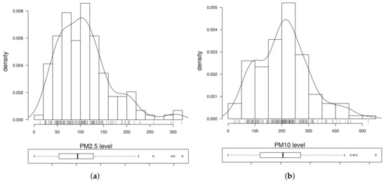
Figure 2.
Histogram for Chilean PM data using PM2.5 (a) and PM10 (b) levels recorded by the Pudahuel monitoring station in Santiago, Chile, during 2015.

Figure 3.
Scatterplot matrix for the listed covariates and response variables with Chilean PM data.
3.4. Parameter Estimation and Model Selection
In view of the exploratory analysis described previously, bivariate log-GBS distributions seem adequate to obtain the predictive model to be used in data-driven decision making when monitoring environmental pollution in Santiago. Then, the predictive bivariate regression model to be applied is given by
where is the log-response matrix and As mentioned, the parameters of the bivariate BS and BS-t models are estimated by the ML method, which has been implemented in the R software. A stepwise algorithm based on the BIC is used for variable selection within the set . The covariates were initially ordered according to the correlation with the response variables. Table 2 provides the results obtained by this variable selection algorithm for the bivariate BS regression model.
Table 2.
Results of the stepwise algorithm for the bivariate BS regression model and its corresponding BIC and log-likelihood values with Chilean PM data.
Next, parameter estimates (that is, the value that maximizes the log-likelihood function), estimated asymptotic SEs and p-values of the corresponding t-tests are obtained for each of the parameters of the bivariate BS regression model, where non-significant covariates were excluded at a 5% significance level. Its results are reported in Table 3, from where it is possible to note that the coefficients and should be removed when predicting ; however, both of them should be used when predicting . Further, coefficient should be removed when predicting , but considered when predicting .
Table 3.
ML estimate for listed parameter and corresponding estimated SE, p-value and maximized log-likelihood value for the BS model with Chilean PM data.
As mentioned, the MD can be considered to evaluate whether the proposed distributional assumption for the multivariate models is appropriate and also as a measure of global influence to identify multivariate outliers. In Figure 4a, an empirical probability versus theoretical probability (PP) plot is presented, with Kolmogorov-Smirnov (KS) acceptance regions at for transformed MDs. The KS test, although not particularly sensitive, but very competitive with other tests, is the only test that can be linked to a graphical tool as the PP plot. A graphical tool is always more desirable than a test due to its easier interpretation. However, if the graphical GOF tool can be accompanied by a p-value associated with a GOF test, it is more informative. This is the reason why we have used both GOF tools [56]. From the PP plot, the BS model does not have a good fit, which is corroborated by a p-value of 0.001 of the KS test associated with this PP plot. From Figure 4b, observe that cases appear as possible multivariate outliers in the BS model. These cases correspond to 10-June, 11-July, and 04-August of the year 2015, respectively.
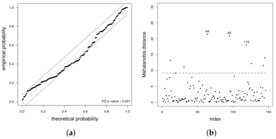
Figure 4.
PP plot with KS acceptance bands at 5% (a) and index plot for transformed Mahalanobis distance (MD) (b) using the BS model with Chilean PM data from the Pudahuel monitoring station, in Santiago, Chile, during 2015.
Next, we adopt a bivariate BS-t regression model to describe the data and apply the same variable selection algorithm as with the bivariate BS regression model, within the set ,, , , , , . An important point to consider under a t model is whether the degrees of freedom, , are estimated or not. Various authors [10,13,14,15,16,21] have worked on this issue and reported problems when estimating due to unboundedness and local maximum in the likelihood function. Thus, in order to overcome this difficulty, the parameter can be previously fixed or, otherwise, information for from the data can be obtained [14]. Then, to estimate the parameters of the bivariate BS-t regression model, we use the profiled log-likelihood function with fixed from 1 to 20. This procedure is known as the non-failing method and applied in each of the iterations of the stepwise algorithm, starting the procedure with and attaining an optimum at with the lowest BIC (113.1882); see Figure 5a. Table 4 provides the results obtained by this variable selection algorithm for the bivariate BS-t regression model.

Figure 5.
Profiled log-likelihood function with fixed from (a), PP plot with KS acceptance bands at (b), and index plot for transformed MD (c), using the BS-t model and Chilean PM data.
Table 4.
Results of the stepwise algorithm for the bivariate BS-t regression model and its corresponding BIC and log-likelihood values with Chilean PM data.
Next, parameter estimates, estimated asymptotic SEs and p-values of the corresponding t-tests are obtained for each of the parameters of the bivariate BS-t regression model, where non-significant covariates were excluded at a 5% significance level, in this case, . We use this level to obtain the BS-t model and its results are reported in Table 5. The BS-t model is proposed as optimal parsimonious, where the estimated is statistically significant and the coefficient must be discarded in the prediction of , but considered for .
Table 5.
ML estimate for the listed parameter and corresponding estimated SE, p-value and maximized log-likelihood value for the BS-t model and using Chilean PM data.
Figure 5b presents a PP plot with KS acceptance regions at 5% for transformed MDs. The plot shows that the bivariate BS-t model has a better fit than the BS model, with p-value of 0.8502 of the KS test. In addition, we fit the bivariate normal regression for comparison with an established model and summarize the BIC values of this model and of the bivariate BS and BS-t regression models in Table 6. Marginal normal regression models are less suitable than the bivariate normal regression model, as expected, with their BIC values omitted here. From Table 6 and Figure 5a, we confirm that the BS-t regression with degrees of freedom and the indicated covariates is the most adequate model for describing the Chilean PM data.
Table 6.
BIC and log-likelihood values with Chilean PM data for the indicated model.
3.5. Diagnostic Analytics
From Figure 5c, we can identify that cases appear as possible multivariate outliers in the BS-t model. These cases correspond to 10-June-2015 and 11-July-2015, respectively. As it is well known, outliers can or cannot be potentially influential cases, so that we now apply the local influence method for their evaluation.
In order to identify possible influential cases under the fitted model, diagnostic plots are presented for total local influence (). The schemes to be employed in this research are: (i) case-weight perturbation, (ii) correlation-matrix perturbation, (iii) response perturbation and (iv) a continuous covariate perturbation; see details about these schemes in [10]. Figure 6a–d present index plots for , , and under the case-weight perturbation scheme. For this scheme, we can distinguish that case appears as high potentially influential on in Figure 6a. In addition, this same case has a high potential influence only on in Figure 6c. Furthermore, in Figure 6b and in Figure 6d, there is no influence of this case on and , respectively. Figure 6e–h show index plots for , , and under the correlation matrix perturbation scheme. These figures indicate that under this perturbation scheme no cases stand out as high potentially influential considering the BS-t model. Figure 6i–l present index plots for , , and under the response variable perturbation scheme. From these figures, one can distinguish that case 74 has a high influence on PM10, when applying the BS-t regression model. Furthermore, case 74 also has some influence on for PM10, but not for and . Figure 6m–p present index plots for , , and under the covariate perturbation scheme. From these figures, we can observe that no cases appear as potentially influential cases in the bivariate BS-t model.
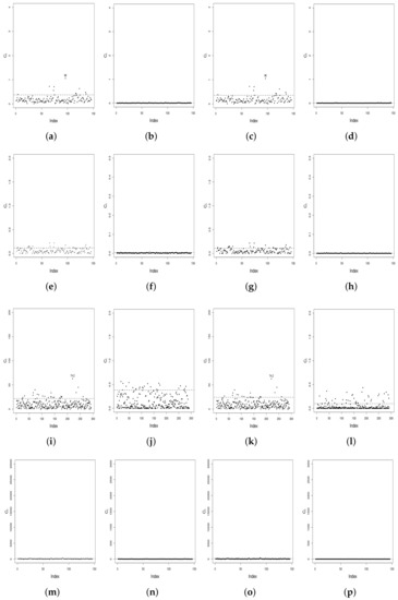
Figure 6.
Total local influence index plots of the BS-t model for (a,e,i,m), (b,f,j,n), (c,g,k,o) and (d,h,l,p) in (first row) case-weight perturbation; (second row) correlation matrix perturbation; (third row) response perturbation; and (fourth row) covariate perturbation, with Chilean PM data.
3.6. Analysis of Results
In summary, cases are identified as potentially influential data under the different perturbation schemes used, two of which cases are indicated also as possible outliers. These cases correspond to 10-June, 20-June, 11-July and 12-July of the year 2015, respectively. Case 64 (10-June-2015) was the day prior to the second highest PM2.5 level during the year, whereas case 74 (20-June-2015) was the day with the highest recorded level for PM2.5 and the second highest for PM10. Note that cases 95 and 96 (11-July-2015 and 12-July-2015) are 2 of 5 days with the largest measured rainfall (total precipitation) for the entire year, which might have also affected the low levels of PM2.5 and PM10 observed for case 96. Under these conditions, a much larger decrease was expected for PM levels than the predicted levels. Meteorological variables might affect the response variables in an indirect manner, as observed in the perturbation schemes.
Next, the prediction capacity of the bivariate BS-t regression model with respect to the primary quality guidelines for PM2.5 and PM10 is analyzed, based on which the degree of precision to detect critical episodes was determined. Table 7 provides the primary quality guidelines for PM2.5 and PM10 levels for 24 h.
Table 7.
Primary quality guidelines for PM2.5 and PM10 levels in 24 h [1,47].
The results for the corresponding predictive capacity of the BS-t model for the year 2015 are reported next. First, once again, observed versus predicted data during the 2015 CEM period for PM2.5 are analyzed. According to Figure 7, the model is capable of following the overall trend of the observed data. Nevertheless, just as for bivariate BS model, when an abrupt increase in the pollutant level is present from one day to another, it is not capable of predicting a value similar to the observed data. Note that cases presenting extreme residuals of low frequency in the histogram are those where large differences exist between the observed and predicted data. Table 8 contains the categorization of the observed and predicted measurements according to the primary air quality regulations of PM2.5 levels for the year 2015. Most underestimated cases occurs when the observed data are categorized as emergency.
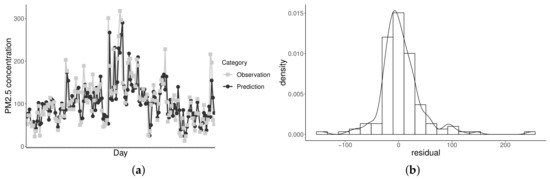
Figure 7.
Predicted versus observed PM2.5 levels (a) and residual histogram (b) for the BS-t model with Chilean PM data.
Table 8.
Categorization of observed and predicted PM2.5 levels according to air quality regulations during the CEM period for the Pudahuel monitoring station in Santiago, Chile, during 2015.
Just as for the PM2.5 level, a general underestimation of the PM10 level is noted. According to Figure 8, for extremely high measurements, a value similar to the observed data cannot be predicted by the model. Note that cases presenting extreme residuals of low frequency in the histogram are those where medium differences exist between the observed and predicted data. Table 9 contains the categorization of the observed and predicted measurements according to the primary air quality regulations for PM10 levels for the year 2015. Most of the underestimated cases occur when the observed data are categorized as “pre-emergency” or “emergency”.
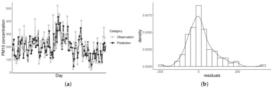
Figure 8.
Predicted versus observed PM10 levels (a) and residual histogram (b) for the BS-t model with Chilean PM data.
Table 9.
Categorization of observed and predicted PM10 levels according to air quality regulations during the CEM period for the Pudahuel monitoring station, in Santiago, Chile, during 2015.
4. Conclusions and Future Investigation
In this study, bivariate Birnbaum-Saunders log-linear models were fitted to predict the maximum PM2.5 and PM10 levels during critical episodes management in Santiago, Chile. The bivariate Birnbaum-Saunders-t model showed a better fit to the data and, consequently, more precise and robust results were obtained with respect to the Birnbaum-Saunders model. The proportion of accurate predictions about the corresponding observed categories, according to primary air quality regulations, was also better for the Birnbaum-Saunders-t model than for the Birnbaum-Saunders model, in both PM2.5 and PM10 levels. For the bivariate Birnbaum-Saunders model, statistically significant meteorological variables, at a 5% significance level, were: maximum level of PM2.5 of the present day, average wind speed of the present day, predicted temperature range for the next day, average relative humidity of the present day, total precipitation of the present day, average atmospheric pressure of the present day and the binary variable weekend/holiday. For the bivariate BS-t model, the statistically significant covariates, at a 5% significance level, were the same as those for the Birnbaum-Saunders model, except for total precipitation of the present day and average atmospheric pressure of the present day. The stepwise algorithm was used as a systematic variable selection tool to obtain the bivariate regression model based on the Bayesian information criterion. The Mahalanobis distance was employed to evaluate if the distributional assumption was appropriate for each model and also as global influence method to detect bivariate outliers. The local influence technique, under perturbation schemes of case-weight, correlation matrix, response variable and a continuous covariate, was utilized to identify possible influential cases under the fitted model. For the Birnbaum-Saunders-t model, predictions were superior for the maximum PM2.5 level than for the maximum PM10 level. Considering the categorization of PM2.5 estimates using the Birnbaum-Saunders-t model, it is worth mentioning that some alert and pre-emergency indications were overestimated in more relevant categories according to primary air quality regulations for PM2.5 levels. The regular, alert, pre-emergency and emergency categories obtained an 81.5%, 50.0%, 51.2% and 36.8% of assertiveness, respectively; see Table 8. For PM10 estimates using the Birnbaum-Saunders-t model, an 87.3% and 63.9% assertiveness were obtained for the regular and alert categories, while categorizations for pre-emergency and emergency were underestimated mainly under alert; see Table 8. Future research, which arose from the present applied investigation, is proposed as follows:
- (i)
- Incorporation in the modeling of temporal, spatial, functional and quantile regression structures, as well as measurement errors, and partial least squares, are suitable to be studied and can improve the predictive capability of the model [57,58,59,60,61,62,63].
- (ii)
- Traditional robust estimation methods as well as the theoretical study of quantitative robustness are also of interest [64].
- (iii)
- Other applications in the context of multivariate methods are in cluster analysis and principal component analysis, particularly when using principal components to remove the collinearity among covariates [65].
- (iv)
- An interesting field of application is in the statistical learning and neural networks.
The methodology used in this applied investigation provides options to explore other theoretical and numerical topics related, which are in progress and we hope to report them in other articles.
Author Contributions
Data curation, R.P., C.M.; formal analysis, C.M., V.L.; investigation, R.P., C.M., V.L., J.F.; methodology, R.P., C.M., V.L., J.F., F.R.; writing—original draft, R.P., C.M., V.L., J.F., F.R.; writing—review and editing, C.M., V.L. All authors have read and agreed to the published version of the manuscript.
Funding
This research was supported partially by project grants “Fondecyt 11190636” (C. Marchant) and “Fondecyt 1200525” (V. Leiva) from the National Agency for Research and Development (ANID) of the Chilean government and by ANID-Millennium Science Initiative Program—NCN17_059 (C. Marchant).
Institutional Review Board Statement
Not applicable.
Informed Consent Statement
Not applicable.
Data Availability Statement
Data and computational codes are available upon request from the authors.
Acknowledgments
The authors would also like to thank the editor and reviewers for their constructive comments which led to improve the presentation of the manuscript.
Conflicts of Interest
The authors declare no conflict of interest.
References
- MMA. Establishment of Primary Quality Guideline for Inhalable Fine Particulate Matter PM2.5; Technical Report Decree 12; Ministry of Environment of the Chilean Government: Santiago, Chile, 2011.
- Stanek, L.; Sacks, J.; Dutton, S.; Dubois, J. Attributing health effects to apportioned components and sources of particulate matter: An evaluation of collective results. Atmos. Environ. 2011, 45, 5655–5663. [Google Scholar] [CrossRef]
- Cakmak, S.; Dales, R.E.; Vidal, C.B. Air pollution and hospitalization for epilepsy in Chile. Environ. Int. 2010, 36, 501–505. [Google Scholar] [CrossRef]
- Ostro, P. Air Pollution and Its Impacts on Health in Santiago, Chile; Earthscan: London, UK, 2003. [Google Scholar]
- Kinney, P.L. Climate change, air quality, and human health. Am. J. Prev. Med. 2008, 35, 459–467. [Google Scholar] [CrossRef] [PubMed]
- Marchant, C.; Leiva, V.; Cavieres, M.F.; Sanhueza, A. Air contaminant statistical distributions with application to PM10 in Santiago, Chile. Rev. Environ. Contam. Toxicol. 2013, 223, 1–31. [Google Scholar] [PubMed]
- Cavieres, M.F.; Leiva, V.; Marchant, C.; Rojas, F. A methodology for data-driven decision making in the monitoring of particulate matter environmental contamination in Santiago of Chile. Rev. Environ. Contam. Toxicol. 2020, in press. Available online: https://doi.org/10.1007/398_2020_41 (accessed on 22 January 2021).
- Clements, N.; Hannigan, M.; Miller, S.; Peel, J.; Milford, J. Comparisons of urban and rural PM10−2.5 and PM2.5 mass levels and semi-volatile fractions in northeastern Colorado. Atmos. Chem. Phys. 2016, 16, 7469–7484. [Google Scholar] [CrossRef]
- Desai, U.; Watson, A. Associations between ultrafine particles and co-pollutant levels in the Tampa Bay Area. J. Environ. Health 2016, 78, 14–21. [Google Scholar]
- Marchant, C.; Leiva, V.; Cysneiros, F.J.A.; Vivanco, J.F. Diagnostics in multivariate generalized Birnbaum-Saunders regression models. J. Appl. Stat. 2016, 43, 2829–2849. [Google Scholar] [CrossRef]
- Marchant, C.; Leiva, V.; Christakos, G.; Cavieres, M.F. Monitoring urban environmental pollution by bivariate control charts: New methodology and case study in Santiago, Chile. Environmetrics 2019, 30, e2551. [Google Scholar] [CrossRef]
- Marchant, C.; Leiva, V.; Cysneiros, F.J.A. A multivariate log-linear model for Birnbaum-Saunders distributions. IEEE Trans. Reliab. 2016, 65, 816–827. [Google Scholar] [CrossRef]
- Paula, G.A.; Leiva, V.; Barros, M.; Liu, S. Robust statistical modeling using the Birnbaum-Saunders-t distribution applied to insurance. Appl. Stoch. Model. Bus. Ind. 2021, 28, 16–34. [Google Scholar] [CrossRef]
- Athayde, E.; Azevedo, A.; Barros, M.; Leiva, V. Failure rate of Birnbaum-Saunders distributions: Shape, change-point, estimation and robustness. Braz. J. Probab. Stat. 2019, 33, 301–328. [Google Scholar] [CrossRef]
- Lange, K.L.; Little, J.A.; Taylor, M.G.J. Robust statistical modeling using the t distribution. J. Am. Stat. Assoc. 1989, 84, 881–896. [Google Scholar] [CrossRef]
- Lucas, A. Robustness of the student t based M-estimator. Commun. Stat. Theory Methods 1997, 26, 1165–1182. [Google Scholar] [CrossRef]
- Montgomery, D.C.; Peck, E.A.; Vining, G.G. Introduction to Linear Regression Analysis; Wiley: New York, NY, USA, 2012. [Google Scholar]
- Sanhueza, A.; Sen, P.K.; Leiva, V. A robust procedure in nonlinear models for repeated measurements. Commun. Stat. Theory Methods 2009, 38, 138–155. [Google Scholar] [CrossRef]
- Leiva, V.; Sanhueza, A.; Sen, P.K.; Araneda, N. M-procedures in the general multivariate nonlinear regression model. Pak. J. Stat. 2010, 26, 1–13. [Google Scholar]
- Agullo, J.; Croux, C.; Van Aelst, S. The multivariate least-trimmed squares estimator. J. Multivar. Anal. 2008, 99, 311–338. [Google Scholar] [CrossRef]
- Marchant, C.; Leiva, V.; Cysneiros, F.J.A.; Liu, S. Robust multivariate control charts based on Birnbaum-Saunders distributions. J. Stat. Comput. Simul. 2018, 88, 182–202. [Google Scholar] [CrossRef]
- Becker, C.; Gather, U. The masking breakdown point of multivariate outlier identification rules. J. Am. Stat. Assoc. 1999, 94, 947–955. [Google Scholar] [CrossRef]
- Jobe, J.M.; Pokojovy, M. A cluster-based outlier detection scheme for multivariate data. J. Am. Stat. Assoc. 2015, 110, 543–1551. [Google Scholar] [CrossRef]
- Aykroyd, R.G.; Leiva, V.; Marchant, C. Multivariate Birnbaum-Saunders distributions: Modelling and applications. Risks 2018, 6, 21. [Google Scholar] [CrossRef]
- Wilkinson, L. Visualizing big data outliers through distributed aggregation. IEEE Trans. Vis. Comput. Graph. 2017, 24, 256–266. [Google Scholar] [CrossRef]
- Talagala, P.D.; Hyndman, R.J.; Smith-Miles, K. Anomaly detection in high-dimensional data. J. Comput. Graph. Stat. 2021, in press. [Google Scholar] [CrossRef]
- Ro, K.; Zou, C.; Wang, Z.; Yin, G. Outlier detection for high-dimensional data. Biometrika 2015, 102, 589–599. [Google Scholar] [CrossRef]
- Rieck, J.; Nedelman, J. A log-linear model for the Birnbaum-Saunders distribution. Technometrics 1991, 3, 51–60. [Google Scholar]
- Dasilva, A.; Dias, R.; Leiva, V.; Marchant, C.; Saulo, H. Birnbaum-Saunders regression models: A comparative evaluation of three approaches. J. Stat. Comput. Simul. 2020, 90, 2552–2570. [Google Scholar] [CrossRef]
- Kundu, D.; Balakrishnan, N.; Jamalizadeh, A. Bivariate Birnbaum-Saunders distribution and associated inference. J. Multivar. Anal. 2010, 101, 113–125. [Google Scholar] [CrossRef]
- Leiva, V.; Aykroyd, R.G.; Marchant, C. Discussion of “Birnbaum-Saunders distribution: A review of models, analysis, and applications” and a novel multivariate data analytics for an economics example in the textile industry. Appl. Stoch. Model. Bus. Ind. 2019, 35, 112–117. [Google Scholar] [CrossRef]
- Garcia-Papani, F.; Uribe-Opazo, M.A.; Leiva, V.; Aykroyd, R.G. Birnbaum-Saunders spatial modelling and diagnostics applied to agricultural engineering data. Stoch. Environ. Res. Risk Assess. 2017, 31, 105–124. [Google Scholar] [CrossRef]
- Garcia-Papani, F.; Leiva, V.; Ruggeri, F.; Uribe-Opazo, M.A. Kriging with external drift in a Birnbaum-Saunders geostatistical model. Stoch. Environ. Res. Risk Assess. 2018, 32, 1517–1530. [Google Scholar] [CrossRef]
- Leiva, V.; Marchant, C.; Ruggeri, F.; Saulo, H. A criterion for environmental assessment using Birnbaum-Saunders attribute control charts. Environmetrics 2015, 26, 463–476. [Google Scholar] [CrossRef]
- Leiva, V.; Ferreira, M.; Gomes, M.I.; Lillo, C. Extreme value Birnbaum-Saunders regression models applied to environmental data. Stoch. Environ. Res. Risk Assess. 2016, 30, 1045–1058. [Google Scholar] [CrossRef]
- Leiva, V.; Sánchez, L.; Galea, M.; Saulo, H. Global and local diagnostic analytics for a geostatistical model based on a new approach to quantile regression. Stoch. Environ. Res. Risk Assess. 2020, 34, 1457–1471. [Google Scholar] [CrossRef]
- Leiva, V.; Saulo, H.; Souza, R.; Aykroyd, R.G.; Vila, R. A new BISARMA time series model for forecasting mortality using weather and particulate matter data. J. Forecast. 2021, 40, 346–364. [Google Scholar] [CrossRef]
- Martinez, S.; Giraldo, R.; Leiva, V. Birnbaum-Saunders functional regression models for spatial data. Stoch. Environ. Res. Risk Assess. 2019, 33, 1765–1780. [Google Scholar] [CrossRef]
- Rocha, S.S.; Espinheira, P.L.; Cribari-Neto, F. Residual and local influence analyses for unit gamma regressions. Stat. Neerl. 2021, in press. [Google Scholar] [CrossRef]
- R Core Team. R: A Language and Environment for Statistical Computing; R Foundation for Statistical Computing: Vienna, Austria, 2020. [Google Scholar]
- Lange, K. Numerical Analysis for Statisticians; Springer: New York, NY, USA, 2001. [Google Scholar]
- Lesaffre, E.; Verbeke, G. Local influence in linear mixed models. Biometrics 1998, 54, 570–582. [Google Scholar] [CrossRef]
- Verbeke, G.; Molenberghs, G. Linear Mixed Models for Longitudinal Data; Springer: New York, NY, USA, 2000. [Google Scholar]
- Troncoso, R.; de Grange, L.; Cifuentes, L. Effects of environmental alerts and pre-emergencies on pollutant levels in Santiago, Chile. Atmos. Environ. 2012, 61, 550–557. [Google Scholar] [CrossRef]
- Cakmak, S.; Dales, R.; Gultekin, T.; Vidal, C.; Fernandez, M.; Rubio, M.; Oyola, P. Components of Particulate Air Pollution and Emergency Department Visits in Chile. Arch. Environ. Occup. Health 2009, 64, 148–155. [Google Scholar] [CrossRef] [PubMed]
- Yáñez, M.; Baettig, R.; Cornejo, J.; Zamudio, F.; Guajardo, J.; Fica, R. Urban airborne matter in central and southern Chile: Effects of meteorological conditions on fine and coarse particulate matter. Atmos. Environ. 2017, 161, 221–234. [Google Scholar] [CrossRef]
- CONAMA. Establishment of Primary Quality Guideline for PM10 that Regulates Environmental Alerts; Technical Report Decree 59; Ministry of Environment (CONAMA) of the Chilean Government: Santiago, Chile, 1998.
- Morales, R.G.; Llanos, A.; Merino, M.; Gonzalez-Rojas, C.H. A semi-empirical method of PM10 atmospheric pollution forecast at Santiago. Nat. Environ. Pollut. Technol. 2012, 11, 181–186. [Google Scholar]
- Cassmassi 2.0. Internet. 2017. Available online: http://www.forexconmql.cl/geos/pics5/Cassmassi2.htm (accessed on 28 February 2021).
- MMA. Approval of a New Form to Implement an Air Quality Forecast Methodology for Particulate Matter PM10 in the Metropolitan Region; Resolution 10.047; Ministry of Environment of the Chilean Government: Santiago, Chile, 2000.
- Saide, P.E.; Mena-Carrasco, M.; Tolvett, S.; Hernandez, P.; Carmichael, G.R. Air quality forecasting for winter-time PM2.5 episodes occurring in multiple cities in central and southern Chile. J. Geophys. Res. Atmos. 2016, 121, 558–575. [Google Scholar] [CrossRef]
- MMA. Approval of an Air Quality Forecast Methodology for Particulate Matter PM2.5, to Use in Decontamination Programs that Apply; Resolution 355; Ministry of Environment Chilean Government: Santiago, Chile, 2016.
- Alvarado, S.; Silva, C.; Cáceres, D. Critical Episodes of PM10 Particulate Matter Pollution in Santiago of Chile, an Approximation Using Two Prediction Methods: MARS Models and Gamma Models. In Air Pollution; Mukesh, K., Ed.; IntechOpen: Rijeka, Croatia, 2012. [Google Scholar]
- MMA. Establishes a Prevention and Atmospheric Decontamination Plan for the Santiago Metropolitan Region; Technical Report Decree 31; Ministry of Environment of the Chilean Government: Santiago, Chile, 2017.
- Cysneiros, F.J.A.; Leiva, V.; Liu, S.; Marchant, C.; Scalco, P. A Cobb-Douglas type model with stochastic restrictions: Formulation, local influence diagnostics and data analytics in economics. Qual. Quant. 2019, 53, 1693–1719. [Google Scholar] [CrossRef]
- Castro-Kuriss, C.; Huerta, M.; Leiva, V.; Tapia, A. On some goodness-of-fit tests and their connection to graphical methods with uncensored and censored data. In Management Science and Engineering Management; Xu, J., Ahmed, S.E., Duca, G., Cooke, F.L., Eds.; Springer: Berlin, Germany, 2020; pp. 157–183. [Google Scholar]
- Leiva, V.; Saulo, H.; Leao, J.; Marchant, C. A family of autoregressive conditional duration models applied to financial data. Comput. Stat. Data Anal. 2014, 79, 175–191. [Google Scholar] [CrossRef]
- Huerta, M.; Leiva, V.; Liu, S.; Rodriguez, M.; Villegas, D. On a partial least squares regression model for asymmetric data with a chemical application in mining. Chemom. Intell. Lab. Syst. 2019, 190, 55–68. [Google Scholar] [CrossRef]
- Chahuan-Jimenez, K.; Rubilar, R.; de la Fuente-Mella, H.; Leiva, V. Breakpoint analysis for the COVID-19 pandemic and its effect on the stock markets. Entropy 2021, 23, 100. [Google Scholar] [CrossRef]
- Carrasco, J.M.F.; Figueroa-Zúñiga, J.; Leiva, V.; Riquelme, M.; Aykroyd, R.G. An errors-in-variables model based on the Birnbaum-Saunders the distribution and its diagnostics with an application to earthquake data. Stoch. Environ. Res. Risk Assess. 2020, 34, 369–380. [Google Scholar] [CrossRef]
- Santos-Neto, M.; Cysneiros, F.J.A.; Leiva, V.; Barros, M. Reparameterized Birnbaum-Saunders regression models with varying precision. Electron. J. Stat. 2016, 10, 2825–2855. [Google Scholar] [CrossRef]
- Giraldo, R.; Herrera, L.; Leiva, V. Cokriging prediction using as secondary variable a functional random field with application in environmental pollution. Mathematics 2020, 8, 1305. [Google Scholar] [CrossRef]
- Sánchez, L.; Leiva, V.; Galea, M.; Saulo, H. Birnbaum-Saunders quantile regression and its diagnostics with application to economic data. Appl. Stoch. Model. Bus. Ind. 2021, 37, 53–73. [Google Scholar] [CrossRef]
- Velasco, H.; Laniado, H.; Toro, M.; Leiva, V.; Lio, Y. Robust three-step regression based on comedian and its performance in cell-wise and case-wise outliers. Mathematics 2020, 8, 1259. [Google Scholar] [CrossRef]
- Ramirez-Figueroa, J.A.; Martin-Barreiro, C.; Nieto, A.B.; Leiva, V.; Galindo, M.P. A new principal component analysis by particle swarm optimization with an environmental application for data science. Stoch. Environ. Res. Risk Assess. 2021, in press. [Google Scholar] [CrossRef]


Publisher’s Note: MDPI stays neutral with regard to jurisdictional claims in published maps and institutional affiliations. |
© 2021 by the authors. Licensee MDPI, Basel, Switzerland. This article is an open access article distributed under the terms and conditions of the Creative Commons Attribution (CC BY) license (http://creativecommons.org/licenses/by/4.0/).