N-Fold Darboux Transformation for the Classical Three-Component Nonlinear Schrödinger Equations and Its Exact Solutions

Abstract

In this paper, by using the gauge transformation and the Lax pairs, the N-fold Darboux transformation (DT) of the classical three-component nonlinear Schrödinger (NLS) equations is given. In addition, by taking seed solutions and using the DT, exact solutions for the given NLS equations are constructed.

1. Introduction

Darboux transformation (DT) is an important technique to construct exact solutions of nonlinear partial differential equations [1]. The main significance of the DT is that infinite sequences of solutions to nonlinear equations can be generated by algebraic procedures. Thus, it has attracted much attention from physicists and mathematicians, it is now playing an important role in mechanics, physics, and differential geometry. The DT for the KdV equation, sine-Gordon equation, and nonlinear Schrödinger (NLS) equations, etc, were widely studied and many great scientific achievements have been derived [2,3,4,5,6,7].

The NLS equation is widely used in physics [8,9,10,11,12,13,14,15], nonlinear optics [16,17], and soft condensed matter physics [18] and there has been a vast amount of literature involving the NLS equation over the years. The applications of the DT in higher multicomponent NLS equations spatial dimensions and nonlocal equations have attracted much attention over the years [19,20,21,22]. Recently there has been an additional interest that has caused a hot topic of research, mainly due to Mark J. Ablowitz and Ziad H. Musslimani developed the nonlocal NLS equations [23,24]. In [25], Zhenya Yan introduced a new integrable nonlocal general vector NLS equation and found its exact solutions (See many other interesting examples about nonlocal NLS equations in [26,27,28,29] ).

In [30], the classical three-component NLS equations belong to the category of evolutionary equations, for the solution of which the method of the inverse scattering problem is successfully applied.

The rest of the paper is organized as follows: In Section 2, we construct the DT for the three-component NLS equations and give the 1- and 2-fold exact solutions for the three-component NLS equations. In Section 3, we give some conclusions.

2. Darboux Transformation and Exact Solutions for the NLS Equations

2.1. Darboux Transformation

Let $n\in N$, $I_n$ denote the identity matrix of size; n, ${\alpha }_1$ and ${\alpha }_2$ are different constants. The matrix spectral problems of the NLS equations read [30]

$${\varphi }_x=\mathbf{U}\varphi =\mathbf{U}(u,\lambda )\varphi ,{\varphi }_t=\mathbf{V}\varphi =\mathbf{V}(u,\lambda )\varphi ,$$

(1)

with the Lax pairs as follows:

$$\mathbf{U}=i(\lambda \mathsf{\Psi }+D),\mathbf{V}=i({\lambda }^2\mathsf{{\rm Y}}+G).$$

(2)

The four matrices $\mathsf{\Psi }$, $\mathsf{{\rm Y}}$, D and G as follows:

$$\mathsf{\Psi }=diag({\alpha }_1,{\alpha }_2{I}_n),D=D\left(u\right)=P=\left(\begin{array}{cc}0& p\\ q& 0\end{array}\right),$$

(3)

$$\mathsf{{\rm Y}}=diag({\beta }_1,{\beta }_2{I}_n),$$

(4)

$$G=G(u,\lambda )=\frac{\beta }{\alpha }\lambda \left(\begin{array}{cc}0& p\\ q& 0\end{array}\right)-\frac{\beta }{{\alpha }^2}\left(\begin{array}{cc}pq& i{p}_x\\ -i{q}_x& -pq\end{array}\right),$$

(5)

where $p=(p_1,p_2,\cdots ,p_n)$, $q={(q_1,q_2,\cdots ,q_n)}^T$, $u={(p,q^T)}^T$, and ${\beta }_1$ and ${\beta }_2$ are different constants. Note that G can be given by using the potential matrix D as follows:

$$G=\frac{\beta }{\alpha }\lambda D-\frac{\beta }{{\alpha }^2}\left(\begin{array}{cc}1& 0\\ 0& -I_n\end{array}\right)D^2-\frac{\beta }{{\alpha }^2}\left(\begin{array}{cc}i& 0\\ 0& -i{I}_n\end{array}\right)D_x.$$

(6)

when $p_j=q_j=0$, $2\le j\le n$, the spectral problem in (1) becomes the standard AKNS spectral problem [31].

Now, we consider the system as follows [30]:

$$\left\{\begin{array}{c}{p}_{1,t}(x,t)=\frac{1}{2}i[p_{1,xx}+2\left(\right|p_1{|}^2+|p_2{|}^2+|p_3{|}^2\left)p_1\right],\hfill \\ p_{2,t}(x,t)=\frac{1}{2}i[p_{2,xx}+2\left(\right|p_1{|}^2+|p_2{|}^2+|p_3{|}^2\left)p_2\right],\hfill \\ p_{3,t}(x,t)=\frac{1}{2}i[p_{3,xx}+2\left(\right|p_1{|}^2+|p_2{|}^2+|p_3{|}^2\left)p_3\right],\hfill \end{array}\right.$$

(7)

where $p_j(x,t)$$(1\le j\le 3)$ are complex valued functions of the real variables x and t. From Equations (2), (3) and (6), we obtain the following spectral problem. Firstly, the corresponding cospectral problems for Equation (7) are introduced

$${\varphi }_x=\mathbf{U}\varphi ,{\varphi }_t=\mathbf{V}\varphi ,\varphi ={({\varphi }_1,{\varphi }_2,{\varphi }_3,{\varphi }_4)}^T.$$

(8)

where $\mathbf{U}$ and $\mathbf{V}$ are [32,33,34,35]:

$$\mathbf{U}=\left(\begin{array}{cccc}-i\lambda & i{p}_1& i{p}_2& i{p}_3\\ i{p}_1^{*}& i\lambda & 0& 0\\ i{p}_2^{*}& 0& i\lambda & 0\\ i{p}_3^{*}& 0& 0& i\lambda \end{array}\right),$$

(9)

$$\mathbf{V}=\left(\begin{array}{cccc}-i{\lambda }^2+\frac{i}{2}\left(\right|p_1{|}^2+|p_2{|}^2+|p_3{|}^2)& i\lambda p_1-\frac{1}{2}{p}_{1,x}& i\lambda p_2-\frac{1}{2}{p}_{2,x}& i\lambda p_3-\frac{1}{2}{p}_{3,x}\\ i\lambda p_1^{*}+\frac{1}{2}{p}_{1,x}^{*}& i{\lambda }^2-\frac{i}{2}{\left|p_1\right|}^2& -\frac{i}{2}{p}_2{p}_1^{*}& -\frac{i}{2}{p}_3{p}_1^{*}\\ i\lambda p_2^{*}+\frac{1}{2}{p}_{2,x}^{*}& -\frac{i}{2}{p}_1{p}_2^{*}& i{\lambda }^2-\frac{i}{2}{\left|p_2\right|}^2& -\frac{i}{2}{p}_3{p}_2^{*}\\ i\lambda p_3^{*}+\frac{1}{2}{p}_{3,x}^{*}& -\frac{i}{2}{p}_1{p}_3^{*}& -\frac{i}{2}{p}_2{p}_3^{*}& i{\lambda }^2-\frac{i}{2}{\left|p_3\right|}^2\end{array}\right),$$

(10)

here $\lambda$ is a spectral parameter, $\varphi ={({\varphi }_1,{\varphi }_2,{\varphi }_3,{\varphi }_4)}^T$ is a column vector solution of Equations (9) and (10) associated with an eigenvalue $\lambda$.

We introduce a gauge transformation T [36] of Equations (9) and (10), where

$${\tilde{\varphi }}_n=T{\varphi }_n.$$

(11)

Now, let us define T as follows:

$$T=\left(\begin{array}{cccc}{T}_{11}\left(\lambda \right)& T_{12}\left(\lambda \right)& T_{13}\left(\lambda \right)& T_{14}\left(\lambda \right)\\ T_{21}\left(\lambda \right)& T_{22}\left(\lambda \right)& T_{23}\left(\lambda \right)& T_{24}\left(\lambda \right)\\ T_{31}\left(\lambda \right)& T_{32}\left(\lambda \right)& T_{33}\left(\lambda \right)& T_{34}\left(\lambda \right)\\ T_{41}\left(\lambda \right)& T_{42}\left(\lambda \right)& T_{43}\left(\lambda \right)& T_{44}\left(\lambda \right)\end{array}\right),$$

(12)

$$\widetilde{{\varphi }_x}=\tilde{\mathbf{U}}\tilde{\varphi },\tilde{\mathbf{U}}=(T_x+T\mathbf{U})T^{-1},$$

(13)

$$\widetilde{{\varphi }_t}=\tilde{\mathbf{V}}\tilde{\varphi },\tilde{\mathbf{V}}=(T_t+T\mathbf{V})T^{-1}.$$

(14)

If the $\tilde{\mathbf{U}}$, $\tilde{\mathbf{V}}$ and $\mathbf{U}$, $\mathbf{V}$ have the same types, system (10) and (11) are called DT of Equation (7) [26].

Let $\psi ={({\psi }_1,{\psi }_2,{\psi }_3,{\psi }_4)}^T$, $\phi ={({\phi }_1,{\phi }_2,{\phi }_3,{\phi }_4)}^T$, $X={(X_1,X_2,X_3,X_4)}^T$ and $Y={(Y_1,Y_2,Y_3,Y_4)}^T$ be four basic solutions of systems (9) and (10), then we give the following linear algebraic systems [19,20]:

$$\left\{\begin{array}{c}\sum _{i=0}^{N-1}(A_{11}^{\left(i\right)}+A_{12}^{\left(i\right)}{M}_j^{\left(1\right)}+A_{13}^{\left(i\right)}{M}_j^{\left(2\right)}+A_{14}^{\left(i\right)}{M}_j^{\left(3\right)}){\lambda }_j^i=-{\lambda }_j^N,\hfill \\ \sum _{i=0}^{N-1}(A_{21}^{\left(i\right)}+A_{22}^{\left(i\right)}{M}_j^{\left(1\right)}+A_{23}^{\left(i\right)}{M}_j^{\left(2\right)}+A_{24}^{\left(i\right)}{M}_j^{\left(3\right)}){\lambda }_j^i=-M_j^{\left(1\right)}{\lambda }_j^N,\hfill \\ \sum _{i=0}^{N-1}(A_{31}^{\left(i\right)}+A_{32}^{\left(i\right)}{M}_j^{\left(1\right)}+A_{33}^{\left(i\right)}{M}_j^{\left(2\right)}+A_{34}^{\left(i\right)}{M}_j^{\left(3\right)}){\lambda }_j^i=-M_j^{\left(2\right)}{\lambda }_j^N,\hfill \\ \sum _{i=0}^{N-1}(A_{41}^{\left(i\right)}+A_{42}^{\left(i\right)}{M}_j^{\left(1\right)}+A_{43}^{\left(i\right)}{M}_j^{\left(2\right)}+A_{44}^{\left(i\right)}{M}_j^{\left(3\right)}){\lambda }_j^i=-M_j^{\left(3\right)}{\lambda }_j^N,\hfill \end{array}\right.$$

(15)

with

$$\left\{\begin{array}{c}{M}_j^{\left(1\right)}=\frac{{\psi }_2+v_j^{\left(1\right)}{\phi }_2+v_j^{\left(2\right)}{X}_2+v_j^{\left(3\right)}{Y}_2}{{\psi }_1+v_j^{\left(1\right)}{\phi }_1+v_j^{\left(2\right)}{X}_1+v_j^{\left(3\right)}{Y}_1},\hfill \\ M_j^{\left(2\right)}=\frac{{\psi }_3+v_j^{\left(1\right)}{\phi }_3+v_j^{\left(2\right)}{X}_3+v_j^{\left(3\right)}{Y}_3}{{\psi }_1+v_j^{\left(1\right)}{\phi }_1+v_j^{\left(2\right)}{X}_1+v_j^{\left(3\right)}{Y}_1},\hfill \\ M_j^{\left(3\right)}=\frac{{\psi }_4+v_j^{\left(1\right)}{\phi }_4+v_j^{\left(2\right)}{X}_4+v_j^{\left(3\right)}{Y}_4}{{\psi }_1+v_j^{\left(1\right)}{\phi }_1+v_j^{\left(2\right)}{X}_1+v_j^{\left(3\right)}{Y}_1},0\le j\le 4N,\hfill \end{array}\right.$$

(16)

where ${\lambda }_j$ and $v_j^{\left(k\right)}$, $(i\ne k,{\lambda }_i\ne {\lambda }_j,v_i^{\left(k\right)}\ne v_j^{\left(k\right)},k=1,2,3)$ should be appropriate parameters. Thus, the determinants of coefficients for Equation (15) are nonzero.

From Equation (12), we can define a $4\times 4$ matrix T as

$$\left\{\begin{array}{c}{T}_{11}={\lambda }^N+\sum _{i=0}^{N-1}{A}_{11}^{\left(i\right)}{\lambda }^i,T_{12}=\sum _{i=0}^{N-1}{A}_{12}^{\left(i\right)}{\lambda }^i,T_{13}=\sum _{i=0}^{N-1}{A}_{13}^{\left(i\right)}{\lambda }^i,\hfill \\ T_{14}=\sum _{i=0}^{N-1}{A}_{14}^{\left(i\right)}{\lambda }^i,T_{21}=\sum _{i=0}^{N-1}{A}_{21}^{\left(i\right)}{\lambda }^i,T_{22}={\lambda }^N+\sum _{i=0}^{N-1}{A}_{22}^{\left(i\right)}{\lambda }^i,\hfill \\ T_{23}=\sum _{i=0}^{N-1}{A}_{23}^{\left(i\right)}{\lambda }^i,T_{24}=\sum _{i=0}^{N-1}{A}_{24}^{\left(i\right)}{\lambda }^i,T_{31}=\sum _{i=0}^{N-1}{A}_{31}^{\left(i\right)}{\lambda }^i,\hfill \\ T_{32}=\sum _{i=0}^{N-1}{A}_{32}^{\left(i\right)}{\lambda }^i,T_{33}={\lambda }^N+\sum _{i=0}^{N-1}{A}_{33}^{\left(i\right)}{\lambda }^i,T_{34}=\sum _{i=0}^{N-1}{A}_{34}^{\left(i\right)}{\lambda }^i,\hfill \\ T_{41}=\sum _{i=0}^{N-1}{A}_{41}^{\left(i\right)}{\lambda }^i,T_{42}=\sum _{i=0}^{N-1}{A}_{42}^{\left(i\right)}{\lambda }^i,\hfill \\ T_{43}=\sum _{i=0}^{N-1}{A}_{43}^{\left(i\right)}{\lambda }^i,T_{44}={\lambda }^N+\sum _{i=0}^{N-1}{A}_{44}^{\left(i\right)}{\lambda }^i,\hfill \end{array}\right.$$

(17)

where N is natural number, and the $A_{mn}^{\left(i\right)}$ ($m,n=1,2,3,4$, $i\ge 0$ ) are the functions of x and t. Through calculations, we obtain T as following:

$$\Delta T={\mathsf{\Pi }}_{j=1}^{4N}(\lambda -{\lambda }_j),$$

(18)

which proves that ${\lambda }_j(1\le j\le 4N)$ are $4N$ roots of T. Based on Equation (18), we will prove that $\tilde{\mathbf{U}}$ and $\tilde{\mathbf{V}}$ have the same forms with $\mathbf{U}$ and $\mathbf{V}$ respectively.

Proposition 1. 

The matrix $\tilde{\mathbf{U}}$ defined by Equation (9) has the same type as $\mathbf{U}$, i.e.,

$$\tilde{\mathbf{U}}=\left(\begin{array}{cccc}-i\lambda & i\widetilde{p_1}& i\widetilde{p_2}& i\widetilde{p_3}\\ i\widetilde{p_1^{*}}& i\lambda & 0& 0\\ i\widetilde{p_2^{*}}& 0& i\lambda & 0\\ i\widetilde{p_3^{*}}& 0& 0& i\lambda \end{array}\right).$$

(19)

The transformation between old and new potentials are shown by the following formulas:

$$\left\{\begin{array}{c}\widetilde{p_1}(x,t)=p_1(x,t)+2A_{12},\hfill \\ \widetilde{p_2}(x,t)=p_2(x,t)+2A_{13},\hfill \\ \widetilde{p_3}(x,t)=p_3(x,t)+2A_{14}.\hfill \end{array}\right.$$

(20)

The transformations (20) are used to get a DT of the spectral problem (13).

Proof. 

Let $T^{-1}=\frac{T^{*}}{\Delta T}$ with

$$(T_x+T\mathbf{U})T^{*}=\left(\begin{array}{cccc}{\mathcal{B}}_{11}\left(\lambda \right)& {\mathcal{B}}_{12}\left(\lambda \right)& {\mathcal{B}}_{13}\left(\lambda \right)& {\mathcal{B}}_{14}\left(\lambda \right)\\ {\mathcal{B}}_{21}\left(\lambda \right)& {\mathcal{B}}_{22}\left(\lambda \right)& {\mathcal{B}}_{23}\left(\lambda \right)& {\mathcal{B}}_{24}\left(\lambda \right)\\ {\mathcal{B}}_{31}\left(\lambda \right)& {\mathcal{B}}_{32}\left(\lambda \right)& {\mathcal{B}}_{33}\left(\lambda \right)& {\mathcal{B}}_{34}\left(\lambda \right)\\ {\mathcal{B}}_{41}\left(\lambda \right)& {\mathcal{B}}_{42}\left(\lambda \right)& {\mathcal{B}}_{43}\left(\lambda \right)& {\mathcal{B}}_{44}\left(\lambda \right)\end{array}\right).$$

(21)

It is easy to verify that ${\mathcal{B}}_{s,l}(1\le s,l\le 4)$ are $4N$ -order or $(4N+1)$ -order polynomial in $\lambda$. □

Through some accurate calculations, ${\lambda }_j(1\le j\le 4)$ are the roots of ${\mathcal{B}}_{s,l}(1\le s,l\le 4)$. Thus, Equation (21) has the following structure

$$(T_x+T\mathbf{U})T^{*}=(\Delta T)\mathcal{C}\left(\lambda \right),$$

(22)

where

$$\mathcal{C}\left(\lambda \right)=\left(\begin{array}{cccc}{\mathcal{C}}_{11}^{\left(1\right)}\lambda +{\mathcal{C}}_{11}^{\left(0\right)}& {\mathcal{C}}_{12}^{\left(0\right)}& {\mathcal{C}}_{13}^{\left(0\right)}& {\mathcal{C}}_{14}^{\left(0\right)}\\ {\mathcal{C}}_{21}^{\left(0\right)}& {\mathcal{C}}_{22}^{\left(1\right)}\lambda +{\mathcal{C}}_{22}^{\left(0\right)}& {\mathcal{C}}_{23}^{\left(0\right)}& {\mathcal{C}}_{24}^{\left(0\right)}\\ {\mathcal{C}}_{31}^{\left(0\right)}& {\mathcal{C}}_{32}^{\left(0\right)}& {\mathcal{C}}_{33}^{\left(1\right)}\lambda +{\mathcal{C}}_{33}^{\left(0\right)}& {\mathcal{C}}_{34}^{\left(0\right)}\\ {\mathcal{C}}_{41}^{\left(0\right)}& {\mathcal{C}}_{42}^{\left(0\right)}& {\mathcal{C}}_{43}^{\left(0\right)}& {\mathcal{C}}_{44}^{\left(1\right)}\lambda +{\mathcal{C}}_{44}^{\left(0\right)}\end{array}\right),$$

(23)

and ${\mathcal{C}}_{mn}^{\left(k\right)}($ m,n $=1,2,3,4,$ k $= 0,1)$ satisfy the functions without $\lambda$. Then Equation (22) can be rewritten as

$$(T_x+T\mathbf{U})=\mathcal{C}\left(\lambda \right)T.$$

(24)

Through comparing the coefficients of $\lambda$ in Equation (24), we obtain

$$\left\{\begin{array}{c}{\mathcal{C}}_{11}^{\left(1\right)}=-i,{\mathcal{C}}_{11}^{\left(0\right)}=0,\hfill \\ {\mathcal{C}}_{12}^{\left(0\right)}=i(p_1+2A_{12})=i{\tilde{p}}_1,\hfill \\ {\mathcal{C}}_{13}^{\left(0\right)}=i(p_2+2A_{13})=i{\tilde{p}}_2,\hfill \\ {\mathcal{C}}_{14}^{\left(0\right)}=i(p_3+2A_{14})=i{\tilde{p}}_3,\hfill \\ {\mathcal{C}}_{21}^{\left(0\right)}=i(p_1^{*}-2A_{21})=i{\tilde{p}}_1^{*},\hfill \\ {\mathcal{C}}_{22}^{\left(1\right)}=i,{\mathcal{C}}_{22}^{\left(0\right)}=0,\hfill \\ {\mathcal{C}}_{23}^{\left(0\right)}=0,{\mathcal{C}}_{24}^{\left(0\right)}=0,\hfill \\ {\mathcal{C}}_{31}^{\left(0\right)}=i(p_2^{*}-2A_{31})=i{\tilde{p}}_2^{*},\hfill \\ {\mathcal{C}}_{32}^{\left(0\right)}=0,{\mathcal{C}}_{33}^{\left(1\right)}=i,\hfill \\ {\mathcal{C}}_{33}^{\left(0\right)}=0,{\mathcal{C}}_{34}^{\left(0\right)}=0,\hfill \\ {\mathcal{C}}_{41}^{\left(0\right)}=i(p_3^{*}-2A_{41})=i{\tilde{p}}_3^{*},\hfill \\ {\mathcal{C}}_{41}^{\left(0\right)}=i(p_3^{*}-2A_{41})=i{\tilde{p}}_3^{*},\hfill \\ {\mathcal{C}}_{42}^{\left(0\right)}=0,{\mathcal{C}}_{43}^{\left(0\right)}=0,\hfill \\ {\mathcal{C}}_{44}^{\left(1\right)}=i,C_{44}^{\left(0\right)}=0.\hfill \end{array}\right.$$

(25)

In the following subsection, we assume that the new matrix $\tilde{\mathbf{U}}$ has the same type of with $\mathbf{U}$. It means that $p_j(x,t)$ of $\mathbf{U}$ and $\widetilde{p_j}(x,t)$ of $\tilde{\mathbf{U}}$ have the same structures. From Equations (19) and (25), we know that $\tilde{\mathbf{U}}=\mathcal{C}\left(\lambda \right)$. The proof is completed.

Proposition 2. 

The matrix $\tilde{\mathbf{V}}$ defined by Equation (10) has the same types as $\mathbf{V}$, i.e.,

$$\tilde{\mathbf{V}}=\left(\begin{array}{cccc}-i{\lambda }^2+\frac{i}{2}\left(\right|\widetilde{p_1}{|}^2+|\widetilde{p_2}{|}^2+|\widetilde{p_3}{|}^2)& i\lambda \widetilde{p_1}-\frac{1}{2}{\tilde{p}}_{1,x}& i\lambda \widetilde{p_2}-\frac{1}{2}{\tilde{p}}_{2,x}& i\lambda \widetilde{p_3}-\frac{1}{2}{\tilde{p}}_{3,x}\\ i\lambda {\widetilde{p_1}}^{*}+\frac{1}{2}{\tilde{p}}_{1,x}^{*}& i{\lambda }^2-\frac{i}{2}{\left|\widetilde{p_1}\right|}^2& -\frac{i}{2}\widetilde{p_2}{\widetilde{p_1}}^{*}& -\frac{i}{2}\widetilde{p_3}{\widetilde{p_1}}^{*}\\ i\lambda {\widetilde{p_2}}^{*}+\frac{1}{2}{\tilde{p}}_{2,x}^{*}& -\frac{i}{2}\widetilde{p_1}{\widetilde{p_2}}^{*}& i{\lambda }^2-\frac{i}{2}{\left|\widetilde{p_2}\right|}^2& -\frac{i}{2}\widetilde{p_3}{\widetilde{p_2}}^{*}\\ i\lambda {\widetilde{p_3}}^{*}+\frac{1}{2}{\tilde{p}}_{3,x}^{*}& -\frac{i}{2}\widetilde{p_1}{\widetilde{p_3}}^{*}& -\frac{i}{2}\widetilde{p_2}{\widetilde{p_3}}^{*}& i{\lambda }^2-\frac{i}{2}{\left|\widetilde{p_3}\right|}^2\end{array}\right).$$

(26)

Proof. 

Let $T^{-1}=\frac{T^{*}}{\Delta T}$ with

$$(T_t+T\mathbf{V})T^{*}=\left(\begin{array}{cccc}{\mathcal{E}}_{11}\left(\lambda \right)& {\mathcal{E}}_{12}\left(\lambda \right)& {\mathcal{E}}_{13}\left(\lambda \right)& {\mathcal{E}}_{14}\left(\lambda \right)\\ {\mathcal{E}}_{21}\left(\lambda \right)& {\mathcal{E}}_{22}\left(\lambda \right)& {\mathcal{E}}_{23}\left(\lambda \right)& {\mathcal{E}}_{24}\left(\lambda \right)\\ {\mathcal{E}}_{31}\left(\lambda \right)& {\mathcal{E}}_{32}\left(\lambda \right)& {\mathcal{E}}_{33}\left(\lambda \right)& {\mathcal{E}}_{34}\left(\lambda \right)\\ {\mathcal{E}}_{41}\left(\lambda \right)& {\mathcal{E}}_{42}\left(\lambda \right)& {\mathcal{E}}_{43}\left(\lambda \right)& {\mathcal{E}}_{44}\left(\lambda \right)\end{array}\right).$$

(27)

It is easy to verify that ${\mathcal{E}}_{s,l}(1\le s,l\le 4)$ are $(4N+1)$ -order or $(4N+2)$ -order polynomial in $\lambda$.

Through some calculations, we know that ${\lambda }_j(1\le j\le 4)$ are the roots of ${\mathcal{E}}_{s,l}(1\le s,l\le 4)$. Thus, Equation (27) has the following structure

$$(T_t+T\mathbf{V})T^{*}=(\Delta T)\mathcal{F}\left(\lambda \right),$$

(28)

where

$$\mathcal{F}\left(\lambda \right)=\left(\begin{array}{cccc}{\mathcal{F}}_{11}^{\left(2\right)}{\lambda }^2+{\mathcal{F}}_{11}^{\left(1\right)}\lambda +{\mathcal{F}}_{11}^{\left(0\right)}& {\mathcal{F}}_{12}^{\left(1\right)}\lambda +{\mathcal{F}}_{12}^{\left(0\right)}& {\mathcal{F}}_{13}^{\left(1\right)}\lambda +{\mathcal{F}}_{13}^{\left(0\right)}& {\mathcal{F}}_{14}^{\left(1\right)}\lambda +{\mathcal{F}}_{14}^{\left(0\right)}\\ {\mathcal{F}}_{21}^{\left(1\right)}\lambda +{\mathcal{F}}_{21}^{\left(0\right)}& {\mathcal{F}}_{22}^{\left(2\right)}{\lambda }^2+{\mathcal{F}}_{22}^{\left(1\right)}\lambda +{\mathcal{F}}_{22}^{\left(0\right)}& {\mathcal{F}}_{23}^{\left(1\right)}\lambda +{\mathcal{F}}_{23}^{\left(0\right)}& {\mathcal{F}}_{24}^{\left(1\right)}\lambda +{\mathcal{F}}_{24}^{\left(0\right)}\\ {\mathcal{F}}_{31}^{\left(1\right)}\lambda +{\mathcal{F}}_{31}^{\left(0\right)}& {\mathcal{F}}_{32}^{\left(1\right)}\lambda +{\mathcal{F}}_{32}^{\left(0\right)}& {\mathcal{F}}_{33}^{\left(2\right)}{\lambda }^2+{\mathcal{F}}_{33}^{\left(1\right)}\lambda +{\mathcal{F}}_{33}^{\left(0\right)}& {\mathcal{F}}_{34}^{\left(1\right)}\lambda +{\mathcal{F}}_{34}^{\left(0\right)}\\ {\mathcal{F}}_{41}^{\left(1\right)}\lambda +{\mathcal{F}}_{41}^{\left(0\right)}& {\mathcal{F}}_{42}^{\left(1\right)}\lambda +{\mathcal{F}}_{42}^{\left(0\right)}& {\mathcal{F}}_{43}^{\left(1\right)}\lambda +{\mathcal{F}}_{43}^{\left(0\right)}& {\mathcal{F}}_{43}^{\left(2\right)}{\lambda }^2+{\mathcal{F}}_{44}^{\left(1\right)}\lambda +{\mathcal{F}}_{44}^{\left(0\right)}\end{array}\right),$$

(29)

and ${\mathcal{F}}_{mn}^{\left(k\right)}(m,n=1,2,3,4,k=0,1,2)$ satisfy the functions without $\lambda$. Then Equation (28) can be as follows:

$$(T_t+T\mathbf{V})=\mathcal{F}\left(\lambda \right)T.$$

(30)

□

Through comparing the coefficients of $\lambda$ in Equation (30), we obtain

$$\left\{\begin{array}{c}{\mathcal{F}}_{11}^{\left(2\right)}=-i,{\mathcal{F}}_{11}^{\left(1\right)}=0,{\mathcal{F}}_{12}^{\left(1\right)}=i(p_1+2A_{12})=i\widetilde{p_1},\hfill \\ {\mathcal{F}}_{12}^{\left(0\right)}=-\frac{1}{2}(p_{1,x}+2A_{12})=-\frac{1}{2}{\tilde{p}}_{1,x},\hfill \\ {\mathcal{F}}_{11}^{\left(0\right)}=\frac{i}{2}[(p_1+2A_{12})(p_1^{*}-2A_{21})+(p_2+2A_{13})\hfill \\ (p_2^{*}-2A_{31})+(p_3+2A_{14})(p_3^{*}-2A_{41})]\hfill \\ =\frac{i}{2}(\widetilde{p_1}\widetilde{p_1^{*}}+\widetilde{p_2}\widetilde{p_2^{*}}+\widetilde{p_3}\widetilde{p_3^{*}}),\hfill \\ {\mathcal{F}}_{13}^{\left(1\right)}=i(p_2+2A_{13})=i{\tilde{p}}_2,\hfill \\ {\mathcal{F}}_{13}^{\left(0\right)}=-\frac{1}{2}(p_{2,x}+2A_{13})=-\frac{1}{2}{\tilde{p}}_{2,x},\hfill \\ {\mathcal{F}}_{14}^{\left(1\right)}=i(p_3+2A_{14})=i{\tilde{p}}_3,\hfill \\ {\mathcal{F}}_{14}^{\left(0\right)}=\frac{i}{2}(p_{3,x}+2A_{14})=\frac{i}{2}{\tilde{p}}_{3,x},\hfill \\ {\mathcal{F}}_{21}^{\left(1\right)}=i(p_1^{*}-2A_{21})=i{\tilde{p}}_1^{*},\hfill \\ {\mathcal{F}}_{21}^{\left(0\right)}=\frac{i}{2}(p_{1,x}^{*}-2A_{21})=\frac{i1}{2}{\tilde{p}}_{1,x}^{*},\hfill \\ {\mathcal{F}}_{22}^{\left(2\right)}=i,{\mathcal{F}}_{22}^{\left(1\right)}=0,{\mathcal{F}}_{23}^{\left(1\right)}=0,{\mathcal{F}}_{24}^{\left(1\right)}=0,\hfill \\ {\mathcal{F}}_{23}^{\left(0\right)}=-\frac{i}{2}(p_2+2A_{13})(p_2^{*}-2A_{31})=-\frac{i}{2}\widetilde{p_2}\widetilde{p_2^{*}},\hfill \\ {\mathcal{F}}_{22}^{\left(0\right)}=-\frac{i}{2}(p_1+2A_{12})(p_1^{*}-2A_{21})=-\frac{i}{2}\widetilde{p_1}\widetilde{p_1^{*}},\hfill \\ {\mathcal{F}}_{24}^{\left(0\right)}=-\frac{i}{2}(p_3+2A_{14})(p_2^{*}-2A_{31})=-\frac{i}{2}\widetilde{p_3}\widetilde{p_2^{*}},\hfill \\ {\mathcal{F}}_{31}^{\left(1\right)}=i(p_2^{*}+2A_{31})=i{\tilde{p}}_2^{*},{\mathcal{F}}_{34}^{\left(1\right)}=0,\hfill \\ {\mathcal{F}}_{31}^{\left(0\right)}=\frac{1}{2}(p_{2,x}^{*}+2A_{31})=\frac{1}{2}{\tilde{p}}_{2,x}^{*},{\mathcal{F}}_{32}^{\left(1\right)}=0,\hfill \\ {\mathcal{F}}_{32}^{\left(0\right)}=-\frac{i}{2}(p_1+2A_{12})(q_2-2A_{31})=-\frac{i}{2}\widetilde{p_1}\widetilde{p_2^{*}},\hfill \\ {\mathcal{F}}_{33}^{\left(2\right)}=i,{\mathcal{F}}_{33}^{\left(1\right)}=0,\hfill \\ {\mathcal{F}}_{33}^{\left(0\right)}=-\frac{i}{2}(p_2+2A_{13})(p_2^{*}+2A_{31})=-\frac{i}{2}\widetilde{p_2}\widetilde{p_2^{*}},\hfill \\ {\mathcal{F}}_{34}^{\left(0\right)}=-\frac{i}{2}(p_3+2A_{14})(p_2^{*}-2A_{31})=-\frac{i}{2}\widetilde{p_3}\widetilde{p_2^{*}},\hfill \\ {\mathcal{F}}_{41}^{\left(1\right)}=i(p_3^{*}-2A_{41})=i{\tilde{p}}_3^{*},\hfill \\ {\mathcal{F}}_{41}^{\left(0\right)}=\frac{1}{2}(p_{3,x}^{*}-2A_{41})=\frac{1}{2}{\tilde{p}}_{3,x}^{*},\hfill \\ {\mathcal{F}}_{42}^{\left(1\right)}=0,{\mathcal{F}}_{44}^{\left(2\right)}=i,{\mathcal{F}}_{44}^{\left(1\right)}=0,\hfill \\ {\mathcal{F}}_{42}^{\left(0\right)}=-\frac{i}{2}(p_1+2A_{12})(p_3^{*}-2A_{41})=-\frac{i}{2}\widetilde{p_1}\widetilde{p_3^{*}},\hfill \\ {\mathcal{F}}_{44}^{\left(0\right)}=-\frac{i}{2}(p_3+2A_{14})(p_3^{*}-2A_{41})=-\frac{i}{2}\widetilde{p_3}\widetilde{p_3^{*}}.\hfill \end{array}\right.$$

(31)

In the above subsection, we assume that the new matrix $\tilde{\mathbf{V}}$ has the same type with $\mathbf{V}$, which means that they have the same structures only $p_j(x,t)$ of $\mathbf{V}$ transformed into ${\tilde{p}}_j(x,t)$ of $\tilde{\mathbf{V}}$. From Equations (20) and (26), we know that $\tilde{\mathbf{V}}=\mathcal{F}\left(\lambda \right)$. The proof is completed.

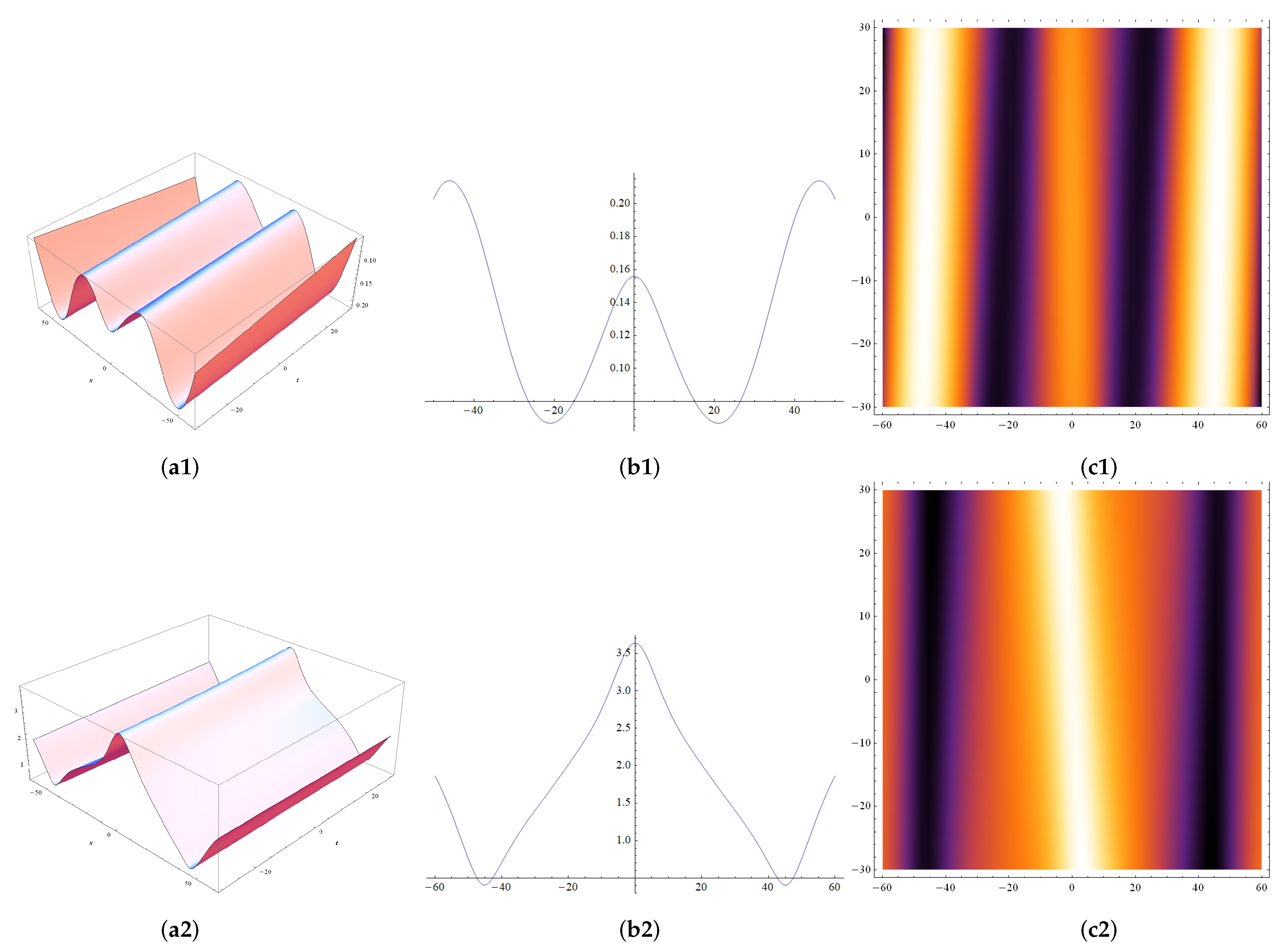
2.2. Exact Solutions for the NLS Equations

In this subsection, we will give some exact solutions of Equation (7) by applying the N-fold DT. Firstly, we give a set of seed solutions $p_1=p_2=p_3=0$ and substitute the solution into Equations (9) and (10). It is easy to find four basic solutions for these equations:

$$\psi \left(\lambda \right)=\left(\begin{array}{c}{e}^{-i\lambda x-i{\lambda }^{2}t}\\ 0\\ 0\\ 0\end{array}\right),\phi \left(\lambda \right)=\left(\begin{array}{c}0\\ e^{i\lambda x+i{\lambda }^{2}t}\\ 0\\ 0\end{array}\right),$$

(32)

$$X\left(\lambda \right)=\left(\begin{array}{c}0\\ 0\\ e^{i\lambda x+i{\lambda }^{2}t}\\ 0\end{array}\right),Y\left(\lambda \right)=\left(\begin{array}{c}0\\ 0\\ 0\\ e^{i\lambda x+i{\lambda }^{2}t}\end{array}\right).$$

(33)

Thus, substituting Equations (32) and (33) into Equation (16), we obtain

$$\left\{\begin{array}{c}{M}_j^{\left(1\right)}=\frac{v_j^{\left(1\right)}{e}^{i\lambda x+i{\lambda }^{2}t}}{e^{-i\lambda x-i{\lambda }^{2}t}}=v_j^{\left(1\right)}{e}^{2(i{\lambda }_{j}x+i{\lambda }_j^{2}t)},\hfill \\ M_j^{\left(2\right)}=\frac{v_j^{\left(2\right)}{e}^{i\lambda x+i{\lambda }^{2}t}}{e^{-i\lambda x-i{\lambda }^{2}t}}=v_j^{\left(2\right)}{e}^{2(i{\lambda }_{j}x+i{\lambda }_j^{2}t)},\hfill \\ M_j^{\left(3\right)}=\frac{v_j^{\left(3\right)}{e}^{i\lambda x+i{\lambda }^{2}t}}{e^{-i\lambda x-i{\lambda }^{2}t}}=v_j^{\left(3\right)}{e}^{2(i{\lambda }_{j}x+i{\lambda }_j^{2}t)}.\hfill \end{array}\right.$$

(34)

By using Equations (11) and (17), we have the matrix T as following

$$T=\left(\begin{array}{cccc}{\lambda }^N+\sum _{i=0}^{N-1}{A}_{11}^{\left(i\right)}{\lambda }^i& \sum _{i=0}^{N-1}{A}_{12}^{\left(i\right)}{\lambda }^i& \sum _{i=0}^{N-1}{A}_{13}^{\left(i\right)}{\lambda }^i& \sum _{i=0}^{N-1}{A}_{14}^{\left(i\right)}{\lambda }^i\\ \sum _{i=0}^{N-1}{A}_{21}^{\left(i\right)}{\lambda }^i& {\lambda }^N+\sum _{i=0}^{N-1}{A}_{22}^{\left(i\right)}{\lambda }^i;& \sum _{i=0}^{N-1}{A}_{23}^{\left(i\right)}{\lambda }^i& \sum _{i=0}^{N-1}{A}_{24}^{\left(i\right)}{\lambda }^i\\ \sum _{i=0}^{N-1}{A}_{31}^{\left(i\right)}{\lambda }^i& \sum _{i=0}^{N-1}{A}_{32}^{\left(i\right)}{\lambda }^i& {\lambda }^N+\sum _{i=0}^{N-1}{A}_{33}^{\left(i\right)}{\lambda }^i& \sum _{i=0}^{N-1}{A}_{34}^{\left(i\right)}{\lambda }^i\\ \sum _{i=0}^{N-1}{A}_{41}^{\left(i\right)}{\lambda }^i& \sum _{i=0}^{N-1}{A}_{42}^{\left(i\right)}{\lambda }^i& \sum _{i=0}^{N-1}{A}_{43}^{\left(i\right)}{\lambda }^i& {\lambda }^N+\sum _{i=0}^{N-1}{A}_{44}^{\left(i\right)}{\lambda }^i\end{array}\right),$$

(35)

and

$$\left\{\begin{array}{c}\sum _{i=0}^{N-1}(A_{11}^{\left(i\right)}+A_{12}^{\left(i\right)}{M}_j^{\left(1\right)}+A_{13}^{\left(i\right)}{M}_j^{\left(2\right)}+A_{14}^{\left(i\right)}{M}_j^{\left(3\right)}){\lambda }_j^i+{\lambda }_j^N=0,\hfill \\ \sum _{i=0}^{N-1}(A_{21}^{\left(i\right)}+A_{22}^{\left(i\right)}{M}_j^{\left(1\right)}+A_{23}^{\left(i\right)}{M}_j^{\left(2\right)}+A_{24}^{\left(i\right)}{M}_j^{\left(3\right)}){\lambda }_j^i+M_j^{\left(1\right)}{\lambda }_j^N=0,\hfill \\ \sum _{i=0}^{N-1}(A_{31}^{\left(i\right)}+A_{32}^{\left(i\right)}{M}_j^{\left(1\right)}+A_{33}^{\left(i\right)}{M}_j^{\left(2\right)}+A_{34}^{\left(i\right)}{M}_j^{\left(3\right)}){\lambda }_j^i+M_j^{\left(2\right)}{\lambda }_j^N=0,\hfill \\ \sum _{i=0}^{N-1}(A_{41}^{\left(i\right)}+A_{42}^{\left(i\right)}{M}_j^{\left(1\right)}+A_{43}^{\left(i\right)}{M}_j^{\left(2\right)}+A_{44}^{\left(i\right)}{M}_j^{\left(3\right)}){\lambda }_j^i+M_j^{\left(3\right)}{\lambda }_j^N=0.\hfill \end{array}\right.$$

(36)

Solving Equation (15) via the Gramer’s rule [21], we have

$$A_{12}^{\left(N\right)}=\frac{\Delta A_{12}^{\left(N\right)}}{{\Delta }^{\left(N\right)}},A_{13}^{\left(N\right)}=\frac{\Delta A_{13}^{\left(N\right)}}{{\Delta }^{\left(N\right)}},A_{14}^{\left(N\right)}=\frac{\Delta A_{14}^{\left(N\right)}}{{\Delta }^{\left(N\right)}},$$

(37)

with

$${\Delta }^{\left(N\right)}=\left|\begin{array}{ccccccccc}{\lambda }_1^0& \cdots & {\lambda }_1^{N-1}& M_1^{\left(1\right)}{\lambda }_1^0& \cdots & M_1^{\left(1\right)}{\lambda }_1^{N-1}& M_1^{\left(2\right)}{\lambda }_1^0& \cdots & M_1^{\left(3\right)}{\lambda }_1^{N-1}\\ {\lambda }_2^0& \cdots & {\lambda }_2^{N-1}& M_2^{\left(1\right)}{\lambda }_2^0& \cdots & M_2^{\left(1\right)}{\lambda }_2^{N-1}& M_2^{\left(2\right)}{\lambda }_2^0& \cdots & M_2^{\left(3\right)}{\lambda }_2^{N-1}\\ {\lambda }_3^0& \cdots & {\lambda }_3^{N-1}& M_3^{\left(1\right)}{\lambda }_3^0& \cdots & M_3^{\left(1\right)}{\lambda }_3^{N-1}& M_3^{\left(2\right)}{\lambda }_3^0& \cdots & M_3^{\left(3\right)}{\lambda }_3^{N-1}\\ \cdots & \cdots & \cdots & \cdots & \cdots & \cdots & \cdots & \ddots & \cdots \\ {\lambda }_{4N}^0& \cdots & {\lambda }_{4N}^{N-1}& M_{4N}^{\left(1\right)}{\lambda }_{4N}^0& \cdots & M_{4N}^{\left(1\right)}{\lambda }_{4N}^{N-1}& M_{4N}^{\left(2\right)}{\lambda }_{4N}^0& \cdots & M_{4N}^{\left(3\right)}{\lambda }_{4N}^{N-1}\end{array}\right|,$$

(38)

$$\Delta A_{12}^{\left(N\right)}=\left|\begin{array}{ccccccccc}{\lambda }_1^0& \cdots & {\lambda }_1^{N-1}& M_1^{\left(1\right)}{\lambda }_1^0& \cdots & -{\lambda }_1^N& M_1^{\left(2\right)}{\lambda }_1^0& \cdots & M_1^{\left(3\right)}{\lambda }_1^{N-1}\\ {\lambda }_2^0& \cdots & {\lambda }_2^{N-1}& M_2^{\left(1\right)}{\lambda }_2^0& \cdots & -{\lambda }_2^N& M_2^{\left(2\right)}{\lambda }_2^0& \cdots & M_2^{\left(3\right)}{\lambda }_2^{N-1}\\ {\lambda }_3^0& \cdots & {\lambda }_3^{N-1}& M_3^{\left(1\right)}{\lambda }_3^0& \cdots & -{\lambda }_3^N& M_3^{\left(2\right)}{\lambda }_3^0& \cdots & M_3^{\left(3\right)}{\lambda }_3^{N-1}\\ \cdots & \cdots & \cdots & \cdots & \cdots & \cdots & \cdots & \ddots & \cdots \\ {\lambda }_{4N}^0& \cdots & {\lambda }_{4N}^{N-1}& M_{4N}^{\left(1\right)}{\lambda }_{4N}^0& \cdots & -{\lambda }_{4N}^N& M_{4N}^{\left(2\right)}{\lambda }_{4N}^0& \cdots & M_{4N}^{\left(3\right)}{\lambda }_{4N}^{N-1}\end{array}\right|,$$

(39)

$$\Delta A_{13}^{\left(N\right)}=\left|\begin{array}{ccccccccc}{\lambda }_1^0& \cdots & {\lambda }_1^{N-1}& M_1^{\left(1\right)}{\lambda }_1^0& \cdots & M_1^{\left(2\right)}{\lambda }_1^0& -{\lambda }_1^N& \cdots & M_1^{\left(3\right)}{\lambda }_1^{N-1}\\ {\lambda }_2^0& \cdots & {\lambda }_2^{N-1}& M_2^{\left(1\right)}{\lambda }_2^0& \cdots & M_2^{\left(2\right)}{\lambda }_2^0& -{\lambda }_2^N& \cdots & M_2^{\left(3\right)}{\lambda }_2^{N-1}\\ {\lambda }_3^0& \cdots & {\lambda }_3^{N-1}& M_3^{\left(1\right)}{\lambda }_3^0& \cdots & M_3^{\left(2\right)}{\lambda }_3^0& -{\lambda }_3^N& \cdots & M_3^{\left(3\right)}{\lambda }_3^{N-1}\\ \cdots & \cdots & \cdots & \cdots & \cdots & \cdots & \cdots & \ddots & \cdots \\ {\lambda }_{4N}^0& \cdots & {\lambda }_{4N}^{N-1}& M_{4N}^{\left(1\right)}{\lambda }_{4N}^0& \cdots & M_{4N}^{\left(2\right)}{\lambda }_{4N}^0& -{\lambda }_{4N}^N& \cdots & M_{4N}^{\left(3\right)}{\lambda }_{4N}^{N-1}\end{array}\right|,$$

(40)

$$\Delta A_{14}^{\left(N\right)}=\left|\begin{array}{ccccccccc}{\lambda }_1^0& \cdots & {\lambda }_1^{N-1}& M_1^{\left(1\right)}{\lambda }_1^0& \cdots & M_1^{\left(1\right)}{\lambda }_1^{N-1}& M_1^{\left(2\right)}{\lambda }_1^0& \cdots & -{\lambda }_1^N\\ {\lambda }_2^0& \cdots & {\lambda }_2^{N-1}& M_2^{\left(1\right)}{\lambda }_2^0& \cdots & M_2^{\left(1\right)}{\lambda }_2^{N-1}& M_2^{\left(2\right)}{\lambda }_2^0& \cdots & -{\lambda }_2^N\\ {\lambda }_3^0& \cdots & {\lambda }_3^{N-1}& M_3^{\left(1\right)}{\lambda }_3^0& \cdots & M_3^{\left(1\right)}{\lambda }_3^{N-1}& M_3^{\left(2\right)}{\lambda }_3^0& \cdots & -{\lambda }_3^N\\ \cdots & \cdots & \cdots & \cdots & \cdots & \cdots & \cdots & \ddots & \cdots \\ {\lambda }_{4N}^0& \cdots & {\lambda }_{4N}^{N-1}& M_{4N}^{\left(1\right)}{\lambda }_{4N}^0& \cdots & M_{4N}^{\left(1\right)}{\lambda }_{4N}^{N-1}& M_{4N}^{\left(2\right)}{\lambda }_{4N}^0& \cdots & -{\lambda }_{4N}^N\end{array}\right|.$$

(41)

with $M_j^{\left(1\right)}=v_j^{\left(1\right)}{e}^{2i({\lambda }_{j}x+{\lambda }_j^{2}t)}$, $M_j^{\left(2\right)}=v_j^{\left(2\right)}{e}^{2i({\lambda }_{j}x+{\lambda }_j^{2}t)}$, $M_j^{\left(3\right)}=v_j^{\left(3\right)}{e}^{2i({\lambda }_{j}x+{\lambda }_j^{2}t)}$$(1\le j\le 4N)$.

Using Equations (11), (12), (20) and (37), we can derive the solutions for the NLS Equation (7)

$$\left\{\begin{array}{c}\widetilde{p_1}=2A_{12}^{\left(N\right)}=2\frac{\Delta A_{12}^{\left(N\right)}}{{\Delta }^{\left(N\right)}},\hfill \\ \widetilde{p_2}=2A_{13}^{\left(N\right)}=2\frac{\Delta A_{13}^{\left(N\right)}}{{\Delta }^{\left(N\right)}},\hfill \\ \widetilde{p_3}=2A_{14}^{\left(N\right)}=2\frac{\Delta A_{14}^{\left(N\right)}}{{\Delta }^{\left(N\right)}}.\hfill \end{array}\right.$$

(42)

Now, we consider $N=1,2$ respectively, and draw these plane graphs and the density plots as Figure 1 and Figure 2.

(1) Firstly, we consider $N=1$, $\lambda ={\lambda }_j(j=1,2,3,4)$ in Equations (12) and (17), and obtain the matrix T

$$T=\left(\begin{array}{cccc}\lambda +A_{11}& A_{12}& A_{13}& A_{14}\\ A_{21}& \lambda +A_{22}& A_{23}& A_{24}\\ A_{31}& A_{32}& \lambda +A_{33}& A_{34}\\ A_{41}& A_{42}& A_{43}& \lambda +A_{44}\end{array}\right),$$

(43)

and

$$\left\{\begin{array}{c}{\lambda }_j+A_{11}+M_j^{\left(1\right)}{A}_{12}+M_j^{\left(2\right)}{A}_{13}+M_j^{\left(3\right)}{A}_{14}=0,\hfill \\ A_{21}+M_j^{\left(1\right)}(A_{22}+{\lambda }_j)+M_j^{\left(2\right)}{A}_{23}+M_j^{\left(3\right)}{A}_{24}=0,\hfill \\ A_{31}+M_j^{\left(2\right)}(A_{33}+{\lambda }_j)+M_j^{\left(1\right)}{A}_{32}+M_j^{\left(3\right)}{A}_{34}=0,\hfill \\ A_{41}+M_j^{\left(3\right)}(A_{44}+{\lambda }_j)+M_j^{\left(1\right)}{A}_{42}+M_j^{\left(2\right)}{A}_{43}=0.\hfill \end{array}\right.$$

(44)

According to Equations (38)–(41), we get

$${\Delta }^{\left(1\right)}=\left|\begin{array}{cccc}1& M_1^{\left(1\right)}& M_1^{\left(2\right)}& M_1^{\left(3\right)}\\ 1& M_2^{\left(1\right)}& M_2^{\left(2\right)}& M_2^{\left(3\right)}\\ 1& M_3^{\left(1\right)}& M_3^{\left(2\right)}& M_3^{\left(3\right)}\\ 1& M_4^{\left(1\right)}& M_4^{\left(2\right)}& M_4^{\left(3\right)}\end{array}\right|,$$

(45)

$$\Delta A_{12}^{\left(1\right)}=\left|\begin{array}{cccc}1& -{\lambda }_1& M_1^{\left(2\right)}& M_1^{\left(3\right)}\\ 1& -{\lambda }_2& M_2^{\left(2\right)}& M_2^{\left(3\right)}\\ 1& -{\lambda }_3& M_3^{\left(2\right)}& M_3^{\left(3\right)}\\ 1& -{\lambda }_4& M_4^{\left(2\right)}& M_4^{\left(3\right)}\end{array}\right|,$$

(46)

$$\Delta A_{13}^{\left(1\right)}=\left|\begin{array}{cccc}1& M_1^{\left(1\right)}& -{\lambda }_1& M_1^{\left(3\right)}\\ 1& M_2^{\left(1\right)}& -{\lambda }_2& M_2^{\left(3\right)}\\ 1& M_3^{\left(1\right)}& -{\lambda }_3& M_3^{\left(3\right)}\\ 1& M_4^{\left(1\right)}& -{\lambda }_4& M_4^{\left(3\right)}\end{array}\right|,$$

(47)

$$\Delta A_{14}^{\left(1\right)}=\left|\begin{array}{cccc}1& M_1^{\left(1\right)}& M_1^{\left(2\right)}& -{\lambda }_1\\ 1& M_2^{\left(1\right)}& M_2^{\left(2\right)}& -{\lambda }_2\\ 1& M_3^{\left(1\right)}& M_3^{\left(2\right)}& -{\lambda }_3\\ 1& M_4^{\left(1\right)}& M_4^{\left(2\right)}& -{\lambda }_4\end{array}\right|.$$

(48)

Based on Equation (37), we obtain the following systems

$$A_{12}^{\left(1\right)}=\frac{\Delta A_{12}^{\left(1\right)}}{{\Delta }^{\left(1\right)}},A_{13}^{\left(1\right)}=\frac{\Delta A_{13}^{\left(1\right)}}{{\Delta }^{\left(1\right)}},A_{14}^{\left(1\right)}=\frac{\Delta A_{14}^{\left(1\right)}}{{\Delta }^{\left(1\right)}}.$$

(49)

Thus, the exact solutions of Equation (7) are obtained by the DT method as follows

$$\left\{\begin{array}{c}\widetilde{p_1}=2A_{12}^{\left(1\right)}=2\frac{\Delta A_{12}^{\left(1\right)}}{{\Delta }^{\left(1\right)}},\hfill \\ \widetilde{p_2}=2A_{13}^{\left(1\right)}=2\frac{\Delta A_{13}^{\left(1\right)}}{{\Delta }^{\left(1\right)}},\hfill \\ \widetilde{p_3}=2A_{14}^{\left(1\right)}=2\frac{\Delta A_{14}^{\left(1\right)}}{{\Delta }^{\left(1\right)}}.\hfill \end{array}\right.$$

(50)

To illustrate the exact solution (58), we can select some free parameters in the form ${\lambda }_1$, ${\lambda }_2$, ${\lambda }_3$, ${\lambda }_4$, $v_m^{\left(k\right)}$$(m=1,2,3,4,k=1,2,3)$. Figure 1 shows the exact solutions to Equation (50).

(2) Nextly, we consider $N=2$, $\lambda ={\lambda }_j(j=1,2,3,4,5,6,7,8)$ in Equations (12) and (17), and obtain the matrix T

$$T=\left(\begin{array}{cccc}{\lambda }^2+A_{11}^{\left(1\right)}\lambda +A_{11}^{\left(0\right)}& A_{12}^{\left(1\right)}\lambda +A_{12}^{\left(0\right)}& A_{13}^{\left(1\right)}\lambda +A_{13}^{\left(0\right)}& A_{14}^{\left(1\right)}\lambda +A_{14}^{\left(0\right)}\\ A_{21}^{\left(1\right)}\lambda +A_{21}^{\left(0\right)}& {\lambda }^2+A_{22}^{\left(1\right)}\lambda +A_{22}^{\left(0\right)}& A_{23}^{\left(1\right)}\lambda +A_{23}^{\left(0\right)}& A_{24}^{\left(1\right)}\lambda +A_{24}^{\left(0\right)}\\ A_{31}^{\left(1\right)}\lambda +A_{31}^{\left(0\right)}& A_{32}^{\left(1\right)}\lambda +A_{32}^{\left(0\right)}& {\lambda }^2+A_{33}^{\left(1\right)}\lambda +A_{33}^{\left(0\right)}& A_{34}^{\left(1\right)}\lambda +A_{34}^{\left(0\right)}\\ A_{41}^{\left(1\right)}\lambda +A_{41}^{\left(0\right)}& A_{42}^{\left(1\right)}\lambda +A_{42}^{\left(0\right)}& A_{43}^{\left(1\right)}\lambda +A_{43}^{\left(0\right)}& {\lambda }^2+A_{44}^{\left(1\right)}\lambda +A_{44}^{\left(0\right)}\end{array}\right),$$

(51)

$$\left\{\begin{array}{c}{M}_j^{\left(1\right)}[A_{12}^{\left(0\right)}+A_{12}^{\left(1\right)}{\lambda }_j]+M_j^{\left(2\right)}[A_{13}^{\left(0\right)}+A_{13}^{\left(1\right)}{\lambda }_j]+M_j^{\left(3\right)}[A_{14}^{\left(0\right)}+A_{14}^{\left(1\right)}{\lambda }_j]+[A_{11}^{\left(0\right)}+A_{11}^{\left(1\right)}{\lambda }_j+{\lambda }_j^2]=0,\hfill \\ M_j^{\left(1\right)}[{\lambda }_j^2+A_{22}^{\left(1\right)}{\lambda }_j+A_{22}^{\left(0\right)}]+M_j^{\left(2\right)}[A_{23}^{\left(1\right)}{\lambda }_j+A_{23}^{\left(0\right)}]+M_j^{\left(3\right)}[A_{24}^{\left(0\right)}+A_{24}^{\left(1\right)}{\lambda }_j]+[A_{21}^{\left(0\right)}+A_{21}^{\left(1\right)}{\lambda }_j]=0,\hfill \\ M_j^{\left(1\right)}[A_{32}^{\left(1\right)}{\lambda }_j+A_{32}^{\left(0\right)}]+M_j^{\left(2\right)}[{\lambda }_j^2+A_{33}^{\left(1\right)}{\lambda }_j+A_{33}^{\left(0\right)}]+M_j^{\left(3\right)}[A_{34}^{\left(0\right)}+A_{34}^{\left(1\right)}{\lambda }_j]+[A_{31}^{\left(0\right)}+A_{31}^{\left(1\right)}{\lambda }_j]=0,\hfill \\ M_j^{\left(1\right)}[A_{42}^{\left(1\right)}{\lambda }_j+A_{42}^{\left(0\right)}]+M_j^{\left(2\right)}[A_{43}^{\left(1\right)}{\lambda }_j+A_{43}^{\left(0\right)}]+M_j^{\left(3\right)}[{\lambda }_j^2+A_{44}^{\left(0\right)}+A_{44}^{\left(1\right)}{\lambda }_j]+[A_{41}^{\left(0\right)}+A_{41}^{\left(1\right)}{\lambda }_j]=0.\hfill \end{array}\right.$$

(52)

According to Equations (38)–(41), we get

$${\Delta }^{\left(2\right)}=\left|\begin{array}{cccccccc}1& M_1^{\left(1\right)}& M_1^{\left(2\right)}& M_1^{\left(3\right)}& {\lambda }_1& {\lambda }_1{M}_1^{\left(1\right)}& {\lambda }_1{M}_1^{\left(2\right)}& {\lambda }_1{M}_1^{\left(3\right)}\\ 1& M_2^{\left(1\right)}& M_2^{\left(2\right)}& M_2^{\left(3\right)}& {\lambda }_2& {\lambda }_2{M}_2^{\left(1\right)}& {\lambda }_2{M}_2^{\left(2\right)}& {\lambda }_2{M}_2^{\left(3\right)}\\ 1& M_3^{\left(1\right)}& M_3^{\left(2\right)}& M_3^{\left(3\right)}& {\lambda }_3& {\lambda }_3{M}_3^{\left(1\right)}& {\lambda }_3{M}_3^{\left(2\right)}& {\lambda }_3{M}_3^{\left(3\right)}\\ 1& M_4^{\left(1\right)}& M_4^{\left(2\right)}& M_4^{\left(3\right)}& {\lambda }_4& {\lambda }_4{M}_4^{\left(1\right)}& {\lambda }_4{M}_4^{\left(2\right)}& {\lambda }_4{M}_4^{\left(3\right)}\\ 1& M_5^{\left(1\right)}& M_5^{\left(2\right)}& M_5^{\left(3\right)}& {\lambda }_5& {\lambda }_5{M}_5^{\left(1\right)}& {\lambda }_5{M}_5^{\left(2\right)}& {\lambda }_5{M}_5^{\left(3\right)}\\ 1& M_6^{\left(1\right)}& M_6^{\left(2\right)}& M_6^{\left(3\right)}& {\lambda }_6& {\lambda }_6{M}_6^{\left(1\right)}& {\lambda }_6{M}_6^{\left(2\right)}& {\lambda }_6{M}_6^{\left(3\right)}\\ 1& M_7^{\left(1\right)}& M_7^{\left(2\right)}& M_7^{\left(3\right)}& {\lambda }_7& {\lambda }_7{M}_7^{\left(1\right)}& {\lambda }_7{M}_7^{\left(2\right)}& {\lambda }_7{M}_7^{\left(3\right)}\\ 1& M_8^{\left(1\right)}& M_8^{\left(2\right)}& M_8^{\left(3\right)}& {\lambda }_8& {\lambda }_8{M}_8^{\left(1\right)}& {\lambda }_8{M}_8^{\left(2\right)}& {\lambda }_8{M}_8^{\left(3\right)}\end{array}\right|,$$

(53)

$$\Delta A_{12}^{\left(2\right)}=\left|\begin{array}{cccccccc}1& M_1^{\left(1\right)}& M_1^{\left(2\right)}& M_1^{\left(3\right)}& {\lambda }_1& -{\lambda }_1^2& {\lambda }_1{M}_1^{\left(2\right)}& {\lambda }_1{M}_1^{\left(3\right)}\\ 1& M_2^{\left(1\right)}& M_2^{\left(2\right)}& M_2^{\left(3\right)}& {\lambda }_2& -{\lambda }_2^2& {\lambda }_2{M}_2^{\left(2\right)}& {\lambda }_2{M}_2^{\left(3\right)}\\ 1& M_3^{\left(1\right)}& M_3^{\left(2\right)}& M_3^{\left(3\right)}& {\lambda }_3& -{\lambda }_3^2& {\lambda }_3{M}_3^{\left(2\right)}& {\lambda }_3{M}_3^{\left(3\right)}\\ 1& M_4^{\left(1\right)}& M_4^{\left(2\right)}& M_4^{\left(3\right)}& {\lambda }_4& -{\lambda }_4^2& {\lambda }_4{M}_4^{\left(2\right)}& {\lambda }_4{M}_4^{\left(3\right)}\\ 1& M_5^{\left(1\right)}& M_5^{\left(2\right)}& M_5^{\left(3\right)}& {\lambda }_5& -{\lambda }_5^2& {\lambda }_5{M}_5^{\left(2\right)}& {\lambda }_5{M}_5^{\left(3\right)}\\ 1& M_6^{\left(1\right)}& M_6^{\left(2\right)}& M_6^{\left(3\right)}& {\lambda }_6& -{\lambda }_6^2& {\lambda }_6{M}_6^{\left(2\right)}& {\lambda }_6{M}_6^{\left(3\right)}\\ 1& M_7^{\left(1\right)}& M_7^{\left(2\right)}& M_7^{\left(3\right)}& {\lambda }_7& -{\lambda }_7^2& {\lambda }_7{M}_7^{\left(2\right)}& {\lambda }_7{M}_7^{\left(3\right)}\\ 1& M_8^{\left(1\right)}& M_8^{\left(2\right)}& M_8^{\left(3\right)}& {\lambda }_8& -{\lambda }_8^2& {\lambda }_8{M}_8^{\left(2\right)}& {\lambda }_8{M}_8^{\left(3\right)}\end{array}\right|,$$

(54)

$$\Delta A_{13}^{\left(2\right)}=\left|\begin{array}{cccccccc}1& M_1^{\left(1\right)}& M_1^{\left(2\right)}& M_1^{\left(3\right)}& {\lambda }_1& {\lambda }_1{M}_1^{\left(1\right)}& -{\lambda }_1^2& {\lambda }_1{M}_1^{\left(3\right)}\\ 1& M_2^{\left(1\right)}& M_2^{\left(2\right)}& M_2^{\left(3\right)}& {\lambda }_2& {\lambda }_2{M}_2^{\left(1\right)}& -{\lambda }_2^2& {\lambda }_2{M}_2^{\left(3\right)}\\ 1& M_3^{\left(1\right)}& M_3^{\left(2\right)}& M_3^{\left(3\right)}& {\lambda }_3& {\lambda }_3{M}_3^{\left(1\right)}& -{\lambda }_3^2& {\lambda }_3{M}_3^{\left(3\right)}\\ 1& M_4^{\left(1\right)}& M_4^{\left(2\right)}& M_4^{\left(3\right)}& {\lambda }_4& {\lambda }_4{M}_4^{\left(1\right)}& -{\lambda }_4^2& {\lambda }_4{M}_4^{\left(3\right)}\\ 1& M_5^{\left(1\right)}& M_5^{\left(2\right)}& M_5^{\left(3\right)}& {\lambda }_5& {\lambda }_5{M}_5^{\left(1\right)}& -{\lambda }_5^2& {\lambda }_5{M}_5^{\left(3\right)}\\ 1& M_6^{\left(1\right)}& M_6^{\left(2\right)}& M_6^{\left(3\right)}& {\lambda }_6& {\lambda }_6{M}_6^{\left(1\right)}& -{\lambda }_6^2& {\lambda }_6{M}_6^{\left(3\right)}\\ 1& M_7^{\left(1\right)}& M_7^{\left(2\right)}& M_7^{\left(3\right)}& {\lambda }_7& {\lambda }_7{M}_7^{\left(1\right)}& -{\lambda }_7^2& {\lambda }_7{M}_7^{\left(3\right)}\\ 1& M_8^{\left(1\right)}& M_8^{\left(2\right)}& M_8^{\left(3\right)}& {\lambda }_8& {\lambda }_8{M}_8^{\left(1\right)}& -{\lambda }_8^2& {\lambda }_8{M}_8^{\left(3\right)}\end{array}\right|,$$

(55)

$$\Delta A_{14}^{\left(2\right)}=\left|\begin{array}{cccccccc}1& M_1^{\left(1\right)}& M_1^{\left(2\right)}& M_1^{\left(3\right)}& {\lambda }_1& {\lambda }_1{M}_1^{\left(1\right)}& {\lambda }_1{M}_1^{\left(2\right)}& -{\lambda }_1^2\\ 1& M_2^{\left(1\right)}& M_2^{\left(2\right)}& M_2^{\left(3\right)}& {\lambda }_2& {\lambda }_2{M}_2^{\left(1\right)}& {\lambda }_2{M}_2^{\left(2\right)}& -{\lambda }_2^2\\ 1& M_3^{\left(1\right)}& M_3^{\left(2\right)}& M_3^{\left(3\right)}& {\lambda }_3& {\lambda }_3{M}_3^{\left(1\right)}& {\lambda }_3{M}_3^{\left(2\right)}& -{\lambda }_3^2\\ 1& M_4^{\left(1\right)}& M_4^{\left(2\right)}& M_4^{\left(3\right)}& {\lambda }_4& {\lambda }_4{M}_4^{\left(1\right)}& {\lambda }_4{M}_4^{\left(2\right)}& -{\lambda }_4^2\\ 1& M_5^{\left(1\right)}& M_5^{\left(2\right)}& M_5^{\left(3\right)}& {\lambda }_5& {\lambda }_5{M}_5^{\left(1\right)}& {\lambda }_5{M}_5^{\left(2\right)}& -{\lambda }_5^2\\ 1& M_6^{\left(1\right)}& M_6^{\left(2\right)}& M_6^{\left(3\right)}& {\lambda }_6& {\lambda }_6{M}_6^{\left(1\right)}& {\lambda }_6{M}_6^{\left(2\right)}& -{\lambda }_6^2\\ 1& M_7^{\left(1\right)}& M_7^{\left(2\right)}& M_7^{\left(3\right)}& {\lambda }_7& {\lambda }_7{M}_7^{\left(1\right)}& {\lambda }_7{M}_7^{\left(2\right)}& -{\lambda }_7^2\\ 1& M_8^{\left(1\right)}& M_8^{\left(2\right)}& M_8^{\left(3\right)}& {\lambda }_8& {\lambda }_8{M}_8^{\left(1\right)}& {\lambda }_8{M}_8^{\left(2\right)}& -{\lambda }_8^2\end{array}\right|.$$

(56)

Based on Equation (37), we obtain the following systems

$$A_{12}^{\left(2\right)}=\frac{\Delta A_{12}^{\left(2\right)}}{{\Delta }^{\left(2\right)}},A_{13}^{\left(2\right)}=\frac{\Delta A_{13}^{\left(2\right)}}{{\Delta }^{\left(2\right)}},A_{14}^{\left(2\right)}=\frac{\Delta A_{14}^{\left(2\right)}}{{\Delta }^{\left(2\right)}}.$$

(57)

The analytic soliton solutions of the equations are obtained by the DT method as follows

$$\left\{\begin{array}{c}\widetilde{p_1}=2A_{12}^{\left(2\right)}=2\frac{\Delta A_{12}^{\left(2\right)}}{{\Delta }^{\left(2\right)}},\hfill \\ \widetilde{p_2}=2A_{13}^{\left(2\right)}=2\frac{\Delta A_{13}^{\left(2\right)}}{{\Delta }^{\left(2\right)}},\hfill \\ \widetilde{p_3}=2A_{14}^{\left(2\right)}=2\frac{\Delta A_{14}^{\left(2\right)}}{{\Delta }^{\left(2\right)}}.\hfill \end{array}\right.$$

(58)

To illustrate the exact solution (58), we can select some free parameters in the form ${\lambda }_1$, ${\lambda }_2$, ${\lambda }_3$, ${\lambda }_4$, ${\lambda }_5$, ${\lambda }_6$, ${\lambda }_7$, ${\lambda }_8$, $v_m^{\left(k\right)}$ (m = 1, 2, 3, 4, 5, 6, 7, 8, k = 1, 2, 3). Figure 2 shows the exact solutions to Equation (58).

3. Conclusions

In this paper, we constructed DT for the NLS Equation (7). Through using the Gramers rule [21] and selecting the appropriate parameters, we give the expressions of N-exact solutions, and 1- and 2-fold exact solutions. By solving the three-component NLS equations, we find that it is quite different from the solution of the NLS equation. In the future work, we want to consider the initial solution besides zero, and try to obtain the DT of the coupled nonlocal equation.

References

1. Matveev, V.B.; Salle, M.A. Darboux Transformations and Solitons; Springer: Berlin/Heidelberg, Germany, 1991. [Google Scholar]
2. Gu, C.-H.; Hu, H.-S.; Zhou, Z.-X. Darboux Transformation of Soliton Theory and Its Geometric Application; Shanghai Science and Technology Press: Shanghai, China, 1999. [Google Scholar]
3. Ablowitz, M.J.; Ablowitz, M.A.; Clarkson, P.A. Solitons Nonlinear Evolution Equations and In-Verse Scattering; Cambridge University Press: Cambridge, UK, 1991. [Google Scholar]
4. Ma, W.-X. Darboux transformations for a Lax integrable system in 2n-dimensions. Lett. Math. Phys. 1997, 39, 33–49. [Google Scholar] [CrossRef] [Green Version]
5. Ma, W.-X.; Zhang, J.Y. Darboux transformatins of integrable couplings and applications. Rev. Math. Phys. 2018, 30, 1850003. [Google Scholar] [CrossRef]
6. Geng, X.-G. Darboux transformation of the discrete Ablowitz–Ladik eigenvalue problem. Acta Math. Sci. 1989, 9, 21–26. [Google Scholar] [CrossRef]
7. Bagrov, V.G.; Samsonov, B.F. Darboux transformation of the Schrödinger equation. Phys. Part. Nuclei 1997, 28, 374–397. [Google Scholar] [CrossRef]
8. Xin, X.-P.; Xia, Y.-R.; Liu, H.-Z.; Zhang, L.L. Darboux transformation of the variable coefficient nonlocal equation. J. Math. Anal. Appl. 2020, 490, 124–227. [Google Scholar] [CrossRef]
9. Gürsesl, M.; Pekcan, A. Nonlocal nonlinear Schrödinger equations and their soliton solutions. J. Math. Phys. 2018, 59, 051501. [Google Scholar] [CrossRef] [Green Version]
10. Yang, B.; Chen, Y. Several reverse-time integrable nonlocal nonlinear equations: Rogue-wave solutions. Chaos 2018, 28, 053104. [Google Scholar] [CrossRef] [PubMed]
11. Meng, D.-X.; Li, K.-Z. Darboux transformation of the second-type nonlocal derivative nonlinear Schrödinger equation. Mod. Phys. Lett. B 2019, 33, 1950123. [Google Scholar] [CrossRef]
12. Ablowitz, M.J.; Prinari, B.; Trubatch, A.D. Discrete and Continuous Nonlinear Schrödinger Systems; Cambridge University Press: Cambridge, UK, 2004. [Google Scholar]
13. Duval, C.; Horvthy, P.A. On Schrödinger superalgebras. J. Math. Phys. 1994, 35, 2516. [Google Scholar] [CrossRef] [Green Version]
14. Leblanc, M.; Lozano, G.; Min, H. Extended superconformal Galilean symmetry in Chern–Simons matter systems. Ann. Phys. 1992, 219, 328–348. [Google Scholar] [CrossRef] [Green Version]
15. Nakayama, Y.; Sakaguchi, M.; Yoshida, K. Non-relativistic M2-brane gauge theory and new superconformal algebra. J. High. Energy Phys. 2009, 941–944. [Google Scholar] [CrossRef] [Green Version]
16. Galajinsky, A.; Masterov, I. Remark on quantum mechanics with N = 2 Schrödinger supersymmetry. Phys. Lett. B. 2009, 675, 116. [Google Scholar] [CrossRef]
17. Malomed, B.A.; Mihalache, D.; Wise, F.; Torner, L. Spatiotemporal optical solitons. J. Opt. B Quantum Semiclass. Opt. 2005, 7, R53–R72. [Google Scholar] [CrossRef]
18. Carretero-Gonzalez, R.; Frantzeskakis, D.J.; Kevrekidis, P.G. Nonlinear waves in Bose–Einstein condensates. Nonlinearity 2008, 21, R139–R202. [Google Scholar] [CrossRef] [Green Version]
19. Yan, Z.-Y. Nonlocal general vector nonlinear Schrödinger equations: Integrability, PT symmetribility, and solutions. Appl. Math. Lett. 2016, 62, 101–109. [Google Scholar] [CrossRef]
20. Yan, Z.Y.; Konotop, V.V. Exact solutions to threedimensional generalized nonlinear Schrödinger equa-tions with varying potential and nonlinearities. Phys. Rev. E 2009, 80, 036607. [Google Scholar] [CrossRef] [PubMed] [Green Version]
21. Yu, F.J. Nonautonomous rogue waves and ‘catch’ dynamics for the combined Hirota-LPD equation with variable coefficients. Commun. Nonlinear. Sci. Numer. Simul. 2016, 34, 142–153. [Google Scholar] [CrossRef]
22. Malomed, B.; Torner, L.; Wise, F.; Mihalache, D. On multidimensional solitons and their legacy in contem-poraryatomic, molecular and optical physics. J. Phys. B Mol. Opt. Phys. 2016, 49, 170502. [Google Scholar] [CrossRef] [Green Version]
23. Yu, F.; Feng, L.; Li, L. Darboux transformations for super-Schrödinger equation, super-Dirac equation and their exact solutions. Nonlinear Dyn. 2017, 88, 1257–1271. [Google Scholar] [CrossRef]
24. Ablowitz, M.J.; Musslimani, Z.H. Integrable nonlocal nonlinear Schrödinger equation. Phys. Rev. Lett. 2013, 110, 064105. [Google Scholar] [CrossRef] [Green Version]
25. Ablowitz, M.J.; Musslimani, Z.H. Integrable nonlocal nonlinear equations. Stud. Appl. Math. 2017, 139, 7–59. [Google Scholar] [CrossRef] [Green Version]
26. Yan, Z.Y.; Hang, C. Analytical three-dimensional bright solitons and soliton-pairs in Bose–Einstein conden-sates with time-space modulation. Phys. Rev. A 2009, 80, 063626. [Google Scholar] [CrossRef] [Green Version]
27. Hovhannisyan, G.; Ruff, O. Darboux transformations on a space scale. J. Math. Anal. Appl. 2016, 434, 1690–1718. [Google Scholar] [CrossRef]
28. Duan, C.; Yu, F. N-Fold Darboux Transformation for the Nonlocal Nonlinear Schrödinger (NNLS) Equation with the Self-Induced PT-Symmetric Potential. J. Appl. Math. Phys. 2018, 6, 888–900. [Google Scholar] [CrossRef] [Green Version]
29. Hobby, D.; Shemyakova, E. Classification of Multidimensional Darboux Transformations: First Order and Continued Type. Symmetry Integr. Geom. Methods Appl. 2017, 13, 010. [Google Scholar] [CrossRef] [Green Version]
30. Ma, W.X.; Batwa, S. A binary Darboux transformation for multicomponent NLS equations and their reduc-tions. Anal. Math. Phys. 2021, 11, 44. [Google Scholar] [CrossRef]
31. Ablowitz, M.J.; Kaup, D.J.; Newell, A.C.; Segur, H. The inverse scattering transform-Fourier analysis for nonlinear problems. Stud. Appl. Math. 1974, 53, 249–315. [Google Scholar] [CrossRef]
32. Ma, W.X. Integrable couplings of vector AKNS soliton equations. J. Math. Phys. 2005, 46, 033507. [Google Scholar] [CrossRef]
33. Ma, W.X.; Wu, H. Time–space integrable decompositions of nonlinear evolution equations. J. Math. Anal. Appl. 2006, 324, 134–149. [Google Scholar] [CrossRef] [Green Version]
34. Ma, W.X. Multi-component bi-Hamiltonian Dirac integrable equations. Chaos Solitons Fractals 2009, 39, 282–287. [Google Scholar] [CrossRef]
35. Ma, W.X. Long-time asymptotics of a three-component coupled nonlinear Schrödinger system. J. Geom. Phys. 2020, 153, 103669. [Google Scholar] [CrossRef]
36. Yu, J.; Chen, S.-T.; Ma, W.X. N-fold Darboux Transformation for Integrable Couplings of AKNS Equations. Commun. Theor. Phys. 2018, 69, 367. [Google Scholar] [CrossRef] [Green Version]
Figure 1. (a1a3) are the first-fold exact solutions p ˜ 1 , p ˜ 2 , p ˜ 3 of Equation (48); (b1b3) are the plane graphs of p ˜ 1 , p ˜ 2 , p ˜ 3 of Equation (48) at t = 0 ; (c1c3) are the density plots of p ˜ 1 , p ˜ 2 , p ˜ 3 of Equation (48) with λ 1 = 0.1 , λ 2 = 0.4 , λ 3 = 0.3 , λ 4 = 0.2 , v 1 ( 1 ) = 0.01 , v 2 ( 1 ) = 0.3 , v 3 ( 1 ) = 0.4 , v 4 ( 1 ) = 0.05 , v 1 ( 2 ) = 0.1 , v 2 ( 2 ) = 0.02 , v 3 ( 2 ) = 0.04 , v 4 ( 2 ) = 0.6 , v 1 ( 3 ) = 0.03 , v 2 ( 3 ) = 0.2 , v 3 ( 3 ) = 0.5 , v 4 ( 3 ) = 0.06 .
Mathematics 09 00733 g001
Figure 2. (a1a3) are the second-fold exact solutions p ˜ 1 , p ˜ 2 , p ˜ 3 of Equation (56); (b1b3) are plane graphs p ˜ 1 , p ˜ 2 , p ˜ 3 of Equation (56) at t = 0 ; (c1c3) are the density plots of p ˜ 1 , p ˜ 2 , p ˜ 3 of Equation (56) with λ 1 = 0.01 , λ 2 = 0.04 , λ 3 = 0.03 , λ 4 = 0.02 , λ 5 = 0.05 , λ 6 = 0.06 , λ 7 = 0.07 , λ 8 = 0.08 , v 1 ( 1 ) = 0.1 , v 2 ( 1 ) = 0.3 , v 3 ( 1 ) = 0.6 , v 4 ( 1 ) = 0.9 , v 5 ( 1 ) = 0.3 , v 6 ( 1 ) = 0.6 , v 7 ( 1 ) = 0.9 , v 8 ( 1 ) = 0.14 , v 1 ( 2 ) = 0.1 , v 2 ( 2 ) = 0.4 , v 3 ( 2 ) = 0.7 , v 4 ( 2 ) = 0.2 , v 5 ( 2 ) = 0.4 , v 6 ( 2 ) = 0.7 , v 7 ( 2 ) = 0.12 , v 8 ( 2 ) = 0.15 , v 1 ( 3 ) = 0.2 , v 2 ( 3 ) = 0.5 , v 3 ( 3 ) = 0.8 , v 4 ( 3 ) = 0.11 , v 5 ( 3 ) = 0.5 , v 6 ( 3 ) = 0.8 , v 7 ( 3 ) = 0.13 , v 8 ( 3 ) = 0.16 .
Mathematics 09 00733 g002aMathematics 09 00733 g002b
Publisher’s Note: MDPI stays neutral with regard to jurisdictional claims in published maps and institutional affiliations.