Article

Method of Constructing a Nonlinear Approximating Scheme of a Complex Signal: Application Pattern Recognition

by
Oksana Mandrikova
,
Bogdana Mandrikova
* and
Anastasia Rodomanskay
Institute of Cosmophysical Research and Radio Wave Propagation, Far Eastern Branch of the Russian Academy of Sciences, Mirnaya st, 7, Paratunka, 684034 Kamchatskiy Kray, Russia
*
Author to whom correspondence should be addressed.
Mathematics 2021, 9(7), 737; https://doi.org/10.3390/math9070737
Submission received: 31 January 2021 / Revised: 18 March 2021 / Accepted: 24 March 2021 / Published: 29 March 2021
(This article belongs to the Special Issue Numerical Analysis: Inverse Problems – Theory and Applications)

Abstract

:
A method for identification of structures of a complex signal and noise suppression based on nonlinear approximating schemes is proposed. When we do not know the probability distribution of a signal, the problem of identifying its structures can be solved by constructing adaptive approximating schemes in an orthonormal basis. The mapping is constructed by applying threshold functions, the parameters of which for noisy data are estimated to minimize the risk. In the absence of a priori information about the useful signal and the presence of a high noise level, the use of the optimal threshold is ineffective. The paper introduces an adaptive threshold, which is assessed on the basis of the posterior risk. Application of the method to natural data has confirmed its effectiveness.

1. Introduction

Currently, scientists are actively conducting research related to the development of methods for modeling and analyzing complex nonstationary signals [1,2,3]. The need to create such methods arises when carrying out a number of fundamental and applied investigations in such areas as biomedicine, geophysics, ecology, seismology, etc. When there is no possibility to make direct measurements or observations of the characteristics of a research object, the task is to determine the cause from the consequences obtained during observations or experiments (a class of inverse problems). In this case, the determination of the model parameters is based on the observation results. For example, in cosmophysics, the problem arises when determining the state of the galactic cosmic ray flux based on the data of the world network of neutron monitors [4]. In addition, an example of such a problem is to determine the state of the Earth’s magnetic field based on the measurements of ground magnetic stations [5].
The recorded natural data have a complex nonstationary structure, but the main problem of such investigations is the lack of a priori information on the useful signal and the presence of a high noise level [4]. The absence of an accurate mathematical apparatus for constructing the estimates of signals with such properties results in the application of heuristic approaches and methods [6], the spectrum of which is very wide at the present time. For example, there have been successful attempts to apply machine learning methods [7], allowing one to obtain approximations of acceptable accuracy even without complete a priori data. However, a significant disadvantage of such methods is the need for periodic correction of system parameters (for example, retraining of a neural network), due to their significant dependence on external conditions. This factor significantly affects the quality and efficiency of the results obtained.
Taking into account these disadvantages, an approach based on the construction of nonlinear adaptive approximating schemes on the basis of orthonormal functions is proposed. Since the signal distribution has a complex shape, linear approximation is not effective and nonlinear threshold estimates give better results [6]. In the article, wavelets are used as approximating functions. It is known that wavelet filtering makes it possible to effectively detect the structures of a complex signal and suppress noise [6,8,9,10,11,12,13]. Different wavelet bases approximate the signal in different ways, therefore, the choice of the best basis, in the sense of identifying certain structures, provides an effective solution to the problem. However, we should take into account the fact that if a signal contains different types of structures localized at different times, then it is impossible to build a basis adapted to all structures [6]. In this case, it is necessary to use large basis dictionaries [6,13], for example, as was proposed in [14]. Thus one can extend the class of orthogonal functions by dictionaries of linearly independent functions. An effective result, in this case, is given by the pursuit approximation. For example, dictionaries of wavelet packets and local cosine trees allow for constructing the best approximations of signals of finite length by minimizing the concave cost function [6].
However, the great computational complexity of this method makes it ineffective. Consistent pursuit algorithms [15] using the “greedy” strategy make it possible to optimize the process of constructing a basis and to obtain sufficiently accurate approximations. Even when there is no knowledge about noise, a signal can be assessed by isolating coherent structures [6]. However, when the signal energy is small relative to the noise energy, such estimates give a very small threshold [6] and their application, as was shown by the estimates made in the work, does not allow for obtaining good results. To solve the problem, we propose a method based on a heuristic approach that, by minimizing the posterior risk, makes it possible to obtain the best estimate in the absence of a priori knowledge about a useful signal and the presence of a high noise level. Applying the example of a wavelet packet dictionary, the paper shows that larger threshold increases the risk, but allow one to obtain more accurate estimates. An increase in the detection efficiency of different types of structures is achieved by applying an adaptive threshold. The effectiveness of the proposed method is confirmed by the results of experiments with real data. In addition, the comparison with the machine learning method (using the autoencoder neural network) showed the effectiveness of the proposed approach.

2. Materials and Methods

2.1. Nonlinear Signal Approximation Based on Its Expansion in Basis

In the case of nonlinear approximation, the signal f ϵ H (H is the Hilbert space) is represented by M vectors adaptively selected from the orthonormal basis B = { g m } m ϵ N (N are natural numbers, including 0) of the space H [6]:
f M = m I M f , g m g m ,
where I M is a set of indices.
The approximation error is ϵ [ M ] = f f M 2 = m I M | f , g m | 2 .
Obviously, minimization of the error ϵ [ M ] is achieved by choosing I M such that M vectors g m with indices from I M have the largest moduli of the scalar product | f , g m | , that is, correlate with the signal in the best way.
We arrange { | f , g m | } m ϵ in descending order, denoting f B [ k ] = f , g m k the coefficient of rank k as:
| f B [ k ] | | f B [ k + 1 ] | ,   k > 0 .
In this case, approximation (1) with the smallest error ϵ [ M ] is
f M = k = 1 M f B [ k ] g m k ,
It can be obtained by applying the threshold function
T ( x ) = { x ,   i f   | x | T , 0 ,   i f   | x | < T ,
for the threshold T :   f B [ M + 1 ] < T f B [ M ] .
Then, (2) takes the form
f M = m = 1 + T ( f , g m ) g m ,
Approximation error (3) is
ϵ [ M ] = f f M 2 = k = M + 1 + | f B [ k ] | 2 .
Considering the base dictionary D, which is the union of orthonormal bases in the space of signals of finite length N:
D = λ ϵ Λ B λ ,
the cost of f approximation in the basis B λ = { g m λ } 1 m N can be estimated by the concave Schur sum [16]
C ( f , B λ ) = m = 1 N Φ ( | ( f , g m λ ) | 2 f 2 ) , Φ ( x ) = x l n x ,
and the basis B α , minimizing the error, is defined as
( f , B α ) = m i n λ ϵ Λ C ( f , B λ ) .
In the case of wavelet packet bases [6,8], each node of the wavelet packet tree corresponds to the space W j p defining an orthonormal basis B j p = { Ψ j p ( 2 j t m ) } m [6,8,17]. The space W j p is divided into orthogonal subspaces
W j p = W j + 1 2 p W j + 1 2 p + 1 .
The basis that minimizes the error is the basis O j p of the space W j p [16]:
O j p = { O j + 1 2 p O j + 1 2 p + 1 ,   i f   C ( f , O j + 1 2 p ) + C ( f , O j + 1 2 p + 1 ) < C ( f , B j p ) , B j p ,   i f   C ( f , O j + 1 2 p ) + C ( f , O j + 1 2 p + 1 ) C ( f , B j p ) .
Recursive calculation of the bases (6) when moving from the bottom up the tree allows one to determine the wavelet packet basis that minimizes the cost (4).

2.2. Nonlinear Approximation of a Noisy Signal

Let us have a discrete signal f [ n ] , which is defined for 0 n < N ( n ϵ ) and is polluted with noise:
X [ n ] = f [ n ] + V [ n ] ,
where X [ n ] are recorded discrete data, f [ n ] is the signal, V [ n ] is noise.
Using mapping (3) gives the estimate
F ˜ = D X = m = 0 N 1 T ( X , g m λ ) g m λ .
The risk of estimating F ˜ is
r ( D , f ) = E { F ˜ f 2 } ,
where E is the mathematical expectation.
Following Wald’s theory [18], signals f will be considered as elements of a special set θ , disregarding the probability distribution on this set. Since we do not know the probability distribution of signals, to minimize the risk r ( D , f ) , we can use the minimax approach [6]. The problem is to determine such an operator D that minimizes the maximum risk (minimax risk) [6]:
r O ( θ ) = i n f D ϵ O s u p f ϵ θ E { F ˜ f 2 } ,
O is a set of operators performing mapping (8).
It is clear that to minimize the risk r O ( θ ) , the threshold T in (8) should be chosen so that there is a high probability that it is greater than the maximum level of noise coefficients | V B λ [ m ] | ,   V B λ [ m ] = V , g m λ (see (7)). It was proved in [19] that in the case of white noise with variance σ 2 , the risk close to r O ( θ ) gives the threshold T O = σ 2 ln N :
F ˜ O = m = 0 N 1 T O ( X , g m λ ) g m λ ,
T O ( X , g m λ ) = { X , g m λ ,   i f   | X , g m λ | T O , 0 ,   i f   | X , g m λ | < T O .
The risk of estimate (9) is associated with the approximation error f in the basis B λ and can be estimated as [6]
r ( f ) = r ( D , f ) = m = 0 N 1 m i n ( | f B λ [ m ] | 2 , σ 2 ) ,
where f B λ [ m ] = f , g m λ .
Therefore, the risk of the resulting estimate r ( f ) depends on the basis.
In addition, when the noise V is not white and σ m 2 = E { | V B λ [ m ] | 2 } depends on each vector g m λ of the basis, Donohoe and Johnston [19] showed that the threshold estimate with T m = σ m 2 ln N also gives a risk close to r ( f ) .
Note that for wavelet packet bases (see (5)), the noise variance σ 2 can be estimated [19] as: σ ¯ 2 = M X 0.6745 , where M X is the median of the set { | X , Ψ j , m p | } 0 m < N / 2 , Ψ j , m p = Ψ j p ( 2 j t m ) is the basis of the space W j p for p = 1.
In turn, it follows from Jaffard’s theorem [20] (Jaffard’s theorem is given below) and the equivalence of continuous and discrete wavelet expansions [8,17] that when choosing a threshold higher than the maximum amplitude of the noise coefficients, we, using (8), suppress noise and with a high probability keep the coefficients in the vicinity of the signal structural features. It is also clear that the threshold needs to be scaled for better approximation.
Theorem (Jaffard) [20]: If f ϵ L 2 ( R ) satisfies the Lipschitz condition α n at the point ν , then A :
( a , b ) R × R +             | W f ( a , b ) | A b α + 1 2 ( 1 + | a v b | α ) ,
W Ψ f ( a , b ) = | b | 1 2 + f ( t ) Ψ ( t a b ) d t .
Conversely, if α < n is non-integer and A ,   α < α :
( a , b ) R × R +   | W f ( a , b ) | A b α + 1 / 2 ( 1 + | a v b | α ) ,
then f satisfies the Lipschitz condition α at the point ν .
In this case, the wavelet Ψ must have n zero moments and n derivatives with fast decay. The evidence of Jaffard’s theorem is given in [6].
We get the following algorithm for constructing an approximating scheme (ACAS):
1. We decompose the signal X into wavelet packets (see (5)):
W j 0 : W j 0 = i = 0 I W j i p , { Ψ j i p ( 2 j i t m ) } m is a basis of the space W j i p .
2. Based on the estimation of normalized energies, we determine the tree branches corresponding to the structural components of the signal: the basis B j i p of the space W j i p is the basis:
B j i p = { { Ψ j i p ( 2 j i t m ) } m ,   if   m I P | X , Ψ j i , m p | 2 X 2 m I 2 P | X , Ψ j i + 1 , m 2 p | 2 X 2 + m I 2 P + 1 | X , Ψ j i + 1 , m 2 p + 1 | 2 X 2 , { Ψ j i + 1 2 p } m { Ψ j i + 1 2 p + 1 } m ,   if   m I P | X , Ψ j i , m p | 2 X 2 < m I 2 P | X , Ψ j i + 1 , m 2 p | 2 X 2 + m I 2 P + 1 | X , Ψ j i + 1 , m 2 p + 1 | 2 X 2 , .
where the set of indices I l ,   l = P ,   2 P ,   2 P + 1 is defined as follows: the index m I l , if | X , Ψ j i , m l | T j i , threshold T j i = K σ j i l , , where X , Ψ j i , m l ¯ is the mean of the set { | X , Ψ j i , m l | } 0 m < L , L is the number of elements.
The nodes of the wavelet packet tree selected on the basis of (10) determine the components that have the greatest correlation with the basis (coherent structures).
The threshold T j i = K σ j i l can be estimated by posterior risk [21].
The threshold splits the space of values of the analyzed function into two nonoverlapping areas Θ 0 and Θ 1 . When using a certain threshold for a given state h s , the loss average can be determined as
R s ( x ) = z = 0 1 s z P { x Θ z h s } ,
where s z is the loss function, P { x Θ z / h s } is the conditional probability of falling within the area Θ z , if in reality there is a state h s ,   s z , s , z are the state indices (“/” sign means the conditional probability). Averaging the conditional risk function over all states h s , we obtain the average risk:
R = s = 0 1 p s R s ,
where p s is the prior probability of the state h s .
When we do not know the probability distribution of the signal, the posterior probabilities P { h s / x } ,   s = 0 , 1 are the most complete characteristics of the states h s with available a priori data. For a simple loss function s z = { 1 ,   s z , 0 , s = z ,   the posterior risk is
R = s z P { h s / x ϵ Θ z } .

3. Results

3.1. Detection of Geomagnetic Pulsations in Geomagnetic Data

Geomagnetic data are the Earth’s magnetic field variations, which are obtained by magnetometer direct measurements at a magnetic station network [5]. Analysis of geomagnetic data is important in solving practical problems of space weather forecasting [5,22]. The negative impact of geomagnetic anomalies on technical objects determines the importance of developing methods for their detection. The main source of impact is geomagnetic pulsations (short-period variations of the geomagnetic field) and their detection is of key importance [23]. The structure of geomagnetic data is complex. They contain local features of different structure and duration. Therefore, detection of geomagnetic anomalies is a complex and urgent task. The results of applying the method to geomagnetic data are shown in Figure 1, Figure 2, Figure 3, Figure 4 and Figure 5.
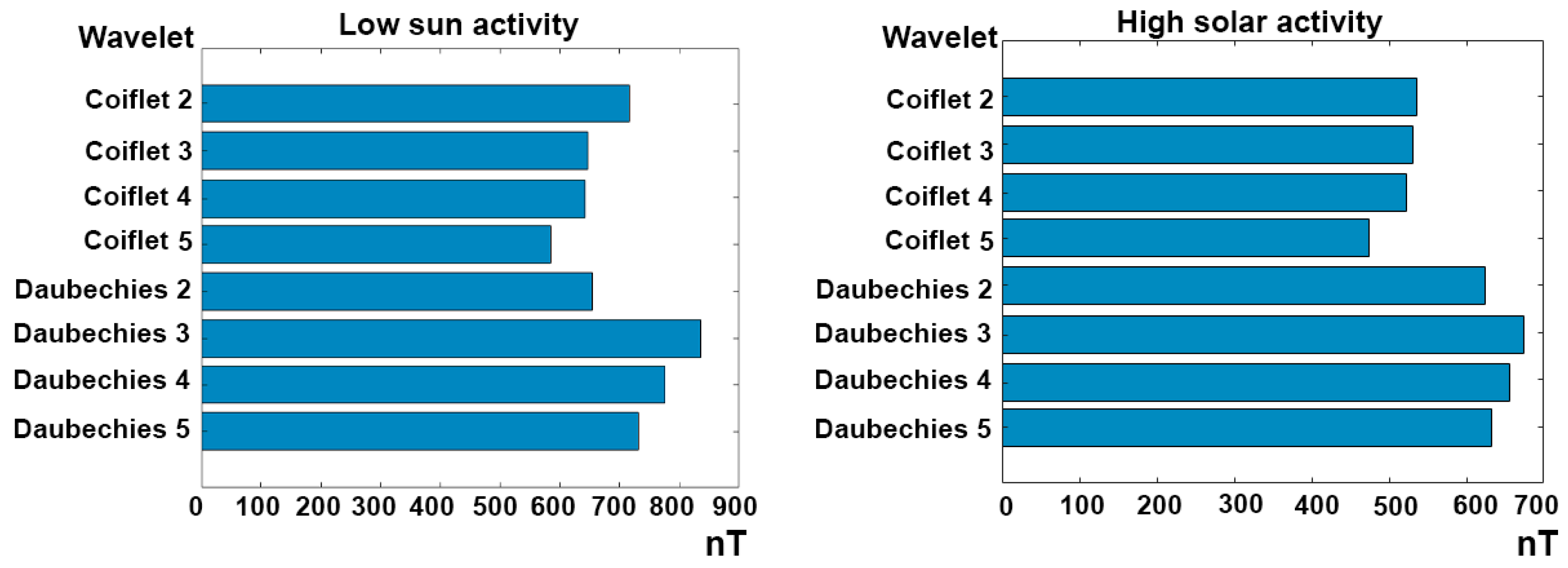
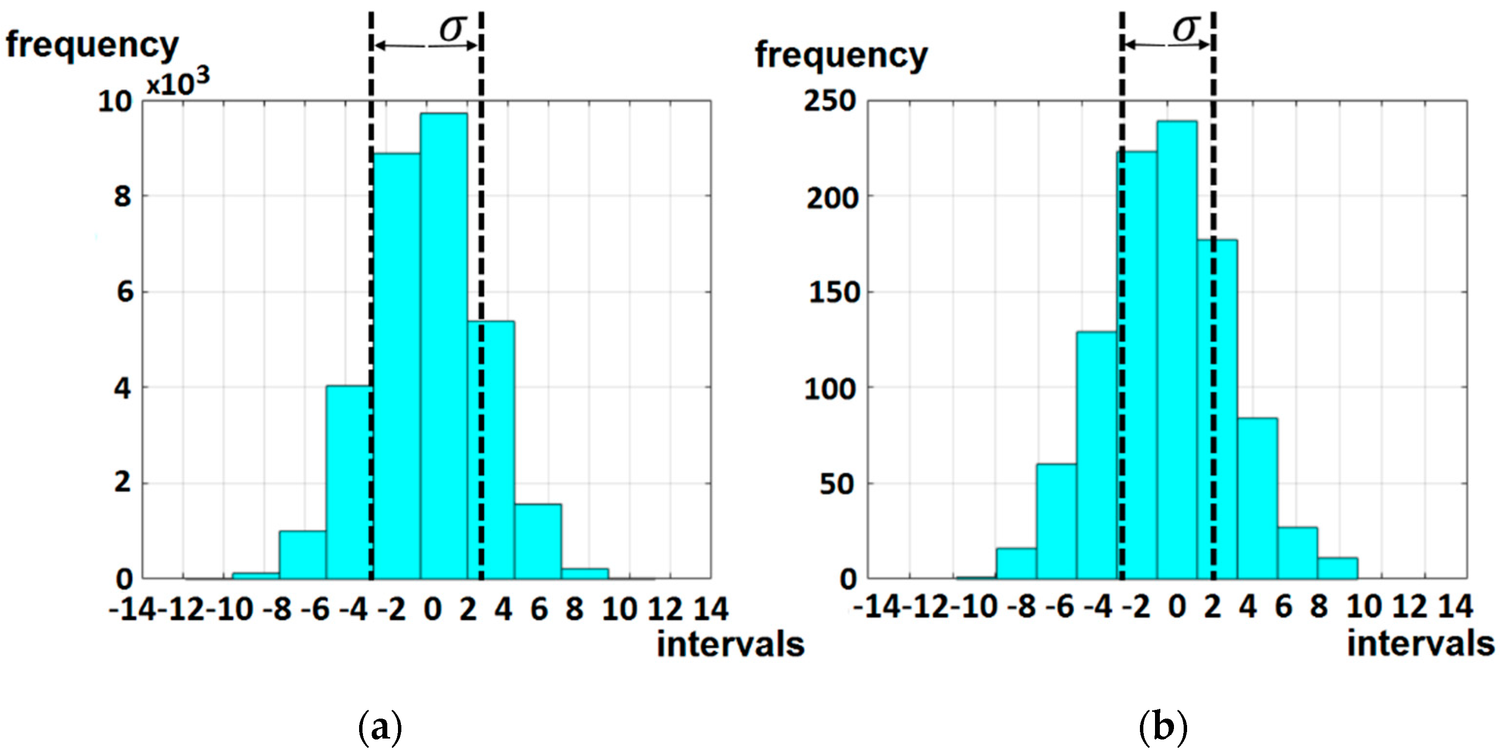
Figure 1 shows the histograms of two nodes of the wavelet packet tree, the dashed line shows the estimated σ . The results support the need to adapt the threshold to the scale. The tree constructed on the basis of the ACAS up to the 6th level using Coiflet 3 is shown in Figure 2. Geomagnetic pulsations are determined by the detailing nodes of the tree, therefore the nodes ( j i , 0 ) are not analyzed below. Table 1 and Figure 3 present the error estimation results, which show that Coiflet 5 provides the smallest losses for different periods of solar activity. The results of detection of geomagnetic pulsations using different wavelets are shown in Figure 4.
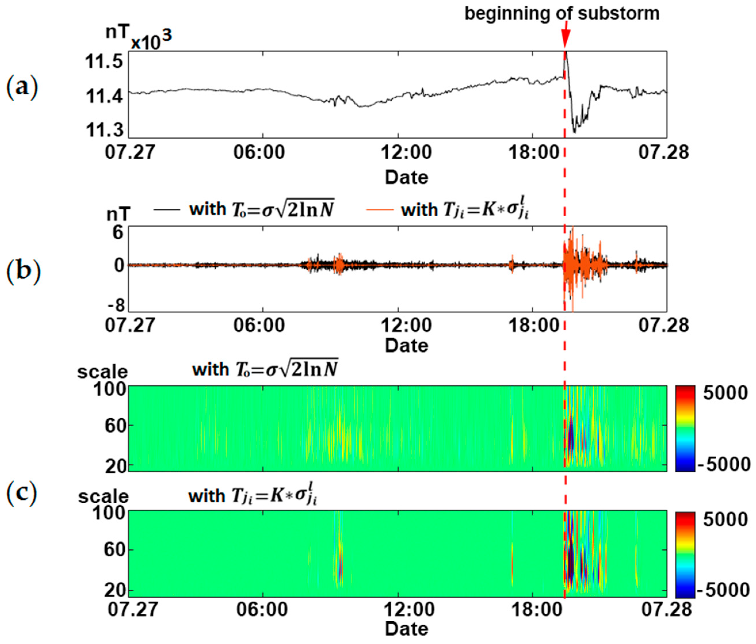
The results of risk estimates (errors of the 1st and 2nd kind) are presented in Table 2. They show that the threshold coefficient K   =   2.5 gives the best results. Risks were estimated based on statistical modeling. As a comparison, Figure 5 shows the results of the application of the threshold T о = σ 2   l n   N and the threshold T j i = K σ j i l , with K   =   2.5 . It can be seen that threshold T о , which is close to optimal one, does not allow us to suppress the noise. The results confirm the effectiveness of the proposed method.

3.2. Detection of Sporadic Features in Neutron Monitor Data

Cosmic ray dynamics are studied using neutron monitor data. Neutron monitor data represent particle counts per unit time and reflect the secondary cosmic ray intensity. In addition to the useful information, the data contain a high level of noise, including natural and human-made interferences [4]. Periodic variations correspond to the regular course and anomalous (sporadic) features characterize Forbush effect occurrences and strong ground level enhancements (GLE events). Sporadic features have different shapes and durations, and their detection is a difficult problem [4]. Of particular interest is the problem of detecting low-amplitude sporadic features that serve as predictors of magnetic storms [4].
Figure 6, Figure 7, Figure 8, Figure 9, Figure 10 and Figure 11 show the results of applying the method to the neutron monitor (NM) data of the Inuvik station (USA, [24]). Figure 6 shows the histograms of two nodes of the wavelet packet tree. The dashed line shows the estimated σ. The results are similar to geomagnetic data.
To assess the effectiveness of the proposed method, its results were compared with the results of the autoencoder method [25]. Autoencoder is a deep feed forward neural network using back propagation and unsupervised learning. The autoencoder network is described in detail in [25]. The work used undercomplete autoencoders. Minimizing the approximation error, the undercomplete autoencoders allow one to isolate dependencies in the data and to suppress noise. The logistic sigmoidal function was used as the encoder transfer function:
f ( z ) = 1 1 + e z
As the transfer function of the decoder, a linear transfer function was used:
f ( z ) = z .
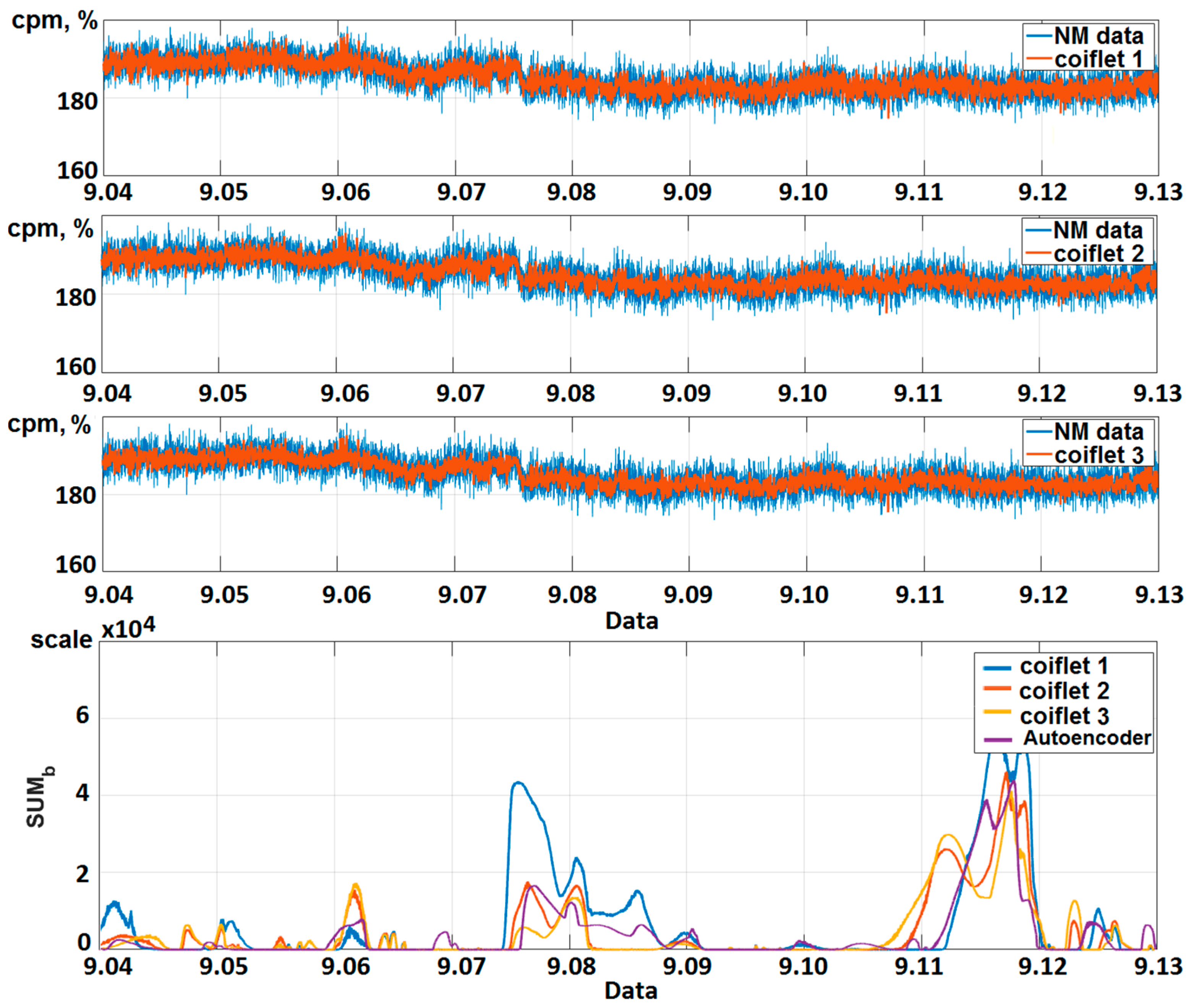
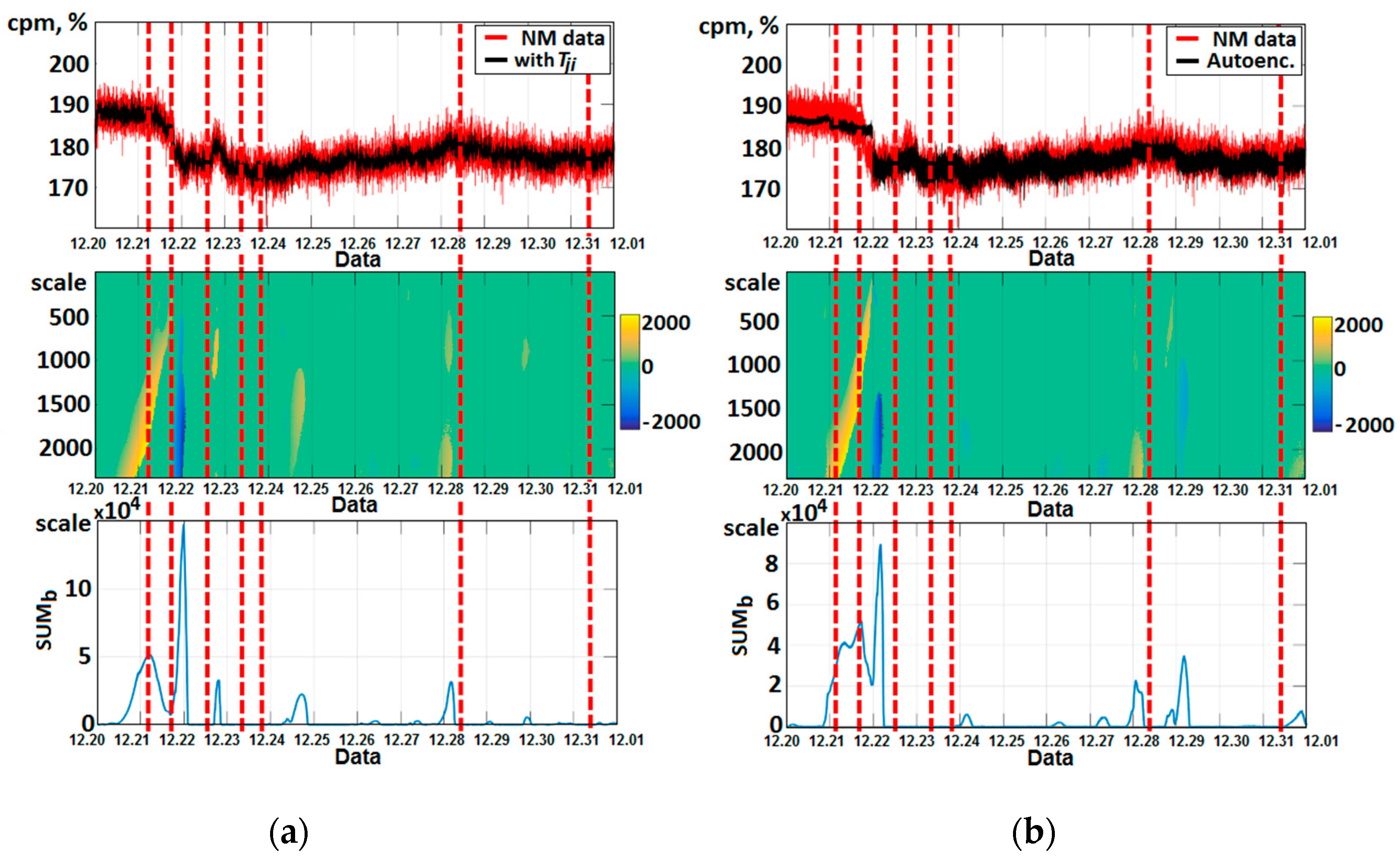
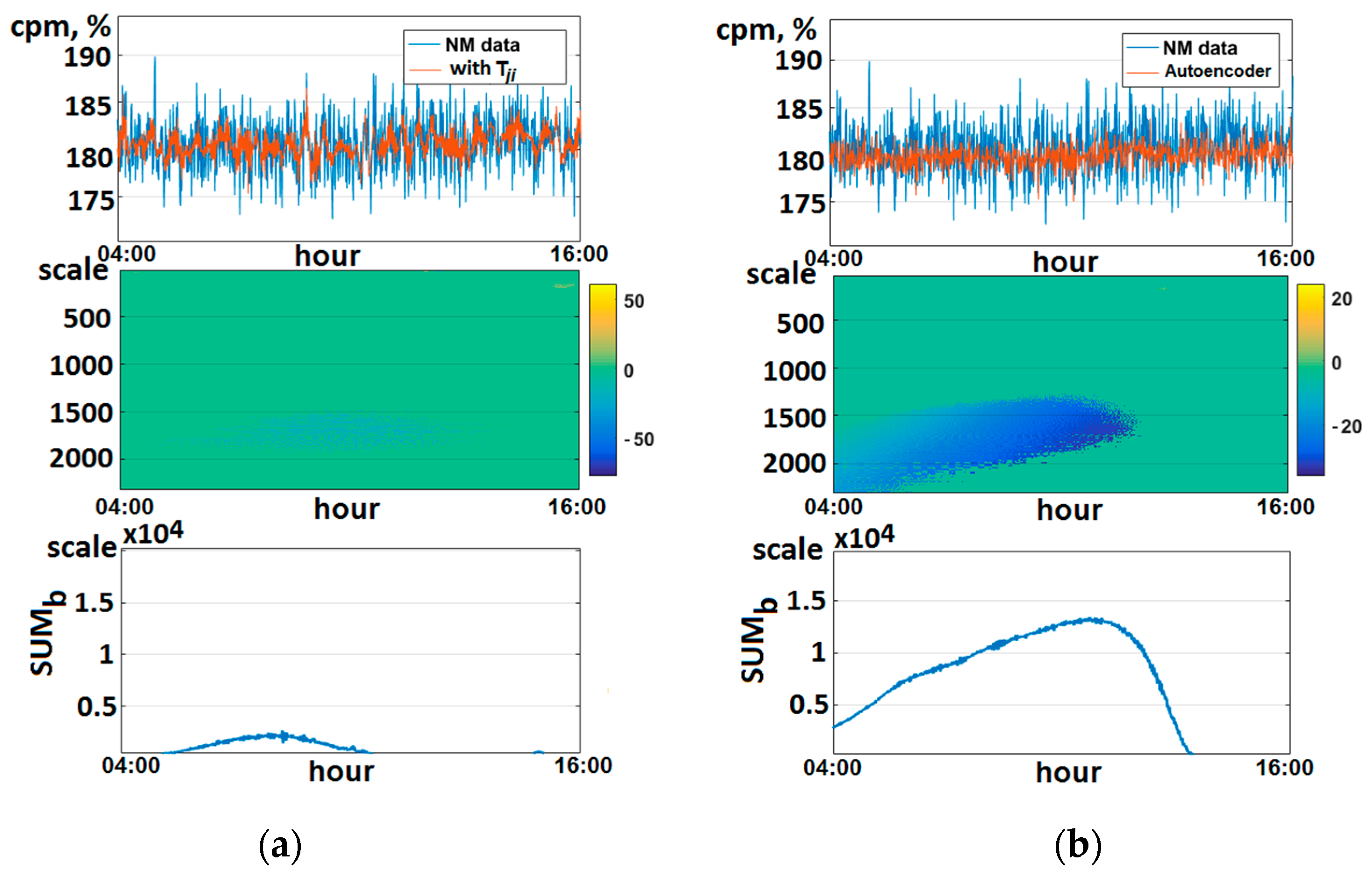
To train the network, we used NM data for 2013–2015. Figure 7 shows the results of NM data processing by different methods. The threshold T о = σ 2   ln   N , the threshold T j i = K σ j i l and the autoencoder network were used. It is clear that the threshold T о = σ 2   ln   N does not allow us to suppress all the noise. The error of network approximation increases sharply in the test data. That is associated with the effect of retraining and the need to adapt the network. The best results are obtained by the proposed method with the threshold T j i = 2.5 σ j i l . Table 3 shows the errors of different methods. Analysis of Table 3 also confirms the effectiveness of the proposed method. Figure 8 and Figure 9 show the results of detecting Forbush effects in NM data based on the proposed method and autoencoder. Data were processed sequentially. First, the data were processed based on the ACAS (algorithm for constructing an approximating scheme). Then, the anomaly detection algorithm described in Appendix A [26] was applied. Alternatively, the data were processed by the autoencoder network, then the anomaly detection algorithm was applied. Forbush effects were detected on 4, 6, 8, 10, 11, 12 September 2014 [27]. In Figure 9, the periods of Forbush effects are marked with red vertical lines. The results show that application of both the autoencoder and the proposed method makes it possible to detect anomalies. It can be seen that the Forbush effect on 22 December was successfully detected based on the proposed method (Figure 9a), and the Forbush effect on 31 December was detected by a neural network (Figure 9b). For detailed comparison of the results, Figure 10 and Figure 11 show periods of Forbush effects of different structures. Figure 10 shows the Forbush effect of a multiscale structure, which was detected by the proposed method. As the result in Figure 11 shows, the Forbush effect of a narrower spectrum was detected by the autoencoder.
Thus, the joint application of these methods increases the efficiency of the problem solution. Estimation of the efficiency of the proposed method is illustrated in Table 4. It shows that its efficiency (over 86%) exceeds that of the autoencoder neural network.

4. Conclusions

In this paper, a new method for the identification of structures of a complex signal and noise suppression based on nonlinear approximating schemes is proposed. The experimental results confirmed the effectiveness of the method for the tasks of analyzing natural data and detecting anomalies. Estimates have shown:
1. Application of the proposed adaptive threshold increases the error of nonlinear approximation, but increases the efficiency of anomaly recognition in a complex signal.
2. For signals of an a priori defined structure, a threshold close to optimal is more effective, since it provides the construction of a nonlinear approximating scheme with minimal risk. In the case of white noise, an optimal threshold can be obtained by minimizing the cost function. In addition, the use of this method allows you to control the resulting risk.
3. Comparison of the proposed method with the autoencoder neural network confirmed its high efficiency for natural signals (over 86%) and showed its effectiveness for detecting the features of a multiscale structure. However, the frequency of false alarms (error of the first kind) in the autoencoder is less than that of the proposed method. The autoencoder also detects narrow spectrum features more efficiently.

Author Contributions

Formal analysis, B.M. and A.R.; Methodology, O.M.; Project administration, O.M.; Software, B.M. and A.R. All authors have read and agreed to the published version of the manuscript.

Funding

The work was carried out according to the Subject AAAA-A21-121011290003-0 “Physical processes in the system of near space and geospheres under solar and lithospheric influences” IKIR FEB RAS.

Informed Consent Statement

Not applicable.

Data Availability Statement

Not applicable.

Acknowledgments

The authors are grateful to the institutes that support the neutron monitor stations (http://cosray.unibe.ch/, http://spaceweather.izmiran.ru/rus/fds2015.html) (accessed on 11 November 2020) and ground-based magnetometers (www.inrtermagnet.org) (accessed on 11 November 2020) the data of which were used in the work.

Conflicts of Interest

The authors declare no conflict of interest.

Appendix A

Algorithm for detection of anomalies in cosmic rays dynamics and estimation of their intensity [26].
Step 1. Continuous wavelet transform
( W Ψ f b , s ) : = | s | 1 2 + f ( t ) Ψ ( t b s ) d t ,
f L 2 ( R ) ,   s , b R ,   s 0
Step 2. Application of threshold function P T s :
P T s ( W Ψ f b , s ) = { W Ψ f b , s ,     i f     ( W Ψ f b , s W Ψ f b , s m e d , l ) T s l 0 ,   i f | W Ψ f b , s W Ψ f b , s m e d , l | < T s l W Ψ f b , s ,   i f   ( W Ψ f b , s W Ψ f b , s m e d , l ) < T s l
where W Ψ f b , s m e d , l is the median value calculated in a moving time window of length l . T s l = U σ s l is the threshold,
σ s l = 1 l k = 1 l ( W Ψ f b , s W Ψ f b , s ¯ ) 2
is the standard deviation calculated in a moving time window of length l , W Ψ f b , s is the average, U is the threshold coefficient.
Step 3. Estimation of anomaly intensity:
S U M s ( t ) = b P T s ( W Ψ f b , s ) ,
which is positive in the case of CR local increase and is negative in the case of CR local decrease.

References

  1. Perez-Sanchez, A.V.; Perez-Ramirez, C.A.; Valtierra-Rodriguez, M.; Dominguez-Gonzalez, A.; Amezquita-Sanchez, J.P. Wavelet Transform-Statistical Time Features-Based Methodology for Epileptic Seizure Prediction Using Electrocardiogram Signals. Mathematics 2020, 8, 2125. [Google Scholar] [CrossRef]
  2. Shestakov, O. Wavelet Thresholding Risk Estimate for the Model with Random Samples and Correlated Noise. Mathematics 2020, 8, 377. [Google Scholar] [CrossRef] [Green Version]
  3. Alperovich, L.; Eppelbaum, L.; Zheludev, V.; Dumoulin, J.; Soldovieri, F.; Proto, M.; Bavusi, M.; Loperte, A. A new combined wavelet methodology: Implementation to GPR and ERT data obtained in the Montagnole experiment. J. Geophys. Eng. 2013, 10, 025017. [Google Scholar] [CrossRef]
  4. Abunina, M.A.; Belov, A.V.; Eroshenko, E.A.; Abunin, A.A.; Yanke, V.G. Ring of Stations Method in Cosmic Rays Variations Research. Sol. Phys. 2020, 295, 1–20. [Google Scholar] [CrossRef]
  5. Zaitsev, A.N.; Dalin, P.A.; Zastenker, G.N. Sharp variations in the flux of solar wind ions and their response to disturbances of the earth’s magnetic field. Geomagn. Aeron. 2002, 6, 752–759. [Google Scholar]
  6. Mallat, S. A Wavelet Tour of Signal Processing; Academic Press: London, UK, 1999; p. 620. [Google Scholar]
  7. Singh, J.; Barabanov, N. Stability of discrete time recurrent neural networks and nonlinear optimization problems. Neural Netw. 2016, 74, 58–72. [Google Scholar] [CrossRef] [PubMed] [Green Version]
  8. Chui, C.K. An Introduction in Wavelets; Academic Press: New York, NY, USA, 1992; p. 264. [Google Scholar]
  9. Mandrikova, O.V.; Solovev, I.S.; Zalyaev, T.L. Methods of analysis of geomagnetic field variations and cosmic ray data. Earth Planet Space 2014, 66, 1–17. [Google Scholar] [CrossRef] [Green Version]
  10. Alperovich, L.; Zheludev, V.; Hayakawa, M. Application of a wavelet technique for the detection of earthquake signatures in the geomagnetic field. Nat. Hazards Earth Syst. Sci. 2001, 1, 75–81. [Google Scholar] [CrossRef] [Green Version]
  11. Alperovich, L.; Zheludev, V.; Hayakawa, M. Use of wavelet analysis for detection of seismogenic ULF emissions. Radio Sci. 2003, 38, 1093. [Google Scholar] [CrossRef]
  12. Cao, K.; Zeng, X. Adaptive Wavelet Estimations in the Convolution Structure Density Model. Mathematics 2020, 8, 1391. [Google Scholar] [CrossRef]
  13. Herley, C.; Kovacevic, J.; Ramchandran, K.; Vetterli, M. Tilings of the time-frequency plane: Construction of arbitrary orthogonal bases and feist tiling algorithms. IEEE Trans. Signal Proc. 1993, 41, 3341–3359. [Google Scholar] [CrossRef] [Green Version]
  14. Chen, S.; Donoho, D. Atomic Decomposition by Basis Pursuit; Technical Report; Stanford University: Stanford, CA, USA, 1995. [Google Scholar]
  15. Mallat, S.G.; Zhang, Z.F. Matching pursuits with time-frequency dictionaries. IEEE Trans. Signal Process. 1993, 41, 3397–3415. [Google Scholar] [CrossRef] [Green Version]
  16. Coifman, R.R.; Wickerhauser, M.V. Entropy-based algorithms for best basis selection. IEEE Trans. Inf. Theory 1992, 38, 713–718. [Google Scholar] [CrossRef] [Green Version]
  17. Daubechies, I. Ten Lectures on Wavelets; CBMS-NSF Lecture Notes; SIAM: Philadelphia, PA, USA, 1992. [Google Scholar]
  18. Wald, A. Statistical Decision Functions; John Wiley & Sons: New York, NY, USA; Chapman & Hall: London, UK, 1950. [Google Scholar]
  19. Donoho, D.L.; Johnstone, I.M. Ideal spatial adaptation via wavelet shrinkage. Biometrika 1994, 81, 425–455. [Google Scholar] [CrossRef]
  20. Jaffard, S. Pointwise smoothness, two-microlocalization and wavelet coefficients. Publ. Mat. 1991, 35, 155–168. [Google Scholar] [CrossRef] [Green Version]
  21. Bansal, A.K. Bayesian Parametric Inference; Narosa Publishing House Pvt. Ltd.: New Delhi, India, 2007. [Google Scholar]
  22. Kuznetsov, V.D. Space weather and risks of space activities. Space Technol. Technol. 2014, 3, 3–13. [Google Scholar]
  23. Despirac, I.V.; Kleimenova, N.G.; Gromova, L.I.; Gromov, S.V.; Malysheva, L.M. Supersubstorms during storms on 7–8 September 2017. Geomagn. Aeron. 2020, 60, 308–317. [Google Scholar] [CrossRef]
  24. Real Time Data Base for the Measurements of High-Resolution Neutron Monitor. Available online: www.nmdb.eu (accessed on 1 November 2020).
  25. Ian, G.; Yoshua, B.; Aaron, C. Deep Learning; Random House: New York, NY, USA; p. 808.
  26. Mandrikova, O.; Polozov, Y.; Fetisova, N.; Zalyaev, T. Analysis of the dynamics of ionospheric parameters during periods of increased solar activity and magnetic storms. J. Atmos. Sol. Terr. Phys. 2018, 181, 116–126. [Google Scholar] [CrossRef]
  27. IZMIRAN Space Weather Forecast Center. Catalog of Forbush Effects and Interplanetary Disturbances. Available online: http://spaceweather.izmiran.ru/rus/fds2019.html (accessed on 11 November 2020).
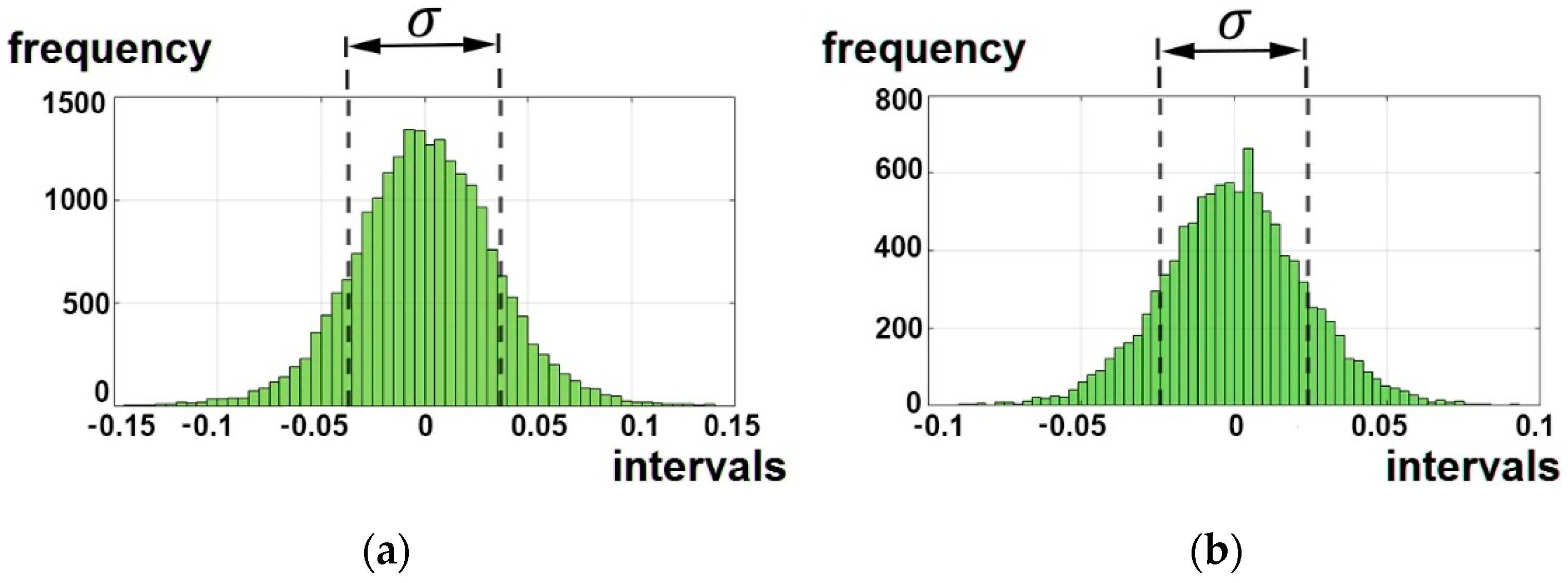
Figure 1. Histograms of tree nodes, Daubechies 3: (a) node (2, 1); (b) node (5, 1).
Mathematics 09 00737 g001
Figure 2. Constructed tree.
Mathematics 09 00737 g002
Figure 3. Estimation of the approximation error for different bases.
Mathematics 09 00737 g003
Figure 4. (a) Signal; (b,c) method application (without nodes (ji,0)).
Mathematics 09 00737 g004
Figure 5. Results with different thresholds.
Mathematics 09 00737 g005
Figure 6. Histograms of tree nodes, Coiflets 3: (a) node (2, 1); (b) node (5, 1).
Mathematics 09 00737 g006
Figure 7. Neutron monitor (NM) data processing results.
Mathematics 09 00737 g007
Figure 8. NM data processing results, the threshold used was T j i = 2.5 σ j i l .
Mathematics 09 00737 g008
Figure 9. NM data processing results (2014.03.25): (a) the proposed method, the threshold used was T j i = 2.5 σ j i l ; (b) autoencoder.
Mathematics 09 00737 g009
Figure 10. NM data processing results (2014.03.29 from 04:00 to 16:00): (a) the proposed method, the threshold used was T j i = 2.5 σ j i l ; (b) autoencoder.
Mathematics 09 00737 g010
Figure 11. NM data processing results: (a) the proposed method, the threshold used was T j i = 2.5 σ j i l ; (b) autoencoder.
Mathematics 09 00737 g011
Table 1. Estimation of the approximation error.
Wavelet, ΨNumber of Tree NodesApproximation Error, ϵ[M]
Daubechies 24457.95443552
Daubechies 34495.03347346
Daubechies 43773.25697093
Daubechies 56163.16288707
Coiflet 24277.63664436
Coiflet 34070.45379894
Coiflet 44461.81353236
Coiflet 54856.32646977
Table 2. Risks.
Table 2. Risks.
Signal/NoiseThreshold Coefficient K = 2.5Threshold Coefficient K = 1.5
Part of Detected (%)Part of False (%)Part of Detected (%)Part of False (%)
18948713
0.88174915
0.772106617
Table 3. Estimation of the approximation error.
MethodApproximation Error, ϵ[M]
Autoencoder, training310.2346
Autoencoder testing4.2870 × 105
Threshold T = σ 2   ln   N , Coiflet 17.2196 × 10⁻¹⁰
Threshold T j i = K σ j i l , K = 1 , Coiflet 1176.0616
Threshold T j i = K σ j i l , K = 1.5 , Coiflet 1273.2969
Threshold T j i = K σ j i l , K = 2.5 , Coiflet 1376.4855
Threshold T j i = K σ j i l , K = 1 , Coiflet 2177.1038
Threshold T j i = K σ j i l , K = 1.5 , Coiflet 2273.45
Threshold T j i = K σ j i l , K = 2.5 , Coiflet 2375.741
Threshold T j i = K σ j i l , K = 1 , Coiflet 3176.9381
Threshold T j i = K σ j i l , K = 1.5 , Coiflet 3274.2327
Threshold T j i = K σ j i l , K = 2.5 , Coiflet 3376.1264
Table 4. Estimation of the efficiency of the proposed method.
YearThe Number of Forbush Effects in the SignalProposed MethodAutoencoder
201398Detected: 86%Detected: 79%
Not detected: 14%Not detected: 21%
False alarm: 16 eventsFalse alarm: 11 events
201496Detected: 89%Detected: 84%
Not detected: 11%Not detected: 16%
False alarm: 12 eventsFalse alarm: 9 events
201591Detected: 84%Detected: 76%
Not detected: 16%Not detected: 24%
False alarm: 10 eventsFalse alarm: 8 events
Publisher’s Note: MDPI stays neutral with regard to jurisdictional claims in published maps and institutional affiliations.