1. Introduction
Artificial neural networks (ANNs) are a machine learning technique that is widely used as an alternative forecasting method to traditional statistical approaches in many scientific disciplines [
1], such as marketing, meteorology, finance, or environmental research, when a massive amount of data is challenging to manage.
Unlike conventional methodologies, ANNs are data-driven self-adaptive, and non-linear methods that do not require specific assumptions about the underlying model [
2]. ANNs are data-driven because they can process the available data (input) and produce a target variables vector (output) through a feed-forward algorithm. Moreover, the method is self-adaptive. In fact, a neural network can approximate a wide range of statistical models without hypothesizing in advance on any relationships between the dependent and independent variables. Instead, the form of the relationship is determined during the network learning process. If a linear relationship between the dependent and independent variables is appropriate, the neural network results should closely approximate those of the linear regression model. If a non-linear relationship is more appropriate, the neural network will automatically match the “correct” model structure. Therefore, this algorithm is suitable for approximating complex relationships between the input and output variables with a non-linear optimization [
3].
ANNs algorithms simulate how the human brain processes information through the nerve cells, or neurons, connected to each other in a complex network, within a computational model [
4]. The similarity between an artificial neural network and a biological neural network relies on the network’s acquirement of knowledge through a “learning process” [
5]. From the initial data (input), it is possible to determine the target variable (output) through the complex system of cause–effect relationships that the model discovers.
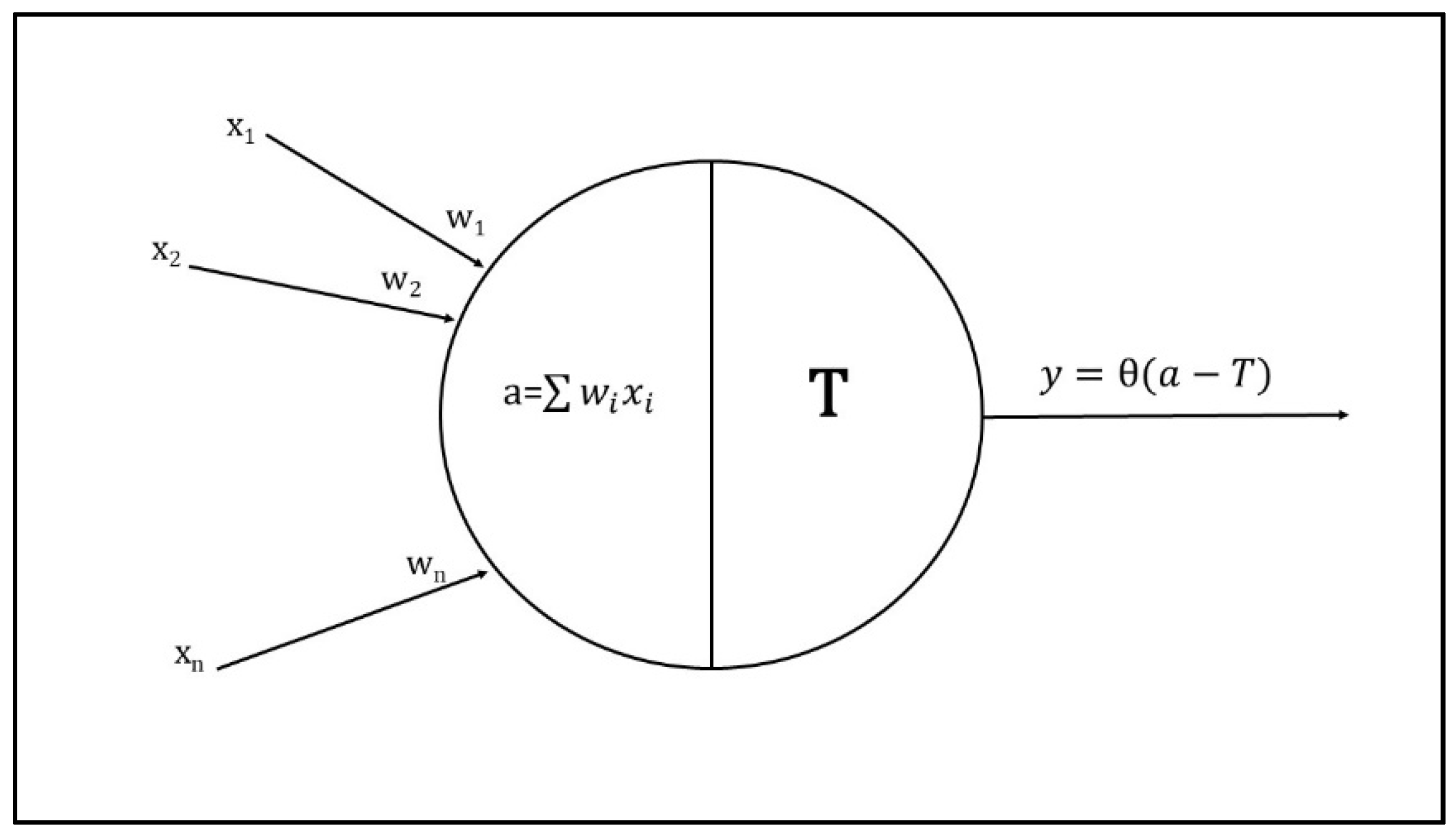
The neuron (node) is the primary processing unit in neural networks. Each artificial neuron has weighted inputs, transfer functions, and one output. An example of neural propagation is the McCulloch–Pitts model (
Figure 1), which combines its inputs (typically as a weighted sum) to generate a single output.
In this model, the inputs x
i are multiplied by the weights w
i, with w
0 as bias. Bias shifts the activation function by adding a constant to the input to better fit the data prediction. Bias in neural networks can be thought of as analogous to the role of a constant in a linear function, whereby the constant value transposes the line: without w
0, the line would go through the origin (0, 0), and the fit could be poor. If the weighted sum of the inputs “a” overcomes a threshold value T, neurons release its output y, which is a function of (
a-T). In other words, the arriving signals (inputs), multiplied by the connection weights, are first summed and then passed through an activation function (θ) to produce the output [
6]. A unit feeds its output to all the nodes on the next layer, but there is no feedback to the previous layer (feed-forward network). Weights represent the system memory and indicate the importance of each input neuron in the output generation processing. The activation function is used to introduce non-linearity in the network’s modeling capabilities [
7]. Activations are typically a number within the range of 0 to 1, and the weight is a double, e.g., 2.2, −1.2, 0.4.
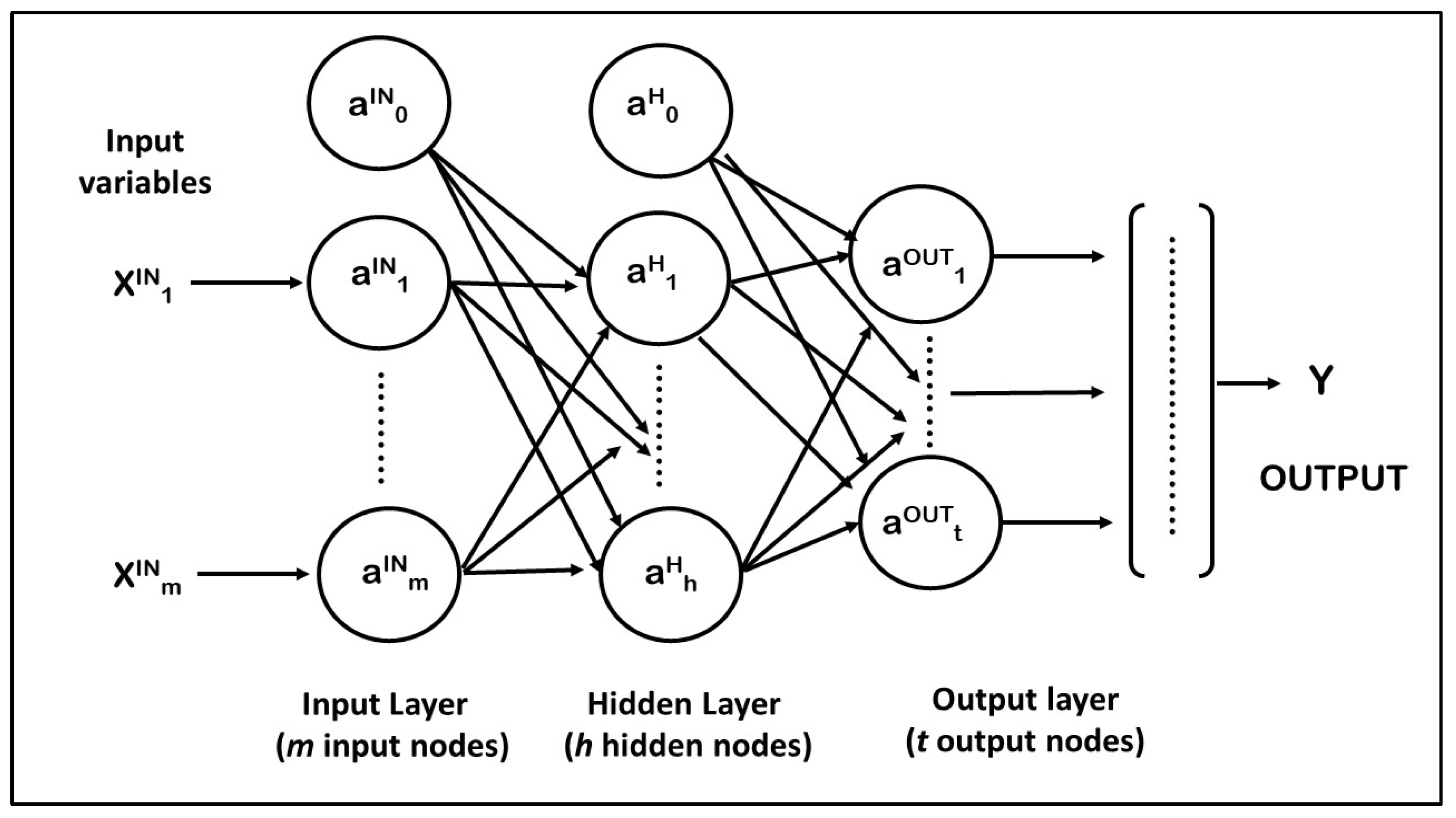
In a neural network, there are many parameters for building a model. It is possible to change the number of layers, the number of neurons for each layer, the type activation function to use in each layer, the training duration, and the learning rule.
The optimization of neural network architecture is a reccurring topic of several studies. Generally, the different approaches regard empirical or statistical methods to analyze the effect of an ANN’s internal parameters, choosing the best values for them based on the model’s performance [
8,
9], e.g., through the notions from Taguchi’s design of experiments [
10], or hybrid methods composed of a feed-forward neural network and an optimization algorithm to maximize weights and biases of the network [
11,
12]. Other authors have compared the performance of different feed-forward and recurrent ANNs architectures, using the trial-and-error method to determine these parameters’ optimal choice [
13,
14]. For each of the architectures, the activation functions, the number of layers, and the number of neurons are found employing a trial-and-error procedure, as the best compromise between estimation accuracy, time of training, and the need to avoid training overfitting. A different optimization approach adds and/or removes neurons from an initial architecture using a previously specified criteria to indicate how the ANN performance is affected by the changes [
15]. The neurons are added when training is slow or when the mean squared error is larger than a specified value. Simultaneously, the neurons are removed when a change in a neuron’s value does not correspond to a change in the network’s response or when the weight values associated with this neuron remain constant for a large number of training epochs. Several studies have proposed optimization strategies by varying the number of hidden layers and hidden neurons through the application of genetic operators (GA) and evaluation of the different architectures according to an objective function [
16,
17]. This approach considers the problem as a multi-objective optimization, and the solution space is the collection of all the different combinations of hidden layers and hidden neurons. Given a complex problem, a genetic algorithm (GA) is developed to search the solution space for the “best” architectures, according to a set of predefined criteria. A GA is an artificial intelligence search metaheuristic derived from the process of biological organism evolution [
18]. The GA is often preferred to conventional optimization algorithms due to its simplicity and high performance in finding the solutions for complex high-dimensional problems. The ability to handle arbitrary objectives and constraints is one of the advantages of the genetic algorithm approach [
19]. Unlike the traditional optimization method, GA uses probabilistic transition rules instead of using deterministic rules. It works by coding the solution instead of using the solution itself. Moreover, it works with a population of solutions instead of a single solution. However, even if GA requires less information about the problem, designing an objective function and getting the proper representation can be difficult. In addition, GA does not constantly assess a global optimum, and it can produce a quick response time only in the case of a real-time application [
20].
In this study, because of the large number of variables and factors to optimize, despite the advantages of GA as an optimization method, it has been preferred to take a strategy of reduction of the number of experiments to conduct, using Taguchi’s factorial Design of Experiment (DoE) to identify the best architecture (number of hidden layers, number of hidden neurons, choice of input factors, training algorithm parameters, etc.) of a Multi-Layer Perceptron model, considering as a case of study an environmental problem of pollution characterization. Taguchi’s method is an important tool for robust DoE. It represents a simple and systematic approach to optimize the design, maximizing performance and quality, and minimizing the number of experiments, reducing the experimental design cost [
21]. The main reason to choose the Taguchi method instead of other optimization algorithms (such as GA) is its capability to reduce the time required for experimental investigation and to study the influence of individual factors to determine which factor has more influence and which has less. Orthogonal arrays, the principal tool on which the method is based, accommodate many design factors simultaneously, obtaining different information for each test, even when applying the most straightforward deterministic statistical techniques. In this paper, the optimization of a shallow network (§ 2.1.1) has been considered. Many authors have implemented the Taguchi method also for optimization of a deep neural network (DNN) [
22,
23]. A DNN is a net with multiple layers between the input and output layers. Deep learning has demonstrated an excellent performance to solve pattern recognition problems, such as computer vision, speech recognition, natural language processing, and brain–computer interface [
24]. At the same time, it is less often used as a forecasting method.
3. Results
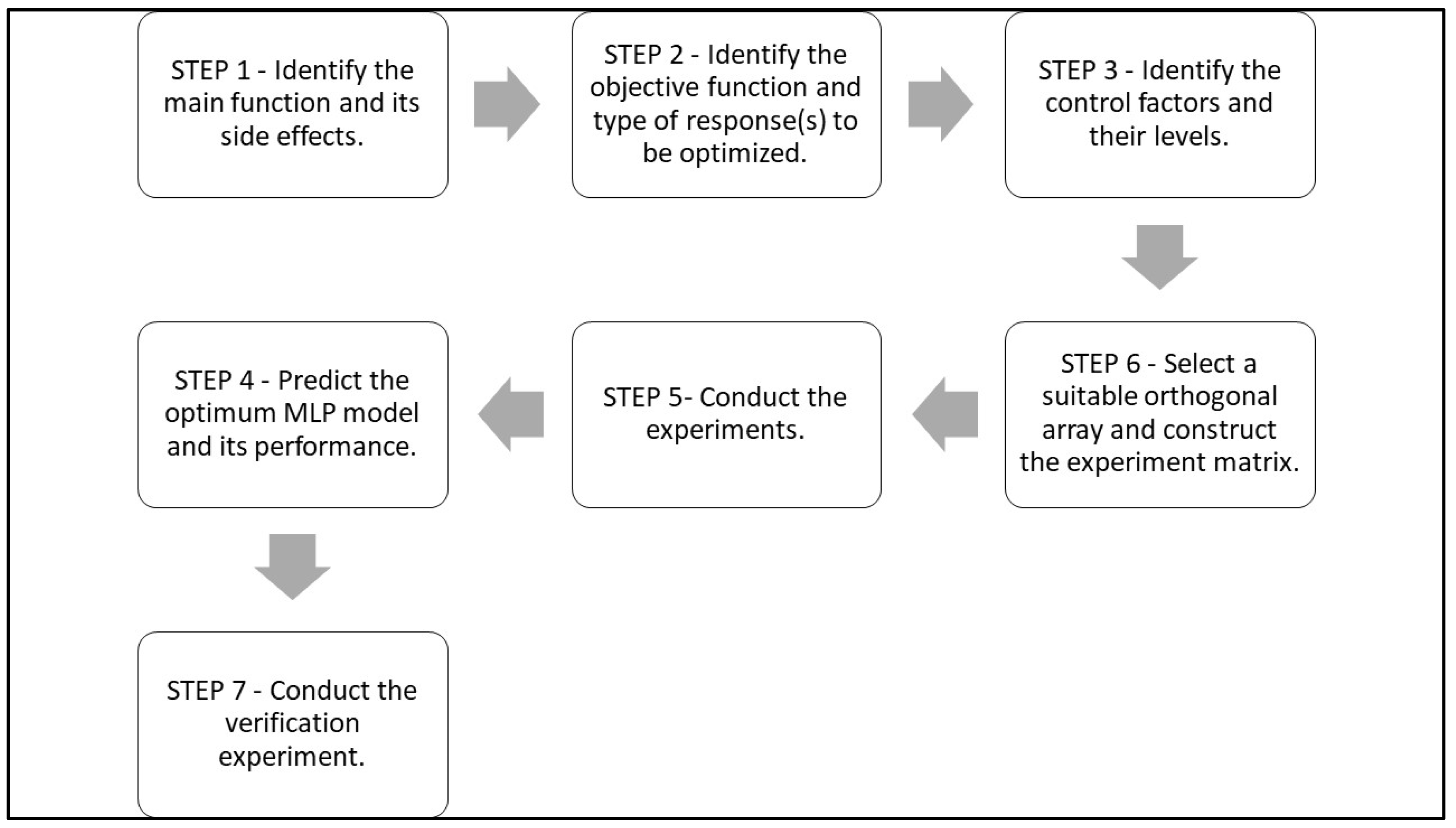
According to these steps, a series of experiments has been carried out. The procedure has been illustrated in the following subsections.
3.1. Step 1. Identify the Main Function and Its Side Effects
The optimization of ANNs’ predictive capability has been considered as the main function. No side effects have been recorded. Before proceeding to the following steps, it is necessary to detect all the factors influencing the network performance, identifying them as signal (or control) and/or noise factors [
50]. Signal factors are the system control inputs, while noise factors are typically difficult or expensive to control. In this analysis, all the considered factors are controllable in the model; they have been classified as “signal factors” and none were classified as “noise factors”.
3.2. Step 2. Identify the Objective Function and Type of Response(s) to Be Optimized
The index
R2, one of the three performance measures (§ 2.1.4), was chosen as the objective function or response variable to be maximized. The target value of
R2 has been set to 0.70 or more. Taguchi recommends using a loss function to quantify a design’s quality, defining the loss of quality as a cost that increases quadratically with the deviation from the target value. Usually, the quality loss function considers three cases: nominal-the-best, smaller-the-better, and larger-the-better [
51], corresponding to three types of continuous measurable responses to be optimized [
52]:
Target-is-the-best (TTB) response, when the experiment’s objective is to achieve a desired target performance for the response variable.
Smaller-the-better (STB) response, in which the desired target is to minimize the response variable.
Larger-the-better (LTB) response, when the experiment’s objective is to maximize the response within the acceptable design limits.
According to this scheme, in this analysis, R2 qualifies as an LTB response.
To quantify the output quality, Taguchi suggests that the objective function to be optimized is the signal/noise ratio (
S/N Ratio) [
53], which is a logarithmic function of the response variable with a different trend depending on the type of response. An objective function of an LTB response is calculated assuming the following formula:
where
n is the number of the experiments or runs in a Taguchi design, and
y is the response value in the run
i. The level indicated the best experimental results obtained by the calculation of average
S/N ratio for each factor and the optimal level of the process parameters with the largest
S/N ratio.
3.3. Step 3. Identify the Control Factors and Their Levels
The signal (or control) factors and their levels (§ 2.1) are shown in
Table 1.
A parametric set of seven variables of an MLP model has been considered and in detail listed below:
Number of samples. The experiment can detect the minimum number of sample units sufficient for the network to learn. In a 64-sample database, three levels of this factor have been fixed: 10, 30, and 50 units.
Input scaling rule. Two levels are corresponding to the different criteria to scale input data (§ 2.3):
- (a)
normalization, using the formula
- (b)
standardization, using the formula
Training rate (%): three levels of percentage have been considered for computing the size of the training set (test set): 60% (40%), 70% (30%), and 80% (20%).
Activation function of hidden and output nodes: as mentioned above (§ 2.2), two levels have been chosen for the activation function of the hidden nodes (sigmoid and hyperbolic tangent), and three levels for the activation function of output nodes (identity function, sigmoid, and hyperbolic tangent).
Number of hidden layers: to determine if a deep network has better predictive performance, two levels of this factor have been considered: one or two hidden layers, as allowed by Neural Network function in IBM-SPSS.
Epochs. The training process duration has been set to three levels: 10, 10,000, and 60,000 epochs.
3.4. Step 4. Select a Suitable Orthogonal Array and Construct the Experiment Matrix
A full factorial design considers all input factors at two or more levels each, whose experimental units take on all possible combinations of these levels across all such factors. This experiment allows studying each factor effect on the response variable: if there are k factors each at two levels, a full factorial design has 2k runs. Thus, for seven factors at two or three levels, it would require many experiments (27 or 37) to be carried out, and too many observations to be economically viable, as stated above (§ 3).
Taguchi suggested a particular method using the orthogonal array with fewer experiments to be conducted to resolve this problem. The degrees of freedom (DoF) have to be calculated, considering one DoF for the mean value to select an adequate orthogonal array, and for each factor, the number of levels less 1. Thus, the degrees of freedom of this design are 12 (
Table 2), and the most suitable orthogonal array (OA) is L
12 (
Table 3):
Therefore, a total of twelve experiments have been carried out.
3.5. Step 5. Conduct the Experiments
By the OA L
12, each experiment has been conducted two times (24 runs in total), corresponding to 12 MLP models whose
R2,
RMSE, and
MAE in the training and test set have been calculated in each run.
Table 4 shows the measured values of response variable
R2, the mean of
R2 in each run, and the
S/N ratio obtained from each trial’s different networks.
3.6. Step 6. Predict the Optimum MLP Model and Its Performance
Thus, according to the Taguchi approach, two objective functions are optimized by larger-the-better criterium (§ 2.2.1): the mean of
R2 calculated in each run and the signal/noise ratio (
S/N Ratio). A standard approach for multi-response optimization is to identify one of the response variables as primary considering it as an objective function and other responses as constraints [
54]. Several methods of multiple response optimization have been proposed in the literature. Among them, the utilization of the desirability function is the most efficient approach [
55]. In the desirability function analysis (DFA), each response is transformed into a desirability value d
i, and the total desirability function D, which is the geometric mean of the single d
i, is optimized [
56]. Desirability D is an objective function that ranges from 0 to 1. If the response is on target, the desirability value will be equal to 1, and DFA will not maximize the desirability value. When the response falls within the tolerance range but not on the desired value, the corresponding desirability will be between 0 and 1 [
57]. As the response approaches the target, the desirability value will become closer to 1.
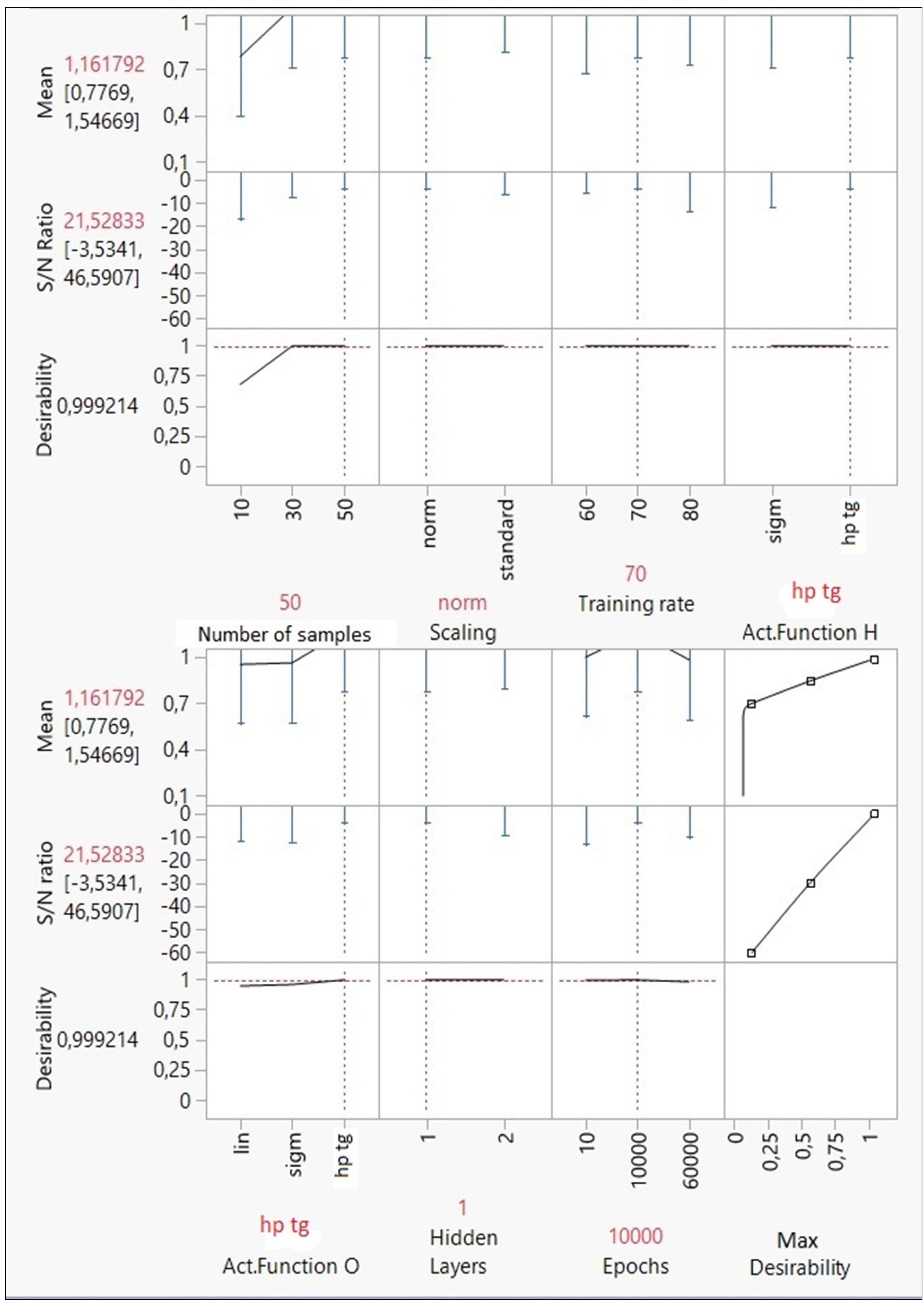
According to the desirability function analysis, the optimal combination of MLP network parameters has been obtained (
Figure 5).
Optimal response and factor values are displayed in red. The desirability function is very close to 1 (0.999214), and the tolerance interval for the
S/N ratio and mean is [−3.54, 46.6] and [0.78, 1.55], respectively. The best architecture’s features set to maximize the predictive capability of the MLP model is shown in the following outline (
Table 5).
Taguchi results are analyzed in detail below:
Number of samples: at least 50 samples are required to obtain an optimal model. Thus, a small number of units could cause unbiased predictions.
Input scaling rule: the normalization of input variables produces better results than the standardization rule.
Training rate (%): in an optimal MLP model, the training set must consider 70% of database units. Thus, the test set represents the remaining 30%.
Activation function of hidden and output nodes: the best activation function is the hyperbolic tangent for both hidden and output nodes.
Number of hidden layers: according to Taguchi’s design, a deep network is not the best solution for this analysis; one hidden layer has been more than enough to optimize the forecasts.
Epochs: the model accuracy has been determined in 10,000 epochs.
3.7. Step 7. Conduct the Verification Experiment
A new experiment (optimal network) has been carried out to compare its results with those obtained from the first MLP model (default network) (§ 2.2). In addition, to make a homogeneous comparison, a new default model has been built using the same 50 samples of the optimal net. Both new models have been an MLP feed-forward network based on 10 inputs, three hidden nodes in one layer, and one output. The architecture’s parametric set and performance indicators of three networks (MLP
def1, MLP
def2, and MLP
opt) are summarized as follows (
Table 6).
By analyzing the MLPdef1 and MLPdef2, the best solution is to consider a higher number of samples increasing performance in case of an arbitrary choice of architecture parametric set. However, the optimal model MLPopt, in which the original dataset has been normalized, has produced, with a longer training time, more reliable predictions than MLPdef1: the RMSE and MAE values (in training and test sets) are lower, and R2 is 0.93.
Therefore, through the Taguchi approach, it has been possible to find the best design to improve an MLP model performance.
In environmental analysis, relationships between organic and inorganic micro-pollutants are connected to the sampling site’s geochemical and lithological properties. Thus, this optimal MLP model is site-specific and the parametric set determined by the Taguchi method is not valid in different locations. For this reason, in various polluted areas, it is necessary to create a new application of the approach to evaluate a best-performing network.
4. Conclusions
The selection of the parametric set of a neural network model is a very challenging issue. A random choice of an MLP’s design could compromise the reliability of the network. In this paper, Taguchi’s approach for the optimal design of shallow neural networks has been presented, considering an application of the ANNs algorithm in an environmental field, to characterize a polluted soil. Different turning experiments were conducted considering the various combinations of seven architecture parameters (number of samples, scaling, training rate, the activation function of hidden and output nodes, number of hidden layers, and epochs). The optimum levels of parameters have been identified by the desirability function analysis (DFA).
The model so built is another shallow network that is able to produce more reliable predictions through a smaller dataset than the original and a longer training time. The original dataset has been preferred to be normalized than standardized. A hyperbolic tangent has proved to be the best form of the activation function for both hidden layers and output units.
Several benefits can arise from using this method to optimize an ANN’s architecture. Firstly, this methodology is the only known method for neural network design that explicitly considers robustness as a significant design criterion. This capability will improve the quality of the neural network designed. Secondly, using the methodology, several parameters of a neural network can be considered simultaneously in the optimization process, evaluating the impact of these factors of interest concurrently. Finally, the Taguchi method is not strictly confined to the design of back-propagation neural networks. Thus, this methodology will allow the rapid development of the best neural network to suit a particular application.
In environmental analysis, this method cannot be generalized since the relations between input and output variables analyzed by the network are affected by various exogenous factors that are difficult to control. Therefore, every analysis requires a new application of the Taguchi method to determine a more performing model. Then, the optimal model can be used for further analysis.


