Abstract
Fractional calculus-based differential equations were found by previous studies to be promising tools in simulating local-scale anomalous diffusion for pollutants transport in natural geological media (geomedia), but efficient models are still needed for simulating anomalous transport over a broad spectrum of scales. This study proposed a hierarchical framework of fractional advection-dispersion equations (FADEs) for modeling pollutants moving in the river corridor at a full spectrum of scales. Applications showed that the fixed-index FADE could model bed sediment and manganese transport in streams at the geomorphologic unit scale, whereas the variable-index FADE well fitted bedload snapshots at the reach scale with spatially varying indices. Further analyses revealed that the selection of the FADEs depended on the scale, type of the geomedium (i.e., riverbed, aquifer, or soil), and the type of available observation dataset (i.e., the tracer snapshot or breakthrough curve (BTC)). When the pollutant BTC was used, a single-index FADE with scale-dependent parameters could fit the data by upscaling anomalous transport without mapping the sub-grid, intermediate multi-index anomalous diffusion. Pollutant transport in geomedia, therefore, may exhibit complex anomalous scaling in space (and/or time), and the identification of the FADE’s index for the reach-scale anomalous transport, which links the geomorphologic unit and watershed scales, is the core for reliable applications of fractional calculus in hydrology.
1. Introduction
Transport of materials in Earth systems can exhibit scale-dependent dynamics in anomalous diffusion, since the functions affecting non-Fickian transport may vary, interact, and/or compete in a wide range of spatiotemporal scales and result in complex mobilization and/or retention of materials in natural geomedia (e.g., soil, slopes, rivers, and aquifers) [1]. For example, pollutant transport in the hyporheic zone (which is the interface between surface water and groundwater containing at least 10% surface water) exhibits strong scaling behaviors varying from geomorphologic unit to watershed scales [2]. Although studies on stream transport (mass and chemical) in the last three decades have made significant contributions toward better understanding of mechanisms and hydro-biogeochemical implications of hyporheic flow and transport processes [3,4,5], there remains a lack of multi-scale mathematical models that can reliably quantify pollutants and sediment dynamics in streams across multiple scales. The same challenge persists for dissolved contaminants transport in subsurface water (i.e., water in saturated porous or fractured media), which has remained a research topic in subsurface stochastic hydrology for more than four decades [6,7,8,9] and has motivated this study.
The fractional-order partial-differential equations (FPDEs) reviewed extensively by Metzler and Klafter [10] provide a set of promising tools to quantify dynamics of pollutants transported in streams and aquifers because of the following three reasons. First, the following fractional advection-dispersion equation (FADE) built upon fractional calculus was found to be applicable in capturing non-Fickian dispersion in complex media, including flow/transport in geomedia, which typically result in non-Fickian or anomalous behavior due to the multi-scale intrinsic physical/chemical heterogeneity of the media [11]:
where P [ML−3] is the material density, the symbol represents the Caputo time-fractional derivative with order [dimensionless] (0 < γ ≤ 1), [dimensionless] (1 < ≤ 2) is the index of the (positive) Riemann–Liouville space-fractional derivative, V [LT−1] is the average flow velocity, D [LαT−1] is the effective dispersion coefficient, and = 1 [Tγ−1] is used here for unit conversion (so that velocity V can have the commonly used dimension). Here, the Riemann–Liouville space-fractional derivative is needed since the corresponding FPDE on a bounded domain governs a well-defined stochastic process (while the bounded value problem for the FPDE with the Caputo space-fractional derivative generates negative solutions) [12,13]. Second, the space-nonlocal FADEs with a space-fractional derivative can capture super-diffusion (which represents fast displacement with the plume variance growing faster than linear in time) driven by hydrologic mechanisms including local-scale river turbulence, large-scale flooding, and other preferential flow paths, even though super-diffusion has been consistently ignored by current time-nonlocal transport models in hydrology [14]. Notably, the FADE (1) uses the one-side space-fractional derivative because the fast displacement for pollutant particles is usually one dimensional (from upstream to downstream) in geomedia (meaning that the two-side FPDEs are not appropriate for modeling typical hydrologic processes). Third, the time-nonlocal FADEs with a time-fractional derivative can simulate sub-diffusion due to chemical/physical sorption/desorption and/or retention of pollutants in geomedia [15].
Geomedia’s intrinsic physical/chemical heterogeneity can evolve across scales, and materials (such as sediment, colloids, nutrients, and heavy metals) may move continuously from lower to higher scales before becoming trapped or degrading. One of the main challenges of FPDEs in Earth sciences, therefore, is how to develop and apply the FPDEs to quantify anomalous transport in geomedia over a broad spectrum of scales, although the FADEs with constant parameters (including both the dispersion coefficient and the fractional derivative index) were found to be applicable in fitting anomalous transport in geomedia at a fixed scale; see the extensive review in Zhang et al. [16,17]. The other challenge is that, although fractional calculus has been introduced into hydrology and Earth sciences communities for over two decades [18], the in-depth integration of hydrologic/hydrogeological mechanisms and fractional-derivative models is rather rare, which significantly limits further applications of FPDEs in Earth sciences.
This study developed and demonstrated a technique to simulate anomalous transport at various scales using the FADEs. The rest of this work is organized as follows. Section 2 proposes a hierarchical method using multi-level FADEs to capture scale-dependent transport in the river corridor based on the physical and chemical heterogeneity of the system. Section 3 checks the applicability of the proposed FADE framework by simulating bed sediment and the heavy metal moving in real-world streams at a wide range of scales. Section 4 discusses the model feasibility and the scale-dependent FADE index by conducting Monte Carlo simulation of pollutant transport in a saturated fracture medium. Section 5 draws the conclusions. Hence, this study provides a complete picture for the theory and application of FADEs when modeling anomalous transport in the complex river corridor.
2. Hierarchical Method Using Multi-Level Fractional-Derivative Models
2.1. Multi-Scale Modeling, Anomalous Transport, and Classical Models
Our development of multi-scale models follows knowledge gained since 1962, when the concept of “multiscale” was first proposed by Tetnev in the discipline of Radio Engineering and Electronic Physics in the USSR. First, to integrate partial-differential equations at different scales, two basic approaches, the hierarchical method and the hybrid method, have been used [19,20]. The hierarchical method starts from the smallest scale, yielding results used as an input to the next scale [21], while the hybrid method allows concurrent simulations at different levels [22]. We selected the hierarchical method since it is computationally much more efficient than the hybrid method [23]. In addition, it may not be necessary to build detailed, smaller-scale processes in a larger-scale model using the FPDE, since the FPDE, theoretically and mathematically, represents the scaling limit of the sub-grid process and therefore is an “upscaling” model [24]. Second, the transfer of essential information between scales, which is usually from a lower to a higher level, or the so called “upscaling”, can be performed by taking average, integral, aggregation, or best fit for parameters [25]. In this study, the FPDE is developed for each scale, and the main information at a lower scale (which contains statistics of the essential microscopic features) can then be conveyed to the higher scale. Third, subgrid-scale variability in subsurface properties and hydro-biogeochemical processes has a significant impact on the grid-scale transport dynamics and should be represented within macroscopic models [26]. This can be done by the FPDE, which can efficiently capture non-Fickian dispersion and upscale transport kinetics without the need to map subgrid heterogeneity.
We classify the movement of pollutants in streams into three distinct spatial scales (Table 1), following the arguments in Boano et al. [2]: (a) the geomorphologic unit scale, consisting of specific bedforms such as ripples/dunes, and alternate/meander bars (in length of 10−1~100 m); (b) the reach scale (101~103 m), where most field tests were conducted; and (c) the watershed scale (>103 m), which is critical for aquatic ecosystems.

Table 1.
Properties and standard models for pollutants moving at three representative scales in streams.
Different models and strategies may be needed to capture pollutant transport at the three scales. For example, process-based physical models had been developed for the geomorphologic unit scale transport (such as the classical, well-known advective pumping model [29,30]), where the detailed sedimentological and geomorphological characteristics of the stream-aquifer system are represented. These process-based models, however, cannot be expanded to the reach or watershed scale, since the local-scale heterogeneity cannot be exhaustively mapped, motivating the development of phenomenological models such as the FPDE. Although various models differing greatly in the spatial scales they represent have been proposed (see the extensive review by Boano et al. [2]), no single or unified framework has been recognized so far for pollutant transport at all scales in streams.
The following transient storage model (TSM), initially built by Bencala and colleagues [31,32], had been widely applied to characterize non-reactive, reversible kinetic sorption of heavy metals to sediments in the transient storage zone:
where C and Cs [ML−3] denote the chemical concentration in the main channel and the storage zone, respectively; [T−1] is the rate constant for mass exchange between stream and the storage zone; A and AS [L2] are the stream and storage-zone cross-sectional areas, respectively; and V and D are the same as those in the FADE (1) (the medium here is the open channel). The finite-size, single storage zone can be separated into the streambed and the hyporheic zone by adding one more governing equation in (2). The TSM (2) is the best-known phenomenological model for the stream-aquifer system. Implementation software and variants of the TSM (1) include the popular software OTIS/OTEQ [33,34] and the geochemical submodels MINTEQ and MINEQL [35,36]. If , then there is no mass exchange or storage zone, and the TSM (2) reduces to the classical advection-dispersion equation (ADE) for conservative solutes moving in a homogeneous system.
Our view of watershed hydro-biogeochemical functions can be expressed by three essential characteristics for pollutant dynamics: (a) multi-scale processes, (b) non-stationary evolution at the reach and watershed scales, and (c) anomalous dynamics at almost all spatial scales. None of these real-world processes can be effectively addressed by traditional models such as the TSM (2) or its variants such as the two-component nutrient spiraling model (NSM) [37,38] because of the following reasons. First, the TSM (2) and its variants were built for the reach scale process and, thus, cannot upscale or downscale kinetics for pollutants moving over a broad spectrum of scales in streams. Second, these models cannot capture non-stationary kinetics, such as temporal dynamics varying from day to years. Third, they assume a single mass exchange rate and Fickian diffusion, and therefore cannot effectively model anomalous transport. Particularly, the single rate coefficient assumed by these classical models results in the exponential residence time direction (RTD) for pollutants in the river corridor, eliminating the other types of RTDs such as the (truncated) power-law distribution recommended by various researchers [39,40,41]. The exponential RTD causes the fast decline of the pollutant mass at late times for an instantaneous input, which, however, cannot explain the slow decline or persistent contamination well-documented in hydrology [42].
2.2. Development of FADEs for Multi-Scaling Transport in the River Corridor
Faithful modeling of contaminant dynamics affected by hydrologic and biogeochemical functions in streams is an important goal that has not yet been achieved in sufficient detail, even after decades of effort. The next-generation physical models, whose rigorous development can be inspired and improved by the recent advances in FPDEs, are needed to accurately elucidate hydrologic and biogeochemical processes and quantity multi-scale, non-stationary, and anomalous diffusion of pollutants in streams. In this section, we propose the general FADE for mixed super- and sub-diffusion for reactive pollutants transport in streams at each scale, while the model itself can be simplified in practical applications such as non-reactive and sub-diffusive only transport models for sediments moving along the riverbed (shown in Section 3.1).
2.2.1. Geomorphologic Unit Scale: Fixed-Index FADE for Stable Anomalous Dynamics
Geomorphologic unit scale is practicably applicable for studying hyporheic exchange since the measurable flow field provides a fixed domain for evaluating pollutant transport dynamics. Assuming that the probability density function (PDF) of random displacement and waiting times for pollutant particles follow the tempered stable densities, we propose the fixed-index FADE to model anomalous pollutant transport in rivers at the geomorphologic unit scale:
where β [Tγ−1] is the capacity coefficient describing the mass ratio between the adsorbed and mobile pollutants in equilibrium; the symbol represents the Caputo type, tempered, time-fractional derivative with the temporal truncation parameter [T−1] (whose inverse defines the maximum residence time) [40]; [L−1] is the truncation parameter in space; and denote the spatially averaged velocity and dispersion coefficient, respectively; stands for the vertical direction (pointing to the hyporheic zone); and and [T−1] denote the reaction rate for pollutants in the open channel and the storage zone, respectively. Equation (3a) shows that the solute concentration change is due to the advective flux, the super-diffusive flux, and chemical reactions in the mobile phase, since particles embedded in the immobile phase cannot move. Equation (3b) implies that the immobile phase concentration is related to the historical mobile concentration (at the same location) filtered by the memory function, as well as the mass loss due to reactions.
In the FADE (3a), the space fractional-derivative term captures super-diffusion due to hydrologic functions (e.g., local-scale stream turbulence or near-bed burst), by substituting the space fractional derivative for its integer-order analogs in the TSM (2a). The time fractional-derivative term in (3a) captures sub-diffusion due to biogeochemical functions (e.g., small-scale transient storage and solute exchange between the mobile and the local-scale biogeochemically active zones), by substituting the time fractional derivative for its integer-order analogs in (2a). The tempered stable density captures the exponential density decline assumed by model (2), the power-law density decline defined by the standard FADE (1), and any transition between them. Hence, model (3a) improves the TSM (2) by accounting for super-diffusion and sub-diffusion due to multi-rate mass exchange during description of complex (and coupled) hydrologic and biogeochemical processes. Because the tempered stable density in model (3) is infinitely divisible [43], the FADE (3) is valid at the geomorphologic unit scale.
When , , and the RTD or memory function (i.e., PDF of the random trapping times for pollutants in the storge zone) changes from the tempered stable density to the exponential function (where ), then there is no multi-rate retention (but a single rate retention) or super-diffusion, and model (3) reduces to the TSM (2). This can be seen from the generalized mobile-immobile (MIM) model [11]:
where the symbol “” denotes convolution. When the memory function , one obtains , and the general MIM model shown above reduces to the fixed-index FADE (3) with and zero reaction rates. When (and and ), the general MIM model reduces to the TSM (2). When (i.e., multiple rate coefficients with arbitrary weights for pollutant mass transfer between the flow zone and various storage agencies), the general MIM model reduces to the multi-rate mass transfer model interpreted in detail in [11], implying that the TSM (2) is a single-rare MIM model. From the hydrogeological point of view, the FADE (3a) defines a specific, multi-rate mass transfer process, where describes the lower limit of the rate coefficients and the tempered stable density describes the distribution of these mass exchange rates.
2.2.2. Reach Scale: Variable-Index FADE for Evolution of Anomalous Transport in a Non-Stationary System
Reach scale transport can experience space/time-dependent super-diffusion due to strong spatiotemporal fluctuations in hydrologic dynamics and system properties, and/or variable retention/uptake capabilities due to biogeochemical functions changing at a larger spatiotemporal scale, compared to the geomorphologic unit scale. The fixed indices of the space/time-fractional derivatives obtained at each geomorphologic unit scale can be integrated to account for the non-stationary evolution of anomalous transport dynamics, resulting in a variable-index FADE conditioning of sub-reach properties with spatiotemporally dependent parameters:
where is a general memory function, the symbol “” denotes convolution, the indexes γ and are functions of space and time, and the variable-order temporally tempered fractional derivative is defined by Sun et al. [44]:
The variable-index FADE (4) is selected since non-stationarity is the main factor that should be accounted for when upscaling from local to field scales, where most environmental issues are identified/concerned.
2.2.3. Watershed Scale: Distributed-Order FADE for Combing Anomalous Transport in Sub-Basins
River network scale processes exhibit specific characteristics including non-stationary evolution of pollutant transport (driven by long-term and large-spatial variation of biogeochemical functions, non-stationary evolution of the fluvial system, sub-basins with different hydrologic properties, and/or long-term and large scale land-use/land-cover change) and/or strong variation of transport strengths (due to changes in long-term, large scale hydrologic conditions such as long-term climate shift including wet/dry season cycles). These characteristics can be sensitive to sub-basins and should be aggregated to define the response of the whole watershed to contamination, motivating us to combine the variable-order FADE (4) using the distributed-order fractional derivative:
where denotes the i-th sub-basin or sub-watershed, and N is the total number of sub-basins in the drainage system (which can be delineated using StreamStats, the United States (U.S.) Geological Survey streamflow statistics and spatial analysis tool).
Model (5) extends the mobile-mobile FADE proposed recently by Yin et al. [45] for modeling multiple-peak anomalous transport observed in alluvial aquifers. The aggregation used in the variable-index FADE (5) can convey the lower-scale information in anomalous transport, where the sub-basins act as parallel components contributing simultaneously to the river network.
3. Applications
The hierarchical framework of FADEs proposed above are applied to fit the observed anomalous transport in rivers at various scales.
3.1. Application 1: Bedload Transport along Riverbed
We first apply the fixed-index FADE (3) to fit bedload transport at the geomorphologic unit scale (i.e., the flume scale) documented in Martin et al. [46]. Four snapshots (the “snapshot” represents the spatial distribution of particle density at a given time) were sampled for uniform tracer practices moving along a 2-m-long fixed gravel bed (shown by symbols in Figure 1). Since (a) the tracer particles represent conservative pollutants (i.e., without reactions), (b) the host medium does not have the hyporheic zone, and (c) no fast jumps were observed for the tracer particles during the whole experimental period (<4.0 s) (i.e., sub-diffusion only), the fixed-index general FADE (3) can be simplified as:

Figure 1.
Application 1: (a) The measured (symbols, from Martin et al. [46]) versus the best-fit snapshots for bedload moving along a fixed gravel bed. (b) is the log-log plot of (a) to show the tail.
The best-fit result using the FADE (6) is depicted in Figure 1. The mean flow velocity V (=0.51 m/s) was close to the velocity (0.48 m/s) measured by Martin et al. [46]. To quantify the uncertainty of the fitting parameters (including , , and ), we used the 90% confidence interval with the error margin , where is the number of samples and is the standard deviation of the sampling data. Sensitivity analysis provided the following parameter values: , sγ−1, and m2/s, where the symbol “” denotes the 90% confidence interval.
We then apply the variable-order FADE (4) to fit bedload transport along a riverbed at the reach scale. Sayre and Hubbell [47] released 40 pounds of tracer sand (with a median grain size of 0.305 mm) across the bed of the North Loup River, Nebraska, U.S. Ten snapshots were sampled along 1800 feet of channel, as shown by symbols in Figure 2. The tracer sand experienced alternative motion and resting whose statistics can change with space due to the non-stationary evolution of hydrologic and geomorphic processes (including turbulent flow-boundary interactions and variability in migration dunes and scour) along the reach-scale riverbed with fractal bedforms. This intermittent transport dynamic can be captured by the Mobil-Immobile model with a space-dependent index, which is a simplified version of the variable-index FADE (4):
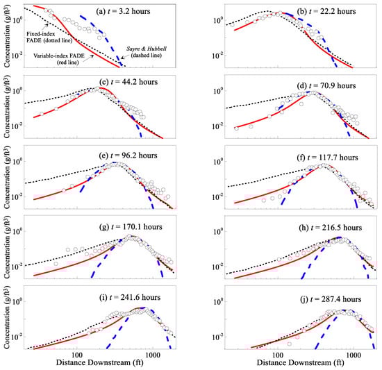
Figure 2.
Application 1: Modeled (red lines, using the variable-index fractional advection-dispersion equation (FADE) (4)) versus measured (circles, by Sayre and Hubbell [47]) snapshots of bed sediment at the North Loup River, Nebraska at ten sampling cycles (a–j). For comparison purposes, the results of the FADE (4) with a fixed index (dotted lines) and the original mode (without considering anomalous diffusion) from Sayre and Hubbell [47] (dashed lines) are also shown.
The model fitting results are shown in Figure 2. The best-fit parameters are: V = 7.75 ft/h (close to the field measurement), (where = 1 [L−1] is used for unit conversion), ftα/h, , and hγ−1.
3.2. Application 2: Heavy Metal Moving in a Stream Varying from Geomorphologic Unit Scale to Watershed Scale
Breakthrough curves (BTCs, representing the time evolution of flux concentration across the control plane) of manganese (Mn) due to mining contamination at the hyporheic flow path scale (0.30 m in length), the reach scale (100~3000 m), and the basin scale (~20,000 m) at Pinal Creek, a perennial river located in the central highlands of Arizona, were measured by Fuller and Harvey [48] (Figure 3a), providing a complete dataset to test the scale effect of anomalous transport. The BTC at the basin scale contains historical data over a period of 15 years (1980~1996) since the Mn concentration began to increase (Figure 3d). The gravel/sand streambed is connected with the underlying alluvial aquifer. Mn moving along the river corridor experiences hydrological and geochemical functions. The TSM (2) captures well the reach-scale BTC, but it misses the nuance of BTCs at the geomorphic unit and watershed scales. A detailed description of heavy metal contamination, the study site, and the application of FADEs can be found in our recent work [1].
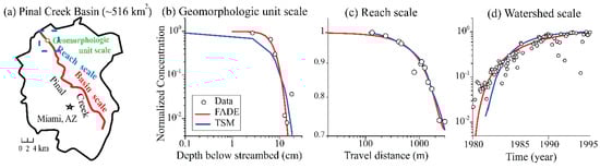
Figure 3.
Application 2: (a) three scales at the Pinal Creek Basin, Arizona (modified from Puckett et al. [1]). (b–d): The measured (symbols) vs. modeled (lines) BTCs using the FADE (7) for the dissolved Mn transport at all three scales in the stream.
Applications show that the following FADE, which is the fundamental fractional advection-dispersion-reaction equation underlying the general expressions (3–5), can fit the observed BTCs at all scales (with the best-fit parameters changing with scales) (see also [1]):
where the reaction term is needed to account for manganese oxidation in the hyporheic zone. Model fitting results are shown in Figure 3 and will be further discussed below.
4. Discussion
4.1. FADE Applicability in Capturing Anoamlous Scaling in Rivers
Application 1 shown in Section 3.1 identified numerically anomalous scaling for bed sediment transport in rivers at local to regional scales, proving the applicability of the single-index FADE (3) at the geomorphologic unit scale and the variable-index FADE (4) at the reach scale. Application 2 in Section 3.2, however, showed that the FADE (7) alone could fit the observed transport for the heavy metal at all three scales. The discrepancy in the model applicability may be due to two reasons. First, bed sediment (which move along the riverbed via saltation, sliding, or rolling and may be affected by the riverbed topography, stream morphology, turbulent boundary layers, shear stress, scour, and entrapment) can be more sensitive to the non-stationary evolution of stream’s hydrologic/geometric properties than the dissolved Mn moving in the open channel. Second, the two applications used different datasets (because different sites used different sampling strategies/tools): Application 1 used the snapshots which covered a full range of the reach, while Application 2 used the BTCs which represent the pollutant flux at a single cross plane. In other words, the trace snapshot provides the instant signal from each sub-region of the riverbed, while the BTC only samples the output signal from the reach (analogous to the output of a black box without information of the detailed, intermediate steps). The BTC calculated by the summation of multiple stochastic processes with different tempered stable densities (i.e., model (4)) may be re-produced by a single stochastic process with the equivalent tempered stable density (i.e., model (7)). Therefore, a variable-index model such as (4) is needed to capture the space-sensitive, non-stationary distribution of snapshots, while the standard FADE with a scale-dependent index can fit the BTCs at the outlet at different scales (according to the generalized central limit theory).
Although the BTC cannot provide detailed spatial information as much as the snapshot, one may still decipher the variation of anomalous transport with scales by analyzing the scale-dependent model parameters when fitting the BTC. This is necessary since in most hydrologic and hydrogeological observations, the BTC is much more common than the snapshot (because the former may require only one sensor). Application 2′s fitting parameters for BTCs do change with scales, which may imply the scaling process. For example, for modeling the Mn BTC at the geomorphologic unit scale at Pinal Creek, the best-fit time index (=) is close to 1 and the best-fit space index is . This might be because at a short travel distance, the Mn particles did not have significant chances to be trapped for a long time before carried/driven by local turbulent flow. At the reach scale, the time index and the space index = 2.00 (fixed at 2) after fitting the BTC; this might be because Mn began to sample more trapping events, and the intermittent turbulence could not cover the whole reach. At the watershed scale, is 1.00 (fixed at 1) and is by fitting the corresponding BTC, because the temporal tempering (i.e., the exponential truncation of the standard α-stable density) produced asymptotic Fickian scaling in time (i.e., sub-diffusion was weakened eventually due to the truncated waiting time PDF), and large floods in the 15 year period generated and accumulated enough fast movement of Mn which cannot be captured by the classical TSM (2), assuming Fickian dispersion. Hence, anomalous transport of Mn in rivers deciphered by fitting the BTCs may be scale dependent, although a single-index model such as the FADE (7) (with a scale-dependent index) can fit all BTCs. This hypothesis, however, requires further validation in the future when abundant field observations are available.
It is also noteworthy that dynamics of anomalous transport may change in time even for the same spatial scale, especially at late times. This was found by our recent work in evaluating the long-term, transient flow dynamics in saturated porous media [49]. At late times, when slow diffusion dominates transient flow, the low-permeability deposits (i.e., clay/silt) began to dominate groundwater head change, whose dynamics can be captured by the fractional-derivative model with a time-variable index similar to the variable-index FADE (4a). The BTCs observed in Application 2 (Figure 3), if they last long enough, may exhibit different scaling behaviors in time because the strong trapping zones would dominate slow diffusion of pollutants at late times. Such a time-scaling behavior may not be identified by a typical snapshot since field monitoring usually cannot last for decades and therefore tends to miss the time-dependent anomalous scaling.
4.2. Fractional Index within a Single Scale: When Will it Reach Stable?
The FADE (7a) (or (3a)) is a macroscopic equation or the scaling limit describing ensemble motion of particles undergoing microscopic random walks with (tempered) power-law jumps and waiting times. The above-mentioned results show that the index of the fractional derivative in the FADEs changes with scales. The hidden assumption is that, for a single scale, the FADE’s index should converge to a stable value. The same assumption was used by almost all FPDEs with a single index, but it has never been checked. Here we check whether this index can reach a stable value by applying the Monte Carlo approach to simulate anomalous transport at various travel distances in a 10-m-long fractured aquifer (Figure 4). The fracture-matrix system (with a length of 10 m), which was generated by COMSOL Multiphysics, contains two smooth, parallel fracture walls with a small, constant aperture of d = 0.0005 m and impermeable matrixes with the width of b = 3 m. A conservative tracer with the concentration of 1 M is injected continuously at the upper boundary for 2 days, and the total modeling time is 10 days. Tracer transport in the fracture is dominated by advection and dispersion longitudinally (i.e., the x axis). The PDE governing the local-scale transport process in the Monte Carlo simulation follows the traditional ADE, with the initial condition and boundary conditions for , for , and . The tracer BTCs (shown by symbols in Figure 5) were collected at 10 locations, representing the travel distance of 0.02, 0.04, 0.08, 0.1, 0.4, 0.8, 1, 4, 8, and 10 m (varying by 3 orders of magnitude), respectively.
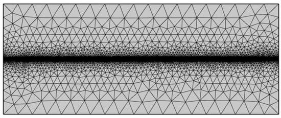
Figure 4.
Finite elements for a laboratory-scale fractured medium, which has a dimension of 10 × 3 m (length × width).
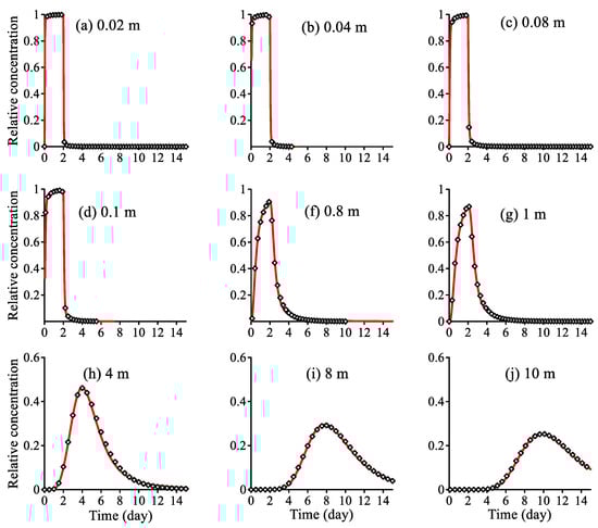
Figure 5.
Fracture: The best-fit (lines, using the FADE (7)) versus the Monte Carlo BTCs (symbols) of dissolved pollutants moving at different travel distances along the saturated fracture-matrix medium plotted in Figure 4.
The single-index FADE (7a) fits all the “measured” BTCs well (Figure 5), with the best-fit parameters listed in Table 2. The resultant mean velocity remains stable due to the steady-state flow condition, and the dispersion coefficient D increases with the travel distance, implying that the tracer particles experience more local fluctuations in velocity when moving further downgradient. The space index since there are no apparent fast jumps along this single fracture. The best-fit time index slowly approaches the asymptote (=0.93) (Table 2 and Figure 6). Before stabilizing at the distance of x ≥ 8 m, the tracer particles move with a relatively constant index within the local scale (x ≤ 1 m). This local scale (1 m) is approximately the hydraulic radius of a single matrix element surrounding the fracture, and hence the tracer particles are moving in a local system with much less variability in the internal structure than those beyond the local scale. Therefore, anomalous transport for pollutants moving inside of a bedform in the riverbed (10−1~100 m), a single hydrofacies in aquifers (10−1~102 m), or the same type of soil in the vadose zone (10−1~101 m) may be captured by the FADE (7) with a stable index. This conclusion explains why the single-index FADE (7a) fits contaminant transport at the well-known MADE aquifer, Mississippi, U.S. (adjacent to fluvial-deltaic deposits of the Gulf of Mexico Basin) and the Cape Cod aquifer, Massachusetts, U.S. (consisting of glacio-fluvial outwash sediments) well [11]. The observed tracer plumes (at the MADE and Cape Cod sites) extended 100~200 m downgradient, which was on the scale of interconnected coarse sand/gravel hydrofacies, and therefore, according to the above-mentioned conclusion, anomalous transport at these two fluvial aquifers can be characterized by the FADE (7a) with a stable index, proving the finding in Zhang et al. [11].
Table 2.
The best-fit parameters in the FADE (7a) for the snapshots shown in Figure 5. In the legend, “RMSE” denotes the root mean square error which evaluates the fitting.
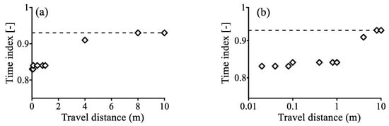
Figure 6.
Fracture: The change of the time index γ in the FADE (7a) with the travel distance for fitting the Breakthrough curves (BTCs) shown in Figure 5. The dashed line shows the asymptote. (b) is the semi-log plot of (a).
Beyond this scale, the fractional index in the FADE tends to apparently fluctuate (Figure 6b), resulting in the variable-index FADE (4) for reach-scale anomalous transport. It is therefore our logic expectation that anomalous transport at the MADE and Cape Cod aquifers would exhibit quite different scaling behaviors when entering the other hydrofacies downgradient. This can cause high uncertainty in predicting the FADE index for anomalous transport in reach-scale rivers or regional-scale aquifers (>200 m), a scale involving many environmental concerns and water resources cleanup efforts. The FADE model predictability at the reach/regional scale remains an open research question. It is also noteworthy that further studies are needed to explore a general theory of stability of the hierarchical FADEs which can be applied to anomalous transport in other complex systems.
5. Conclusions
This study proposed and partially validated the hierarchical fractional-derivative models in simulating anomalous scaling for pollutants transport in the river corridor at all important spatial scales. Three conclusions were drawn. First, the fixed-index FADE (3) captured anomalous transport of bed sediment and the dissolved heavy metal moving in a bedform (i.e., at the geomorphologic unit scale) well, while the variable-index FADE (4) was needed to capture the nuance of bedload snapshots with spatially varying spreading rates along the reach scale riverbed. When the tracer BTC was used, a single index FADE can efficiently upscale anomalous transport without mapping the sub-grid, intermediate, multi-index steps occurring from the source to the reception location, if a scale-dependent index is used in this single-index FADE. Validation of the full capability of the proposed hierarchical FADEs, including the potential temporal scaling of anomalous transport and the distributed-order FADE proposed for capturing watershed-scale snapshots, however, requires further field observations which may be available in the future. Second, pollutant transport in complex geomedia may exhibit anomalous scaling in space, time, or both, and the model selection (including the type and index of the FADE) depends on the scale and type of the geologic system (rivers, aquifers, or soil), as well as the target dataset (snapshot versus BTC). Third, the index of the FADE remains stable at the unit-medium scale, such as the bedform, hydrofacies, and uniform soil, which have different sizes, and then fluctuates beyond this fundamental spatial scale. Therefore, studies of reach-scale anomalous transport (which links the geomorphologic unit scale and the watershed scale) are the core for reliable applications of fractional calculus and FADEs.
Author Contributions
Conceptualization, Y.Z.; methodology, Y.Z. and D.Z.; formal analysis, Y.Z. and D.Z.; investigation, Y.Z.; resources, Y.Z.; data curation, D.Z. and Y.Z.; writing—original draft preparation, Y.Z., D.Z., W.W., J.M.F., H.S., A.Y.S., and X.C.; supervision, Y.Z.; project administration, Y.Z.; funding acquisition, W.W. and H.S. All authors have read and agreed to the published version of the manuscript.
Funding
W.W. was supported partially by the National Natural Science Foundation of China (Grant No. 41931292). D.B.Z. and H.G.S. were funded partially by the National Natural Science Foundation of China (Grant No. 11972148). X.C. was supported by the River Corridor Science Focus Area Project at the Pacific Northwest National Laboratory (PNNL) funded by Department of Energy (DOE), Office of Biological and Environmental Research (BER), as part of BER’s Environmental System Science Program. PNNL is operated for the DOE by Battelle Memorial Institute under contract DE-AC05-76RL01830. Results of this study do not reflect the views of the funding agencies.
Institutional Review Board Statement
Not applicable.
Informed Consent Statement
Not applicable.
Data Availability Statement
Not applicable.
Conflicts of Interest
The authors declare no conflict of interest. The funders had no role in the design of the study; in the collection, analyses, or interpretation of data; in the writing of the manuscript, or in the decision to publish the results.
References
- Puckett, M.H.; Zhang, Y.; Lu, B.Q.; Lu, Y.H.; Sun, H.G.; Zheng, C.M.; Wei, W. Application of fractional differential equation to interpret dynamics of dissolved heavy metal uptake in streams at a wide range of scale. Eur. Phys. J. Plus 2019, 134, 377. [Google Scholar] [CrossRef]
- Boano, F.; Harvey, J.W.; Marion, A.; Packman, A.I.; Revelli, R.; Ridolfi, L.; Wörman, A. Hyporheic flow and transport processes: Mechanisms. models, and biogeochemical implications. Rev. Geophys. 2014, 52, 603–679. [Google Scholar] [CrossRef]
- Winter, T.C. Relation of streams, lakes, and wetlands to groundwater flow systems. Hydrogeol. J. 1999, 7, 28–45. [Google Scholar] [CrossRef]
- Fleckenstein, J.H.; Krause, S.; Hannah, D.M.; Boano, F. Groundwater-surface water interactions: New methods and models to improve understanding of processes and dynamics. Adv. Water Resour. 2010, 33, 1291–1295. [Google Scholar] [CrossRef]
- Brunner, P.; Therrien, R.; Renard, P.; Simmons, C.T.; Franssen, H.J.H. Advances in understanding river-groundwater interactions. Rev. Geophys. 2017, 55. [Google Scholar] [CrossRef]
- Cirpka, O.A.; Valocchi, A.J. Debates-Stochastic subsurface hydrology from theory to practice: Does stochastic subsurface hydrology help solving practical problems of contaminant hydrogeology? Water Resour. Res. 2016, 52, 9218–9227. [Google Scholar] [CrossRef]
- Fiori, A.; Cvetkovic, V.; Dagan, G.; Attinger, S.; Bellin, A.; Dietrich, P. Debates-Stochastic subsurface hydrology from theory to practice: The relevance of stochastic subsurface hydrology to practical problems of contaminant transport and remediation. What is characterization and stochastic theory good for? Water Resour. Res. 2016, 52, 9228–9234. [Google Scholar] [CrossRef]
- Fogg, G.E.; Zhang, Y. Debates—Stochastic subsurface hydrology from theory to practice: A geologic perspective. Water Resour. Res. 2016, 52, 9235–9245. [Google Scholar] [CrossRef]
- Sanchez, V.X.; Fernandez, G.D. Debates –Stochastic subsurface hydrology from theory to practice: Why stochastic modeling has not yet permeated into practitioners? Water Resour. Res. 2016, 52, 9246–9258. [Google Scholar] [CrossRef]
- Metzler, R.; Klafter, J. The random walk’s guide to anomalous diffusion: A fractional dynamics approach. Phys. Rep. 2000, 339, 1–77. [Google Scholar] [CrossRef]
- Zhang, Y.; Meerschaert, M.M.; Baeumer, B.; LaBolle, E.M. Modeling mixed retention and early arrivals in multidimensional heterogeneous media using an explicit Lagrangian scheme. Water Resour. Res. 2015, 51, 6311–6337. [Google Scholar] [CrossRef]
- Baeumer, B.; Kovács, M.; Meerschaert, M.M.; Sankaranarayanan, H. Boundary conditions for fractional diffusion. J. Comput. Appl. Math. 2018, 336, 408–424. [Google Scholar] [CrossRef]
- Baeumer, B.; Kovács, M.; Sankaranarayanan, H. Fractional partial differential equations with boundary conditions. J. Differ. Equ. 2018, 264, 1377–1410. [Google Scholar] [CrossRef]
- Zhang, Y.; Sun, H.G.; Zheng, C.M. Lagrangian solver for vector fractional diffusion in bounded anisotropic aquifers: Development and application. Fract. Calc. Appl. Anal. 2019, 22, 1607–1640. [Google Scholar] [CrossRef]
- Zhang, Y.; Zhou, D.B.; Yin, M.S.; Sun, H.G.; Wei, W.; Li, S.Y.; Zheng, C.M. Nonlocal transport models for capturing solute transport in one-dimensional sand columns: Model review, applicability, limitations and improvement. Hydrol. Process. 2020, 34, 5104–5122. [Google Scholar] [CrossRef]
- Zhang, Y.; Benson, D.A.; Reeves, D.M. Time and space nonlocalities underlying fractional derivative models: Distinction and literature review of applications. Adv. Water Resour. 2009, 32, 561–581. [Google Scholar] [CrossRef]
- Zhang, Y.; Sun, H.G.; Stowell, H.H.; Zayernouri, M.; Hansen, S.E. A review of applications of fractional calculus in Earth system dynamics. Chaos Soliton. Fract. 2017, 102, 29–46. [Google Scholar] [CrossRef]
- Benson, D.A. The Fractional Advection-Dispersion Equation: Development and Application. Ph.D. Thesis, University of Nevada, Reno, NV, USA, 1998. [Google Scholar]
- Horstemeyer, M.F. Multiscale Modeling: A Review. In Practical Aspects of Computational Chemistry; Leszczynski, J., Shukla, M., Eds.; Springer: Dordrecht, The Netherlands, 2009; pp. 87–135. [Google Scholar]
- Andersson, M.; Yuan, J.; Sundén, B. Review on modeling development for multiscale chemical reactions coupled transport phenomena in solid oxide fuel cells. Appl. Energ. 2010, 87, 1461–1476. [Google Scholar] [CrossRef]
- Frayret, C.; Villesuzanne, A.; Pouchard, M.; Matar, S. Density functional theory calculations on microscopic aspects of oxygen diffusion in ceria-based materials. Int. J. Quantum Chem. 2005, 101, 826–839. [Google Scholar] [CrossRef]
- Asproulis, N.; Kalweit, M.; Drikakis, D. Hybrid molecular-continuum methods for micro- and nanoscale liquid flows. In 2nd Micro and Nano Flows Conference; West: London, UK, 2009. [Google Scholar]
- Karttunen, M. Multiscale modelling: Powerful tool or too many promises? In Proceedings of the 2017 SIAM Conference on Computational Science and Engineering, Atlanta, Georgia, 27 February–3 March 2017. [Google Scholar]
- Meerschaert, M.M.; Scheffler, H.P. Limit Theorems for Sums of Independent Random Vectors; John Wiley: New York, NY, USA, 2001. [Google Scholar]
- Visscher, L.; Bolhuis, P.; Bickelhaupt, F.M. Multiscale modelling. Phys. Chem. Chem. Phys. 2011, 13, 10399–10400. [Google Scholar] [CrossRef]
- Famiglietti, J.S.; Wood, E.F. Multiscale modeling of spatially variable water and energy balance processes. Water Resour. Res. 1994, 30, 3061–3078. [Google Scholar] [CrossRef]
- Vannote, R.L.; Minshall, G.W.; Cummins, K.W.; Sedell, J.R.; Cushing, C.E. The river continuum concept. Can. J. Fish. Aquat. Sci. 1980, 37, 130–137. [Google Scholar] [CrossRef]
- Raymond, P.A.; Saiers, J.E.; Sobczak, W.V. Hydrological and biogeochemical controls on watershed dissolved organic matter transport: Pulse-shunt concept. Ecology 2016, 97, 5–16. [Google Scholar] [CrossRef] [PubMed]
- Elliott, A.H.; Brooks, N.H. Transfer of nonsorbing solutes to a streambed with bed forms: Theory. Water Resour. Res. 1997, 33, 123–136. [Google Scholar] [CrossRef]
- Elliott, A.H.; Brooks, N.H. Transfer of nonsorbing solutes to a streambed with bed forms: Laboratory experiments. Water Resour. Res. 1997, 33, 137–151. [Google Scholar] [CrossRef]
- Bencala, K.E.; Walters, R. Simulation of solute transport in a mountain pool-and-riffle stream with a kinetic mass transfer model for sorption. Water Resour. Res. 1983, 19, 718–724. [Google Scholar] [CrossRef]
- Bencala, K.E.; Gooseff, M.N.; Kimball, B.A. Rethinking hyporheic flow and transient storage to advance understanding of streamcatchment connections. Water Resour. Res. 2011, 47, WH00H03. [Google Scholar] [CrossRef]
- Runkel, R.L.; Chapra, S.C. An efficient numerical solution of the transient storage equations for solute transport in small streams. Water Resour. Res. 1993, 29, 211–215. [Google Scholar] [CrossRef]
- Runkel, R.L. One-Dimensional Transport with Equilibrium Chemistry (OTEQ)—A Reactive Transport Model for Streams and Rivers. In Techniques and Methods Book 6, Chap. B6; United States Geological Survey: Reston, Virginia, 2010. [Google Scholar]
- Allison, J.D.; Brown, D.S.; Novo-Gradac, K.J. MINTEQA2/PRODEFA2, A Geochemical Assessment Model for Environmental Systems: Version 3.0 User’s Manual; United States Environmental Protection Agency, Office of Research and Development: Washington, DC, USA, 1991.
- Runkel, R.L.; Kimball, B.A.; McKnight, D.M.; Bencala, K.E. Reactive solute transport in streams: A surface complexation approach for trace metal sorption. Water Resour. Res. 1999, 35, 3829–3840. [Google Scholar] [CrossRef]
- Webster, J.R.; Patten, B.C. Effects of watershed perturbation on stream potassium and calcium dynamics. Ecol. Monogr. 1979, 49, 51–72. [Google Scholar] [CrossRef]
- Harms, T.K.; Cook, C.L.; Wlostowski, A.N.; Gooseff, M.N.; Godsey, S.E. Spiraling down hillslopes: Nutrient uptake from water tracks in a warming arctic. Ecosystems 2019, 22, 1546–1560. [Google Scholar] [CrossRef]
- Cardenas, M.B. Surface water-groundwater interface geomorphology leads to scaling of residence times. Geophys. Res. Lett. 2008, 35, L08402. [Google Scholar] [CrossRef]
- Meerschaert, M.M.; Zhang, Y.; Baeumer, B. Tempered anomalous diffusion in heterogeneous systems. Geophys. Res. Lett. 2008, 35, 1–5. [Google Scholar] [CrossRef]
- Cvetkovic, V. The tempered one-sided stable density: A universal model for hydrological transport? Environ. Res. Lett. 2011, 6, 034008. [Google Scholar] [CrossRef]
- Berkowitz, B.; Cortis, A.; Dentz, M.; Scher, H. Modeling non-Fickian transport on geological formations as a continuous time random walk. Rev. Geophys. 2006, 44, RG2003. [Google Scholar] [CrossRef]
- Baeumer, B.; Haase, M.; Kovacs, M. Unbounded functional calculus for bounded group with applications. J. Evol. Equ. 2009, 9, 171–195. [Google Scholar] [CrossRef]
- Sun, H.G.; Chang, A.L.; Zhang, Y.; Chen, W. A review on variable-order fractional differential equations: Mathematical foundations, physical models, numerical methods and applications. Fract. Calc. Appl. Anal. 2019, 22, 27–59. [Google Scholar] [CrossRef]
- Yin, M.S.; Zhang, Y.; Ma, R.; Tick, G.; Bianchi, M.; Zheng, C.M.; Wei, W.; Wei, S.; Liu, X.T. Super-diffusion affected by hydrofacies mean length and source geometry in alluvial settings. J. Hydrol. 2020, 582, 124515. [Google Scholar] [CrossRef]
- Martin, R.L.; Jerolmack, D.J.; Schumer, R. The physical basis for anomalous diffusion in bed load transport. J. Geophys. Res. 2012, 117, F01018. [Google Scholar] [CrossRef]
- Sayre, W.; Hubbell, D. Transport and Dispersion of Labeled Bed Material; United States Geological Survey Professional Paper 1965; US Government Printing Office: Washington, DC, USA, 1965; Volume 433-C, 48p.
- Fuller, C.C.; Harvey, J.W. Reactive update of trace metals in the hyporheic zone of a mining-contaminated stream, Pinal Creek, Arizona. Environ. Sci. Technol. 2000, 34, 1150–1155. [Google Scholar] [CrossRef]
- Xia, Y.; Zhang, Y.; Green, C.T.; Fogg, G.E. Time-fractional flow equations (t-FFEs) to upscale transient groundwater flow characterized by temporally non-Darcian flow due to medium heterogeneity. 2021. in review. [Google Scholar]
Publisher’s Note: MDPI stays neutral with regard to jurisdictional claims in published maps and institutional affiliations. |
© 2021 by the authors. Licensee MDPI, Basel, Switzerland. This article is an open access article distributed under the terms and conditions of the Creative Commons Attribution (CC BY) license (https://creativecommons.org/licenses/by/4.0/).