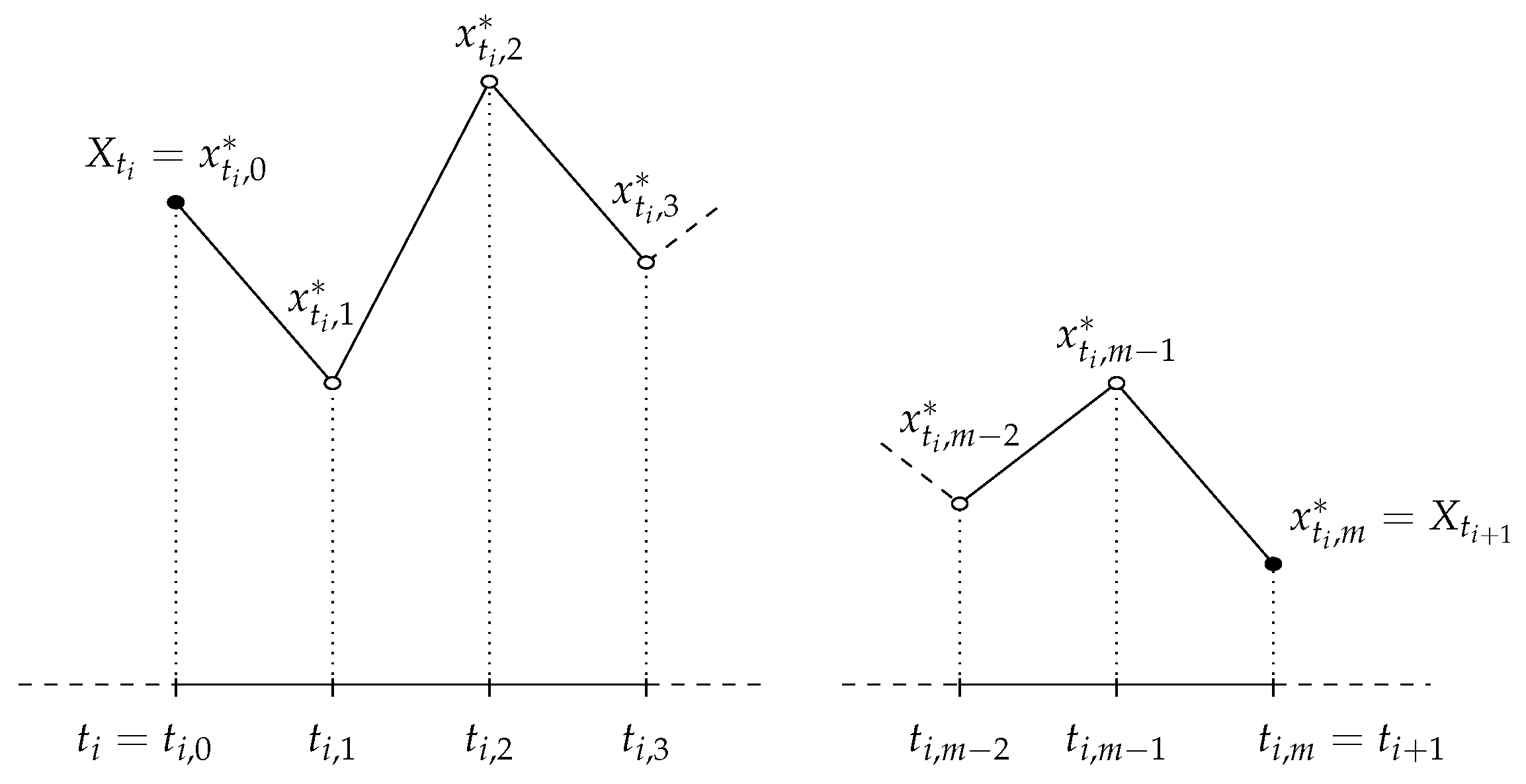
Figure 1.
Augmented data in the discretization scheme: the observed data, and , is augmented by introducing unobserved data points.
Figure 1.
Augmented data in the discretization scheme: the observed data, and , is augmented by introducing unobserved data points.
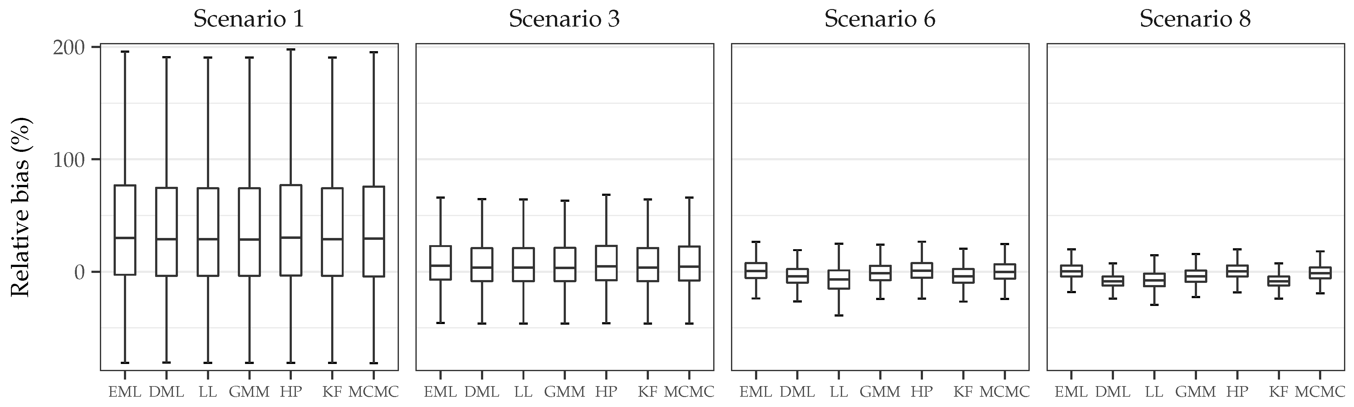
Figure 2.
Relative bias (in percentage) for the drift parameter with weekly data () and .
Figure 2.
Relative bias (in percentage) for the drift parameter with weekly data () and .
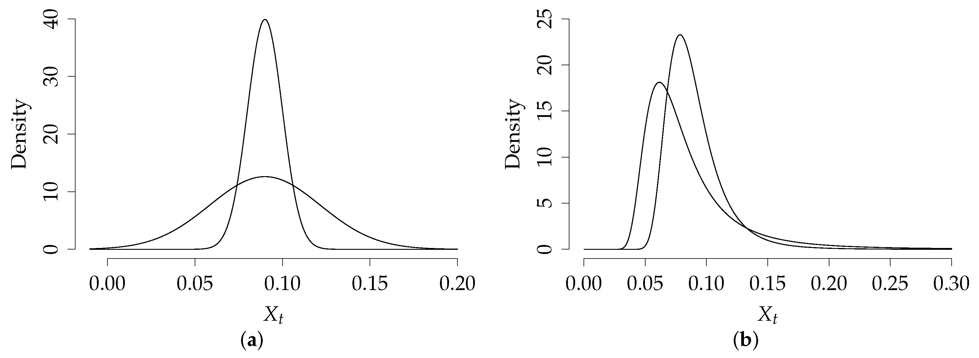
Figure 3.
Vasicek model log-likelihood (ℓ) for the drift parameter with known () and estimated () parameters, where is the true value. The true density and its discretized version () is illustrated, along with the estimate obtained ( and , respectively). Note that scenarios with same but different volatility parameter (scenarios 2, 4, 5 and 7, respectively) are not included, as the estimates were very close and figures very similar to the ones displayed.
Figure 4.
Euribor series. Daily evolution for the time period between 15th October 2001 and 30th December 2005. Sample size for each data set is . From left to right, Euribor 3, 6, 9 and 12 months, respectively.
Figure 4.
Euribor series. Daily evolution for the time period between 15th October 2001 and 30th December 2005. Sample size for each data set is . From left to right, Euribor 3, 6, 9 and 12 months, respectively.
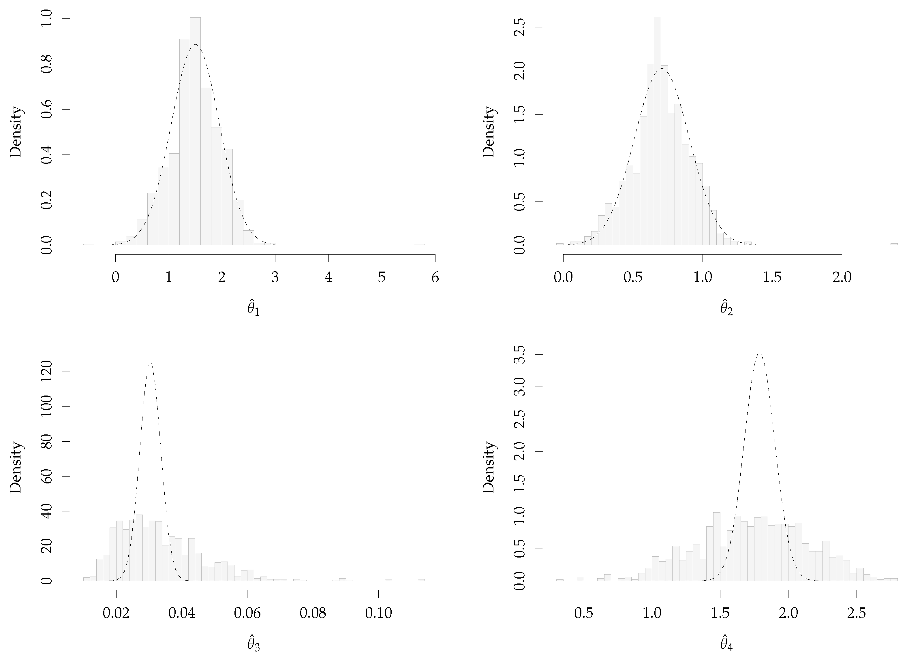
Figure 5.
Bootstrap histogram of , with , and asymptotic Gaussian distribution for the CKLS model, , fitted to Euribor 3 months series.
Figure 5.
Bootstrap histogram of , with , and asymptotic Gaussian distribution for the CKLS model, , fitted to Euribor 3 months series.
Table 1.
Scenarios for the Monte Carlo study for the Vasicek, , and CKLS, , models with .
Table 1.
Scenarios for the Monte Carlo study for the Vasicek, , and CKLS, , models with .
| Vasicek | Scenario 1 | Scenario 2 | Scenario 3 | Scenario 4 |
|---|
| | | | |
| | | | |
| | | | |
| | | | |
| | | | |
| Vasicek | Scenario 5 | Scenario 6 | Scenario 7 | Scenario 8 |
| | | | |
| | | | |
| | | | |
| | | | |
| | | | |
| CKLS | Scenario 1 | Scenario 2 | Scenario 3 | Scenario 4 |
| | | | |
Table 2.
Monte Carlo simulation for Vasicek model, , scenario 1: low mean reversion and low volatility. Boldfaces denote the best results in terms of bias, standard deviation and RMSE.
Table 2.
Monte Carlo simulation for Vasicek model, , scenario 1: low mean reversion and low volatility. Boldfaces denote the best results in terms of bias, standard deviation and RMSE.
| Scenario 1 | , | , | , |
|---|
| Method | | Mean | SD | RMSE | Mean | SD | RMSE | Mean | SD | RMSE |
|---|
| EML | | | | | | | | | | |
| | | | | | | | | |
| | | | | | | | | |
| DML | | | | | | | | | | |
| | | | | | | | | |
| | | | | | | | | |
| LL | | | | | | | | | | |
| | | | | | | | | |
| | | | | | | | | |
| HP | | | | | | | | | | |
| | | | | | | | | |
| | | | | | | | | |
| KF | | | | | | | | | | |
| | | | | | | | | |
| | | | | | | | | |
| MCMC | | | | | | | | | | |
| | | | | | | | | |
| | | | | | | | | |
| GMM | | | | | | | | | | |
| | | | | | | | | |
| | | | | | | | | |
Table 3.
Monte Carlo simulation for Vasicek model, , scenario 3: high mean reversion and low volatility. Boldfaces denote the best results in terms of bias, standard deviation and RMSE.
Table 3.
Monte Carlo simulation for Vasicek model, , scenario 3: high mean reversion and low volatility. Boldfaces denote the best results in terms of bias, standard deviation and RMSE.
| Scenario 3 | , | , | , |
|---|
| Method | | Mean | SD | RMSE | Mean | SD | RMSE | Mean | SD | RMSE |
|---|
| EML | | | | | | | | | | |
| | | | | | | | | |
| | | | | | | | | |
| DML | | | | | | | | | | |
| | | | | | | | | |
| | | | | | | | | |
| LL | | | | | | | | | | |
| | | | | | | | | |
| | | | | | | | | |
| HP | | | | | | | | | | |
| | | | | | | | | |
| | | | | | | | | |
| KF | | | | | | | | | | |
| | | | | | | | | |
| | | | | | | | | |
| MCMC | | | | | | | | | | |
| | | | | | | | | |
| | | | | | | | | |
| GMM | | | | | | | | | | |
| | | | | | | | | |
| | | | | | | | | |
Table 4.
CPU time (in seconds) of the estimation methods per iteration, with .
Table 4.
CPU time (in seconds) of the estimation methods per iteration, with .
| Time (Seconds) | EML | DML | LL | HP | KF | MCMC | GMM |
|---|
| Vasicek | 0.0534 | 0.0469 | 0.0424 | 0.4921 | 0.1097 | 50.8442 | 1.0108 |
| CKLS | - | 0.0818 | 0.2011 | 1.9543 | 0.2017 | 140.5385 | 2.0237 |
| Implementation: | R | R | R | R | C | C++ | R/C++ |
Table 5.
Monte Carlo simulation for CKLS model, , scenario 1: low mean reversion and low volatility. Boldfaces denote the best results in terms of bias, standard deviation and RMSE.
Table 5.
Monte Carlo simulation for CKLS model, , scenario 1: low mean reversion and low volatility. Boldfaces denote the best results in terms of bias, standard deviation and RMSE.
| Scenario 1 | , | , | , |
|---|
| Method | | Mean | SD | RMSE | Mean | SD | RMSE | Mean | SD | RMSE |
|---|
| DML | | | | | | | | | | |
| | | | | | | | | |
| | | | | | | | | |
| | | | | | | | | |
| LL | | | | | | | | | | |
| | | | | | | | | |
| | | | | | | | | |
| | | | | | | | | |
| HP | | | | | | | | | | |
| | | | | | | | | |
| | | | | | | | | |
| | | | | | | | | |
| KF | | | | | | | | | | |
| | | | | | | | | |
| | | | | | | | | |
| | | | | | | | | |
| MCMC | | | | | | | | | | |
| | | | | | | | | |
| | | | | | | | | |
| | | | | | | | | |
| GMM | | | | | | | | | | |
| | | | | | | | | |
| | | | | | | | | |
| | | | | | | | | |
Table 6.
Monte Carlo simulation for CKLS model, , scenario 3: high mean reversion and low volatility. Boldfaces denote the best results in terms of bias, standard deviation and RMSE.
Table 6.
Monte Carlo simulation for CKLS model, , scenario 3: high mean reversion and low volatility. Boldfaces denote the best results in terms of bias, standard deviation and RMSE.
| Scenario 3 | , | , | , |
|---|
| Method | | Mean | SD | RMSE | Mean | SD | RMSE | Mean | SD | RMSE |
|---|
| DML | | | | | | | | | | |
| | | | | | | | | |
| | | | | | | | | |
| | | | | | | | | |
| LL | | | | | | | | | | |
| | | | | | | | | |
| | | | | | | | | |
| | | | | | | | | |
| HP | | | | | | | | | | |
| | | | | | | | | |
| | | | | | | | | |
| | | | | | | | | |
| KF | | | | | | | | | | |
| | | | | | | | | |
| | | | | | | | | |
| | | | | | | | | |
| MCMC | | | | | | | | | | |
| | | | | | | | | |
| | | | | | | | | |
| | | | | | | | | |
| GMM | | | | | | | | | | |
| | | | | | | | | |
| | | | | | | | | |
| | | | | | | | | |
Table 7.
Summary of estimation procedures for SDE parameters.
Table 7.
Summary of estimation procedures for SDE parameters.
| Method | Authors | Asymptotic Properties | Finite Sample Performance |
|---|
| DML | Florens–Zmirou [29] | Asymptotically normal and consistent | Biased when is large |
| LL | Ozaki [17] Shoji and Ozaki [18] | As ML estimators | Outperforms discrete ML and KF |
| HP | Aït–Sahalia [19,47] | Asymptotically normal and consistent [19] | Outperforms LL |
| KF | Kalman [20,48] | Asymptotically normal and consistent [30,34] | Similar to discrete ML |
| MCMC | Elerian et al. [21] Eraker [22] | Simulation based | Efficient but the most computationally intensive |
| GMM | Hansen [23] Chan et al. [6] | Asymptotically normal and consistent [23,41] | The least efficient and efficiency depends on moments |
Table 8.
Estimated parameters and standard errors (in parentheses) for the CKLS model, , fitted to Euribor series using six estimation methods.
Table 8.
Estimated parameters and standard errors (in parentheses) for the CKLS model, , fitted to Euribor series using six estimation methods.
| Method | | 3 Months | 6 Months | 9 Months | 12 Months |
|---|
| DML | | | | | | | | | |
| | | | | | | | |
| | | | | | | | |
| | | | | | | | |
| LL | | | | | | | | | |
| | | | | | | | |
| | | | | | | | |
| | | | | | | | |
| HP | | | | | | | | | |
| | | | | | | | |
| | | | | | | | |
| | | | | | | | |
| KF | | | | | | | | | |
| | | | | | | | |
| | | | | | | | |
| | | | | | | | |
| MCMC | | | | | | | | | |
| | | | | | | | |
| | | | | | | | |
| | | | | | | | |
| GMM | | | | | | | | | |
| | | | | | | | |
| | | | | | | | |
| | | | | | | | |
Table 9.
p-values for the Monsalve-Cobis et al. [
51] goodness-of-fit test for the CKLS parametric form of the drift and diffusion functions.
Table 9.
p-values for the Monsalve-Cobis et al. [
51] goodness-of-fit test for the CKLS parametric form of the drift and diffusion functions.
| Maturity: | 3 Months | 6 Months | 9 Months | 12 Months |
|---|
| p-value drift function | | | | |
| p-value volatility function | <0.001 | <0.001 | | |
Table 10.
Kalman filter estimates, asymptotic standard error and bootstrap standard error of the CKLS model fitted to Euribor 3 months serie.
Table 10.
Kalman filter estimates, asymptotic standard error and bootstrap standard error of the CKLS model fitted to Euribor 3 months serie.
| Parameters: | | | | |
|---|
| Estimation | 1.4964 | 0.7049 | 0.0303 | 1.7899 |
| Asymptotic standard error | 0.4492 | 0.1964 | 0.0031 | 0.1121 |
| Bootstrap standard error | 0.4794 | 0.2105 | 0.0653 | 0.4110 |


