An Approximation of Solutions for the Problem with Quasistatic Contact in the Case of Dry Friction

Abstract

In this paper, we discuss the question of finding an optimal control for the solutions of the problem with dry friction quasistatic contact, in the case that the friction law is modeled by a nonlocal version of Coulomb’s law. In order to get the necessary optimality conditions, we use some regularization techniques, and this leads us to a problem of control for an inequality of the variational type. The optimal control problem consists, in our case, of minimizing a sequence of optimal control problems, where the control variable is given by a Neumann-type boundary condition. The state system is represented by a limit of a sequence, whose terms are obtained from the discretization, in time with finite difference and space with the finite element method of a regularized quasistatic contact problem with Coulomb friction. The purpose of this optimal control problem is that the traction force (the control variable) acting on one side of the boundary (the Neumann boundary condition) of the elastic body produces a displacement field (the state system solution) close enough to the imposed displacement field, and the traction force from the boundary remains small enough.

1. Introduction

The quasistatic model of the contact problems implies ignoring the inertial effects. In addition, we specify that the modeling of the boundary conditions must be given by time-dependent functions. We assume that the hypotheses imposed by the theorems of existence and uniqueness are fulfilled, including conditions of regularity and a small enough friction coefficient [1,2]. Because of the great computational effort, a better choice of the quasistatic formulation is to be used, instead of the dynamic formulation of the contact problem; some similar useful results can be found in [3,4,5]. Using temporal discretization, we obtain an incremental issue that is equivalent to a sequence of static contact problems, and the sequence of solutions of these static contact problems converges to the solution of the quasistatic problem. Another important feature of the quasistatic model is that it allows the size of the contact area, generally unknown, to be approximated much better than with other methods, and this is because after each incremental step, it is possible to check the actual size of the contact area. It is obtained by checking the contact status, in each time interval, of the nodes describing the presumed contact area. Of the main results in this field, we recall one as [6,7,8,9]. The study of an optimal numerical control problem involves the following steps: the existence of a solution; optimal conditions; the numerical approximation of the problem and the numerical solving of the discrete control problem. We intend to approach only the first three steps. In order to fulfill the necessary conditions of optimality, in the control problem of a variational inequality with a non-differential term, we use some regularity techniques. The authors of the article aim to: provide a correct (well-posed) formulation of quasistatic contact problems with friction in elasticity, present the necessary and sufficient hypotheses for the existence and uniqueness of the solution, perform the discretization in space and time of equilibrium equations, and use regularization methods to avoid non-differentiable terms and convergent and numerically stable minimization algorithms for solving boundary optimal control problems. The novelty of the article is solving the problem of optimal control on the contact boundary, since the regularized problem of quasistatic contact with friction in elasticity fulfills the necessary conditions. This problem is of great importance in engineering applications (for example, for mobile robots and manipulator robots), where the control of forces and the control of displacements, as well as the control of sliding contact and/or fixed contact play a major role. The outline of the article is as follows. The equilibrium equations of the quasistatic frictional contact problem in classical and variational form are described in Section 2. Section 3 contains the discretization, in time (with finite difference) and space (with the finite element method), of the quasistatic problem with friction, and in Section 4, we describe the problem of boundary optimal control. Section 5 presents the problem of regularized boundary optimal control.

2. Presentation of Equilibrium Equations in Classical and Variational Form

We consider $\mathrm{\Omega }\subset R^d$ (where d can be three or two), a region that is filled by an elastic material having a Lipschitzian border denoted by $\mathrm{\partial }\mathrm{\Omega }$. Consider $\mathrm{\partial }{\mathrm{\Omega }}_C$, $\mathrm{\partial }{\mathrm{\Omega }}_1$, and $\mathrm{\partial }{\mathrm{\Omega }}_2$ three subsets of $\mathrm{\partial }\mathrm{\Omega }$, which are assumed to be disjointed such that:

$$\mathrm{\partial }\mathrm{\Omega }={\overline{\mathrm{\partial }\mathrm{\Omega }}}_1\cup {\overline{\mathrm{\partial }\mathrm{\Omega }}}_2\cup {\overline{\mathrm{\partial }\mathrm{\Omega }}}_C,$$

$${\overline{\mathrm{\partial }\mathrm{\Omega }}}_1\cap {\overline{\mathrm{\partial }\mathrm{\Omega }}}_C=⌀$$

and mes$(\mathrm{\partial }{\mathrm{\Omega }}_1)>0$. On the elastic body $\mathrm{\Omega }$, the following forces act: the density volume force $\mathit{f}\in \mathrm{\Omega }\times [0,T]$; the traction force $\mathit{h}$ acting on $\mathrm{\partial }{\mathrm{\Omega }}_2\times [0,T]$; and on the $\mathrm{\partial }{\mathrm{\Omega }}_1$ side of the boundary, the body $\mathrm{\Omega }$ is embedded on a rigid foundation. On the ${\mathrm{\partial }\mathrm{\Omega }}_C$ side of the boundary, the Coulomb friction law acts, and it is necessary to satisfy the unilateral contact conditions.

Let $\mathit{u}(\mathit{x},\mathit{t})=(u_1(x,t),\dots ,u_d(x,t))$ be the vector field of displacement,

$$\mathbf{\epsilon }=\left({\epsilon }_{ij}\left(\mathbf{u}\right)\right)=\left(\frac{1}{2}(u_{j,i}+u_{i,j})\right)$$

the tensor field of strain, and:

$$\mathbf{\tau }=\left({\tau }_{ij}\left(\mathbf{u}\right)\right)=\left({\overline{a}}_{ijmn}{\epsilon }_{mn}\left(\mathbf{u}\right)\right)$$

the tensor field of stress, where $i,j,m,n=1,\dots ,d$. Denote by ${\mathbf{u}}_N=u_i·n_i$, the normal components of the displacement vector, by ${\mathit{u}}_T=\mathit{u}-{\mathit{u}}_N·\mathbf{n}$, the tangential components of the displacement vector, and with ${\mathbf{\tau }}_N={\mathbf{\tau }}_{ij}{u}_i{n}_j$, the normal components of the stress vector, where ${\left({\mathbf{\tau }}_T\right)}_i={\mathbf{\tau }}_{ij}{n}_j-{\mathbf{\tau }}_N·n_i$, tangential components of the stress vector, and by $\mathbf{n}=\left(n_i\right)$ the components of the unit normal, which is outward $\mathrm{\partial }\mathrm{\Omega }$.

Let us denote by $g\ge 0$, $g\in C\left({\overline{\mathrm{\partial }\mathrm{\Omega }}}_C\right)$, the initial interstice that appears between the domain $\mathrm{\Omega }$ and the foundation, which is rigid, and it is measured along the outward normal direction on $\mathrm{\partial }{\mathrm{\Omega }}_C$. We assume that the material constants in Hooke’s law ${\overline{a}}_{ijmn}\in L^{\infty }\left(\mathrm{\Omega }\right)$, $l\le i,j,m,n\le d$, fulfill the following conditions:

$${\overline{a}}_{ijmn}={\overline{a}}_{jimn}={\overline{a}}_{mnij},1\le i,j,m,n\le d,$$

$$\mathrm{and}\exists m_1>0,\forall \varphi =\left({\varphi }_{ij}\right)\in R^{d^2},{\varphi }_{ij}={\varphi }_{ji},1\le i,j\le d,$$

$${\overline{a}}_{ijmn}{\varphi }_{ij}{\varphi }_{mn}\ge m_1{\left|\varphi \right|}^2.$$

It follows that the tensor $\left({\overline{a}}_{ijmn}\right)$ is invertible, and we denote by $\left({\overline{b}}_{ijmn}\right)$ its inverse, resulting in that it can be written as:

$${\epsilon }_{ij}\left(\mathit{v}\right))={\overline{b}}_{ijmn}{\tau }_{mn}\left(\mathit{v}\right),$$

for $i,j,m,n=1,\dots ,d$.

The classical form of the quasistatic problem of contact with friction, where the normal stress ${\tau }_N\left(v\right)$ and $\mathrm{\partial }{\mathrm{\Omega }}_C$ are considered known, is:

Find $\mathit{u}=\mathit{u}\left(x,t\right)$ with the initial condition $\mathit{u}(0,·)={\mathit{u}}^0(·)$, in $\mathrm{\Omega }\times [0,T]$ and for all $t\in [0,T]$, s.t.:

$$-\mathrm{div}\mathbf{\tau }\left(\mathit{u}\right(\mathit{x},\mathit{t}\left)\right)=\mathit{f}(\mathit{x},\mathit{t}),\mathrm{in}\mathrm{\Omega }\times [0,T],$$

(1)

$${\mathbf{\tau }}_{ij}\left(\mathit{u}(\mathit{x},\mathit{t})\right)=a_{ijmn}·{\mathbf{\epsilon }}_{mn}\left(\mathit{u}(\mathit{x},\mathit{t})\right),\mathrm{in}\mathrm{\Omega }\times [0,T],$$

(2)

$$\mathit{u}(\mathit{x},\mathit{t})=0\mathrm{on}\mathrm{\partial }{\mathrm{\Omega }}_1\times [0,T],$$

(3)

$$\mathbf{\tau }(\mathit{x},\mathit{t})·\mathit{n}=\mathit{h}(\mathit{x},\mathit{t})\mathrm{on}\mathrm{\partial }{\mathrm{\Omega }}_2\times [0,T],$$

(4)

the contact condition:

$$\begin{array}{cc}\hfill u_N(x,t)\le g(x,t),& {\mathbf{\tau }}_N\left(u(x,t)\right)\le 0,\hfill \\ \hfill & (u_N(x,t)-g(x,t)){\mathbf{\tau }}_N\left(u(x,t)\right)=0,\forall (x,t)\in \mathrm{\partial }{\mathrm{\Omega }}_C\times [0,T],\hfill \end{array}$$

(5)

and Coulomb’s law of friction on $\mathrm{\partial }{\mathrm{\Omega }}_C$:

$$\begin{array}{cc}\hfill \parallel {\tau }_T\left(v\right)\parallel & \le {\mu }_F\left|{\tau }_N\left(v\right)\right|,\mathrm{a}.\mathrm{e}.:\hfill \\ \hfill & -\mathrm{if}\parallel {\tau }_T\left(v\right)\parallel <{\mu }_F\left|{\tau }_N\left(v\right)\right|\Rightarrow v_T=0,\hfill \\ \hfill & -\mathrm{if}\parallel {\tau }_T\left(v\right)\parallel ={\mu }_F\left|{\tau }_N\left(v\right)\right|\Rightarrow \exists \lambda \ge 0,\mathrm{such}\mathrm{that}{\dot{v}}_T=-\lambda {\tau }_T,\hfill \end{array}$$

(6)

in which the coefficient of friction according to Coulomb’s law is considered known: ${\mu }_F\in L^{\infty }(\mathrm{\partial }{\mathrm{\Omega }}_C)$, where ${\mu }_F\ge {\mu }_0$, almost everywhere on $\mathrm{\partial }{\mathrm{\Omega }}_C$.

For the variational form, it is necessary to introduce the following notions: the space of admissible displacements:

$$V=\left\{v\in {\left(H^1\left(\mathrm{\Omega }\right)\right)}^2|v=0\mathrm{on}\mathrm{\partial }{\mathrm{\Omega }}_1\right\}$$

and we will also note the convex subset of kinematically admissible displacements:

$$K=\{v_N\in V|v_N\equiv v·n\le g\mathrm{on}\mathrm{\partial }{\mathrm{\Omega }}_C\}.$$

To model the Coulomb friction law, (6), and the contact conditions, (5), we proceed as follows:

-

We assume that it is possible to determine that the non-negative slip constrained $s_T\in L^{\infty }(\mathrm{\partial }{\mathrm{\Omega }}_C)$ is equal to the product between the friction coefficient ${\mu }_F$ and normal stress ${\lambda }_1$, considered known, i.e., $s_T={\mu }_F{\lambda }_1$;

-

The normal reaction at the contact interface is approximated with the law of normal compliance:

$${\tau }_N\left(u\right)=-c_N{(u_N-g)}_{+}^{m_N}$$

in which the constants $c_N$ and $m_N$ are material parameters revolving around the interface properties; notation ${(.)}_{+}$ means: ${\left(b\right)}_{+}$= max $(b,0)$; ${\dot{u}}_T$ is tangential velocity on $\mathrm{\partial }{\mathrm{\Omega }}_C$.

With these specifications, the variational formulation of the quasistatic contact problem with friction (see [10,11]) becomes:

Problem 1

($P_1$). Let us find the function $u(x,t)\in K\times [0,T]$ so that:

$$\tilde{a}(u\left(t\right),v-\dot{u}\left(t\right))+j_1(u\left(t\right),v-\dot{u}\left(t\right))\ge {(L\left(t\right),v-\dot{u}\left(t\right))}_V\forall v\in V,$$

for any $t\in [0,T],T>0$, which satisfies the initial condition $u(x,0)=u_0$, where:

$$\tilde{a}(w,u)={\int }_{\mathrm{\Omega }}{a}_{ijkl}{\epsilon }_{ij}\left(w\right){\epsilon }_{kl}\left(u\right)dx\forall w,u\in V,$$

$${(L\left(t\right),v)}_V={\int }_{\mathrm{\Omega }}f\left(t\right)vdx+{\int }_{\mathrm{\partial }{\mathrm{\Omega }}_2}h\left(t\right)vds\forall v\in V,$$

$$j_1(u,v)={\int }_{\mathrm{\partial }{\mathrm{\Omega }}_C}{s}_T\left|v_T\right|ds+{\int }_{\mathrm{\partial }{\mathrm{\Omega }}_C}{c}_N{(u-g)}^{m_n}{v}_{N}ds\forall u,v\in V.$$

Additionally, $v_T\in {\left(L^{\infty }(\mathrm{\partial }{\mathrm{\Omega }}_C)\right)}^{d-1}$ is the tangent vector to boundary $\mathrm{\partial }{\mathrm{\Omega }}_C$. We also assume that the initial condition satisfies the compatibility requirement:

$$\overline{a}(u_0,v)+j_1(u_0,v)\ge {(L\left(0\right),v)}_V,\forall v\in V.$$

Problem 1 ($P_1$) is considered non-differentiable, as a result of the previously defined term $j_1$ (more precisely because of the module function). Under the hypothesis that ${\mu }_F$ is adequately small and $mes(\mathrm{\partial }{\mathrm{\Omega }}_0)>0$, according to [9,12], the quasi-variational inequality, mentioned above, has a unique solution.

3. A Discretization of the Problems of Contact with Coulomb-Type Friction

In this section, we present the algorithm for the time discretization of the quasistatic contact problem, Problem 1 ($P_1$).

Considering a division of the interval $[0,T]$ by the points $(t^0,t^1,\dots ,t^N)$, it results in a new formulation of Problem (P${}_1$), one of an incremental type, in which we use an approximation for the derivative of the function u with respect to time, with the help of the backward finite difference.

Considering:

$$u^k=u(x,t^k),\Delta u^k=u^{k+1}-u^k,$$

$$\Delta t^k=t^{k+1}-t^k,$$

$$\dot{u}\left(t^{k+1}\right)=\Delta u^k/\Delta t,$$

$$L^k=L^{k+1}-L^k,fork=0,1,\dots ,N-1$$

where:

$$\Delta t=\frac{T}{N},$$

we attain, for any time $t^k$, the succeeding discreet quasi-variational inequality:

Problem 2

($P_1^t$). Find $\Delta u^k\in V$ so that:

$$\begin{array}{c}\hfill \overline{a}(\Delta u^k,v-\Delta u^k/\Delta t^k)+j_1(\Delta u^k,v-\Delta u^k/\Delta t^k)\ge \\ \hfill \ge \Delta L^k(v-\Delta u^k/\Delta t^k)-F(u^k,v-\Delta u^k/\Delta t^k),\forall v\in K_h,\end{array}$$

where:

$$\begin{array}{c}\hfill F(u^k,v-\Delta u^k/\Delta t^k)=\\ \hfill =\overline{a}(u^k,v-\Delta u^k/\Delta t^k)-L^k(v-\Delta u^k/\Delta t^k),\forall 0\le k\le n-1.\end{array}$$

For spatial discretization with the finite element method (see [13]), we consider a family of finite element subspaces generated by a basis of a piecewise linear function, which correspond to a regular family of partitions of body $\mathrm{\Omega }$, compatible with the boundary decomposition of:

$$\mathrm{\partial }\mathrm{\Omega }=\mathrm{\partial }{\mathrm{\Omega }}_1\cup \mathrm{\partial }{\mathrm{\Omega }}_2\cup \mathrm{\partial }{\mathrm{\Omega }}_C.$$

With the two discretizations, in time and space, obtained, one can write a form similar to the temporal discretization where one is looking for $\Delta u_h^k\in V_h$, for each $t^k\in [0,T]$. We use a much more numerically appropriate formulation, namely one obtained with the use of a sequential quadratic programming technique:

Problem 3

($P_1^{ht}$). Find $\mathbf{u}\in {\mathbf{K}}_{\mathbf{h}},\mathrm{for}\mathrm{each}\mathrm{time}$$t^k\in [0,T]$ so that:

$${\mathbf{J}}_{\mathbf{h}}\left(\mathbf{u}\right)=\underset{\mathbf{v}\in {\mathbf{K}}_{\mathbf{h}}}{min}{\mathbf{J}}_{\mathbf{h}}\left(\mathbf{v}\right),$$

where

$$\begin{array}{c}\hfill \mathbf{u}\equiv \Delta u_h^k,\mathbf{v}\equiv v_h,\\ \hfill {\mathbf{J}}_{\mathbf{h}}\left(\mathit{v}\right)=\frac{1}{2}{\mathit{v}}^T{\mathit{K}}_{\mathbf{n}}\mathit{v}-{\mathit{v}}^T{\mathit{f}}_{\mathbf{n}}+{\mathit{p}}_{\mathbf{m}}^T\left|\mathit{Tv}\right|,\end{array}$$

and:

$$K_h=\left\{\mathit{v}{\in }^n\right|\mathit{Nv}\le \mathit{g}\}.$$

We consider ${\mathit{K}}_{\mathbf{n}}\in R^{n\times n}$ to be the stiffness matrix. ${\mathit{f}}_{\mathbf{n}}\in R^n$ is the load force vector, and ${\mathit{p}}_{\mathbf{m}}\in R^m$ is a constrained vector for the nodal slip for the nodes of contact. The matrices $\mathit{N},\mathit{T}\in R^{m\times n}$ represent the rows of the tangential and normal vectors corresponding to the nodes of contact, respectively, and $\mathit{g}\in R^m$ is the vector defined by distances between the the solid foundation and nodes of contact.

The main characteristic features of the approximation of the problem of elastic frictional contact using the finite element method are the following. In the two-dimensional case, the finite contact element has three nodes, and in the three-dimensional case, it has four nodes. The third node, respectively the fourth node, aims to detect the interstice (space) in the respective contact area, which can change during loading.

Figure 1 and Figure 2 show the finite contact elements.

In this way, for each change in load force corresponding to the time interval, the contact can be treated as open, closed, or sliding (stick-slip). In addition, the finite contact element will require compliance with the contact condition by penalizing non-compliance.

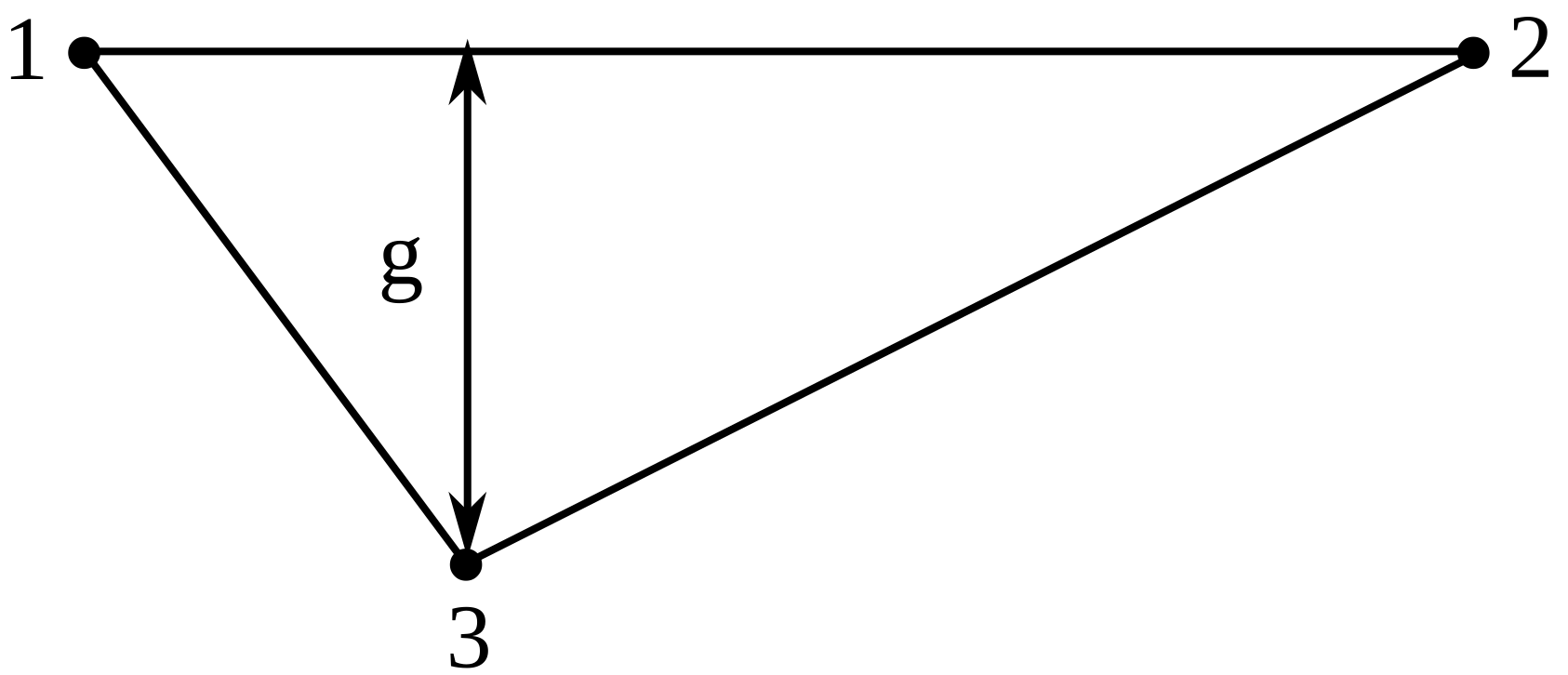
In Figure 3, the chosen example is presented, which has the advantage that it is simple and the contact area contains all three states (fixed-stick, sliding, and open). In addition, due to the symmetry, we modeled only half, the part drawn with a continuous line. The contact area between the flat plate and the foundation was modeled with the finite contact element with three nodes, and the area in its vicinity was more finely discretized in order to better approximate the three types of contact states. In

Table 1. The results for different loads and different coefficients of friction for the example presented.

$\mathit{\mu }$	F	f	Open Contact	Sliding Contact	Stick Contact
	daN/	daN/	Zone $\mathit{AB}$	Zone $\mathit{BC}$	Zone $\mathit{CD}$
	mm${}^2$	mm${}^2$	mm	mm	mm
1	10	−5	3.75	20	16.25
1	15	−5	5	20.75	7.5
0.2	10	−5	0	40	0
0.2	10	−15	0	22.5	17.5
0.2	10	−25	0	5	35

, we present the results for different loads and different coefficients of friction (the case $\mu$ = 1 is only of theoretical interest). For each of the five calculated variants, we proceed as follows: at each load increment, the program performs a number of iterations until the error condition is satisfied (the difference between two consecutive iterations should be small enough). The incremental loading method approximates the loading history well and implicitly those three types of contact areas, and the iterative algorithm models the Newton-Raphson method used in the approximation of nonlinearities. By means of the third node in the 2D case, respectively the fourth node in the 3D case, the gap between the contact areas is determined and implicitly the type of contact node (fixed-stick, sliding, or open), and the friction law is introduced in the case of sliding contact and makes the application of the penalty method that prevents the interpenetration of the two bodies in contact possible. This third, respectively the fourth, node belongs to the foundation, respectively to the contact boundary of the one of the second elastic body in contact with the first, in the case of two elastic bodies in contact.

4. A General Formulation for the Problem of Boundary Optimal Control

Boundary optimal control of Problem 1 ($P_1$) consists of finding a control variable, represented by the traction force acting on the boundary $\mathrm{\partial }{\mathrm{\Omega }}_2$ of the elastic body. The solution (the displacement field) of the state system requires being an approximation as good as possible for the sought result (the vector field of displacement), as well as the traction force being small enough and minimizing a cost function.

For solving the boundary optimal control problem, we begin with defining the state problem:

Problem 4

($S{P}_1$). Assume that $\mathit{h}\in L^2{(\mathrm{\partial }{\mathrm{\Omega }}_2)}^{d-1}$, which is called optimal control, is a given function. Let us determine the function $\mathit{u}\in V$, which satisfies the following inequality:

$$\tilde{a}(v,w-v)+j_1(v,w)-j_1(v,v)\ge (L,v-w)\forall \mathit{w}\in V.$$

In light of Problem 1 ($P_1$), for any given value for the function $\mathit{h}\in L^2{(\mathrm{\partial }{\mathrm{\Omega }}_2)}^{d-1}$, the above Problem 4 ($S{P}_1$) admits a singular acceptable solution for any $\mathit{v}\in V$, where $\mathit{v}=\mathit{v}\left(\mathit{h}\right)$.

Now, we introduce the next functional:

$$\overline{J}:L^2{(\mathrm{\partial }{\mathrm{\Omega }}_2)}^{d-1}\times V\to R,$$

defined by:

$$\begin{array}{c}\hfill \overline{J}(\mathit{h},\mathit{v})=\frac{1}{2}\parallel \mathit{v}-{\mathit{v}}_{\mathit{d}}{\parallel }_V+\frac{\alpha }{2}{\parallel \mathit{h}\parallel }_{L^2{(\mathrm{\partial }{\mathrm{\Omega }}_2)}^{d-1}}\end{array}$$

(7)

where $\alpha$ is a positive constant and ${\mathit{v}}_{\mathit{d}}$ is the goal function (the desired deformation). We designate:

$$V_{ad}=\left\{[\mathit{h},\mathit{v}]|[\mathit{h},\mathit{v}]\in L^2{(\mathrm{\partial }{\mathrm{\Omega }}_2)}^{d-1}\times V,s.t.\left(\mathit{SP}\mathbf{1}\right)issatisfied\right\},$$

Considering that our aim is to study a control present on the boundary $\mathrm{\partial }{\mathrm{\Omega }}_2$, this determines that the sought-after stress tensor $\mathbf{\tau }$ be as viable as possible for the imposed target:

$${\mathbf{\tau }}_{\mathit{d}}=\left({\tau }_{ij}\left({\mathbf{v}}_{\mathbf{d}}\right)\right)=\left({\overline{a}}_{ijkl}{\epsilon }_{kl}\left({\mathbf{v}}_{\mathbf{d}}\right)\right).$$

Let Problem (OC1) be the following problem of optimal control:

Problem 5

($O{C}_1$). Determine $[\overline{\mathit{h}},\overline{\mathit{v}}]\in V_{ad}$ such that:

$$\overline{J}(\overline{\mathit{h}},\overline{\mathit{v}})=\underset{[\mathit{h},\mathit{v}]\in V_{ad}}{min}\overline{J}(\mathit{h},\mathit{v});$$

thus, the solution of the problem $\left({\mathit{OC}}_{\mathbf{1}}\right)$ is named an optimal pair, and the second part of this pair is called an optimal control.

With the above results, the following theorem can be enunciated:

Theorem 1.

Problem 5 has at worst one solution $[\overline{\mathit{h}},\overline{\mathit{u}}]$.

5. The Optimal Control Problem for the Regularized Contact State

To attain the optimal control algorithm, we begin by regularizing the non-differentiable friction functional $j_1$. For this purpose, the functional $j_1$ is approximated by using a convex and differentiable family of functionals $j_r$, with respect to the second variable.

$$j_r:V\times V\to R,j_r(v,w)=\underset{\mathrm{\partial }{\mathrm{\Omega }}_C}{\int }{s}_T{\psi }_r\left(w_T\right)ds+{\int }_{\mathrm{\partial }{\mathrm{\Omega }}_C}{c}_N{(v-g)}^{m_n}{w}_{N}ds$$

where we denote by:

$${\psi }_r:{\left(L^2(\mathrm{\partial }{\mathrm{\Omega }}_C)\right)}^{d-1}\to L^2(\mathrm{\partial }{\mathrm{\Omega }}_C)$$

an approximation for the function modulus:

$$|·|:{\left(L^2(\mathrm{\partial }{\mathrm{\Omega }}_C)\right)}^{d-1}\to L^2(\mathrm{\partial }{\mathrm{\Omega }}_C).$$

This can be exemplified in numerous ways, i.e., for $r>0$, $\xi \in {\left(L^2(\mathrm{\partial }{\mathrm{\Omega }}_C)\right)}^{d-1}$ and $x\in \mathrm{\partial }{\mathrm{\Omega }}_C$:

$${\psi }_r\left(\xi \right)=\left\{\begin{array}{cc}r|\frac{\xi }{r}{|}^2\left(1-\frac{1}{3}\left|\frac{\xi }{r}\right|\right),\hfill & \mathrm{if}\left|\xi \right(x\left)\right|\le r\hfill \\ \left(\left|\frac{\xi }{r}\right|-\frac{1}{3}\right),\hfill & \mathrm{if}\left|\xi \right(x\left)\right|>r.\hfill \end{array}\right.$$

The most frequent example for a regularization function is:

$${\psi }_r\left(\xi \right)=\sqrt{{\parallel \xi \parallel }^2+r},or{\psi }_r\left(\xi \right)=\sqrt{{\parallel \xi \parallel }^2+r^2}-r.$$

In this instance, we substitute the state Problem 4 ($S{P}_1$) with the succeeding regularized state problem:

Problem 6

($RS{P}_1$). Assume that $\mathit{h}\in L^2{(\mathrm{\partial }{\mathrm{\Omega }}_2)}^{d-1}$ is a known function, and it is called regularized control.

Let us determine the function $v\in V$, s.t.:

$$\tilde{a}(v,w-v)+j_r(v,w)-j_r(v,)\ge (L,v-w)\forall w\in V.$$

The state problem of regularization Problem 6 ($RS{P}_1$) has one solution ${\mathit{u}}_{\mathit{r}}\in V$, which is continuously contingent on the functional L, which is linear; see [14].

In these hypotheses, for any $\mathit{h}\in L^2{(\mathrm{\partial }{\mathrm{\Omega }}_2)}^{d-1}$, the above Problem 6 ($RS{P}_1$) admits only one solution $\forall \mathit{w}\in V,\mathit{v}=\mathit{v}\left(\mathit{h}\right)$.

Considering the following set:

$$V_{ad}^r=\left\{[\mathit{h},\mathit{v}]|[\mathit{h},\mathit{v}]\in L^2{(\mathrm{\partial }{\mathrm{\Omega }}_2)}^{d-1}\times V,s.t.\left(RSP1\right)issatisfied\right\},$$

we have all the necessary data for successfully defining the regularized optimal $\mathrm{Problem} 7 \left(ROC\right)$:

Problem 7

($ROC$). Find $[{\mathit{h}}^{\ast },{\mathit{u}}^{\ast }]\in V_{ad}^r$ such that:

$$J_r({\mathit{h}}^{\ast },{\mathit{v}}^{\ast })=\underset{[\mathit{h},\mathit{v}]\in V_{ad}^r}{min}{J}_r(\mathit{h},\mathit{v}).$$

Thus, we can define the next theorem:

Theorem 2.

The above $\mathrm{Problem} 7 \left(ROC\right)$ admits at worst one solution $[{\mathit{h}}^{\ast },{\mathit{v}}^{\ast }]$.

A solution of the above $\mathrm{Problem} 7 \left(ROC\right)$ is named an optimal pair of regularization. The second element of this pair is called a regularized optimal control.

This is an infinite optimal control problem where we use variational methods, and to avoid the term non-differentiable in the equilibrium equation, we use regularization methods. The finite element method for spatial discretization and finite differences for temporal discretization lead to a finite optimal control problem.

It is known that the finite-dimensional optimal control problem has a solution. The generalized penalty method can be used to transform the restriction optimization problem into a sequence of unrestricted optimization problems (see [15]). The generalized penalty method uses two important properties (methods): the so-called barrier methods (uses the barrier logarithmic functions) and the penalty methods for which the penalty is designed as a regularization of the handling of multiplier values. Problems without restrictions are built with an additional term for the cost function, which consists of a penalty parameter that is a measure of the violation of restrictions. The sequence of the solutions of the problems without restrictions converges to the optimal result.

In order to justify the theorem of the existence of a boundary optimal control problem, we analyze the following boundary value problem with Neumann boundary conditions, with the following specifications: the domain is the square unit $\mathrm{\Omega }=[0,1]\times [0,1]$, the cost functional that is to be minimized and with inequality constraints on the control and states. The boundary of the domain is: $\begin{array}{c}\hfill \mathrm{\partial }\mathrm{\Omega }\equiv \Gamma =\left\{\right(x,0)\cup (x,1\left)\right|0\le x\le 1\}\cup \{(0,y)\cup (1,y)|0\le y\le 1\}.\end{array}$

Consider the partial differential equation with Neumann boundary conditions: $\begin{array}{l}-\Delta w(x,y)-exp\left(w\right(x,y\left)\right)=u(x,y)on\mathrm{\Omega }\\ \frac{\mathrm{\partial }w(x,y)}{\mathrm{\partial }n}+w(x,y)=0on\Gamma ,\end{array}$ with inequality constraints: $\begin{array}{c}w(x,y)\le 0.364-7\le u(x,y)\le 8,(x,y)\in \mathrm{\Omega },\hfill \end{array}$ then the desired state variable and the desired control will be: $\begin{array}{c}\hfill w_d(x,y)=sin\left(2\pi x\right)sin\left(2\pi y\right),on\mathrm{\Omega },u_d(x,y)=0on\Gamma \mathit{for}\alpha =\mathit{0.002}\end{array}:$

$$\begin{array}{c}\hfill \overline{J}=\underset{[\mathbf{w},\mathbf{u}]}{min}\frac{1}{2}{\int }_{\mathrm{\Omega }}{(w(x,y)-w_d(x,y))}^{2}d\mathrm{\Omega }+\frac{\alpha }{2}{\int }_{\Gamma }{(u(x,y)-u_d(x,y))}^{2}d\Gamma \end{array}$$

The numerical solution that achieves the minimum cost functional was obtained for two discretizations of the domain, coarser and finer. The minimum values of the cost functional, the value of the state function w, and of the control u in the center of the square, for these two cases, are presented in

Table 2. The information obtained in solving the present example.

N	$\overline{\mathit{J}}$	$\mathit{w}(0.5,0.5)$	$\mathit{u}(0.5,0.5)$
50	0.0753	−0.0112	−1.6774
100	0.0762	−0.0081	−1.6312

.

6. Conclusions

The cost function is a sum between the penalty on the magnitude of output errors (the difference between the current solution of the state system and the desired solution) and the penalty on the control effort performed by the traction force, also called control function $\mathit{h}\in {\left(L^2(\mathrm{\partial }{\mathrm{\Omega }}_2)\right)}^{d-1}$. The minimizing of J is a optimal control problem, being a compromise between those two terms of the sum; in other words, we can balance each of them in order to obtain a minimum.

We justified the theorem of the existence of a boundary optimal control problem by satisfying its hypotheses using some regularity techniques for variational inequalities with a non-differential term, which describe the problem of quasistatic contact with friction.