The proposal of an alternative method to existing ones is divided into three main parts:
3.1. Tuning a Convolutional Neural Network across Exploratory Data Analysis
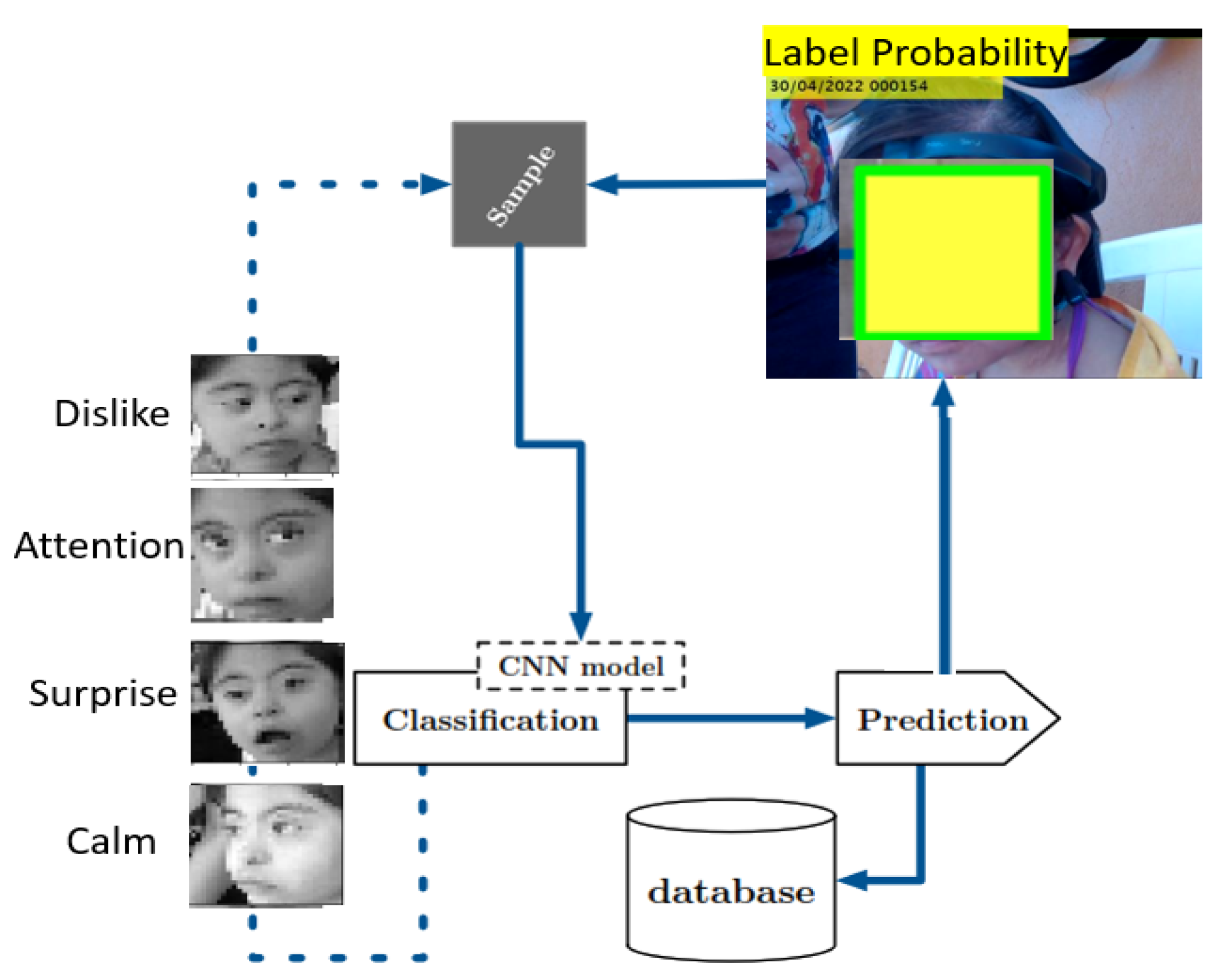
Figure 2 shows the general scheme of our proposal. Thus, this work is based on labeling the emotion a child with Down Syndrome has during dolphin-assisted therapy with high probability. In this figure, it can be observed that emotions are classified by a convolutional neural network model which predicts the possible emotion of the child during the DAT.
The use of exploratory data analysis (EDA) with three folders typically refers to the practice of dividing the dataset into three separate subsets: training, validation, and testing. This partitioning allows for a comprehensive examination of the data and helps in understanding its main characteristics and patterns. The training set is used to teach the deep learning neural network, enabling it to learn from the data. The validation set is employed to fine-tune the model and make adjustments to optimize its performance. Finally, the testing set serves as an independent dataset to assess the model’s generalization and evaluate its accuracy on unseen data. Having these three folders in the EDA process facilitates a robust and thorough analysis of the dataset, ensuring the neural network’s effectiveness and reliability in real-world applications.
In this way, this project uses two datasets, as shown in
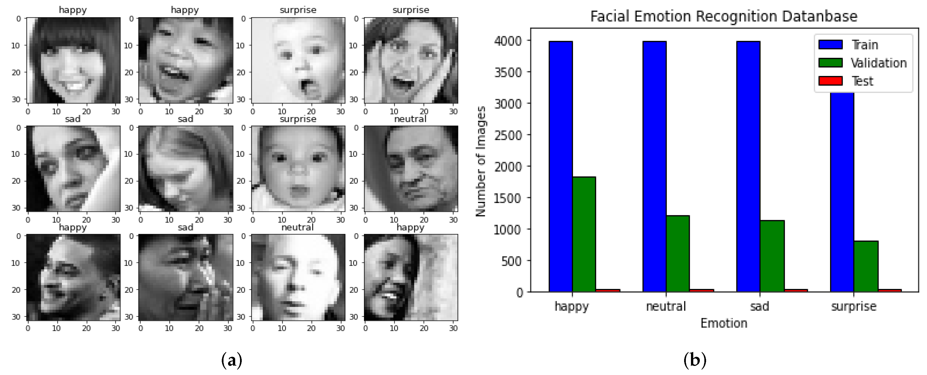
Figure 3. The exploratory data analysis is divided into test, train, and validation. The size of the train dataset is 15,109 images, the test dataset is defined by 128 images, and the validation dataset has 4977 images.
Figure 3a shows a sample of this dataset. Also, in
Figure 3b, the size and distribution of EDA is depicted. This approach involves performing EDA and creating initial models from scratch. During EDA, properties of the input images, classes, and data distribution are examined. The different classes of faces and their characteristics are as follows: happy faces have a smile and eyes somewhat closed with visible teeth, sad faces have eyebrows furrowed and a mouth with the opposite shape of a happy face, neutral faces have no particular expression and share some features with sad faces, and surprised faces have open mouths and eyes wide open, often with hands on the face in many samples.
The testing dataset (128) is smaller than the validation dataset (4977), because the testing dataset serves a different purpose in the model evaluation process. The validation dataset is used for fine-tuning the deep learning neural network and making adjustments to optimize its performance during the training process. It helps in selecting the best model based on its performance on the validation data. On the other hand, the testing dataset is used as an independent dataset to assess the model’s generalization and evaluate its accuracy on unseen data. It is crucial to have a smaller testing dataset to ensure that the model’s performance is not overfitted to a specific subset of data. Using a smaller testing dataset helps in obtaining a more reliable and unbiased estimation of the model’s true performance on new, unseen data. Additionally, the reference to early stopping in the original response suggests that the smaller validation dataset may be used in conjunction with early stopping techniques. Early stopping is a regularization technique that monitors the model’s performance on the validation dataset during training. If the model’s performance on the validation data does not improve or starts to degrade, the training process is halted early to prevent overfitting. This practice is commonly used to avoid training for too many epochs and to find the optimal point at which the model’s generalization is at its best.
In this case, the original training dataset probably had 128 samples, and after applying data augmentation techniques, the dataset expanded to 4977 samples. This augmentation process enhances the neural network’s ability to learn and generalize patterns from the expanded dataset, leading to improved model performance on unseen data during the training process. Furthermore, it addresses the issue of dataset imbalance. After data augmentation, the data distribution in the training dataset increased to 4977 samples, which is significantly larger than the original dataset. Data augmentation is a technique used to artificially increase the size of the training dataset by applying various transformations to existing samples, such as rotations, translations, flips, and changes in brightness and contrast. These transformations create new samples that are variations in the original data, introducing diversity and reducing the risk of overfitting.
Although the class definitions are clear, there are some images that are difficult to classify, such as happy faces that are not smiling and sad faces that are closer to being neutral. This can cause confusion for the model during classification. Additionally, there is an imbalance in the distribution of classes, with fewer images for the surprise class in the training set. This could result in a biased model that struggles to classify surprise faces.
The dataloader used is based on ImageDataGenerator class, which provides images in batches and performs data augmentation through flips, brightness adjustments, and shear operations to increase the number of images and prevent overfitting. Data augmentation is applied to the training, validation, and test sets.
Initially, there was some uncertainty about the appropriate color mode for the images, but it was determined that greyscale was suitable, since the images were found to be in greyscale using
rasterio. However, the first model was constructed using three channels. Greyscale images are often considered better than color images for certain tasks, especially when dealing with limited computational resources and specific image analysis tasks. One of the main advantages of using greyscale images is their reduced data size and complexity. Greyscale images contain only one channel of pixel values (usually representing intensity), whereas color images have multiple channels (e.g., RGB channels) that require more memory and computational resources to process. For tasks that mainly rely on texture or intensity information, such as edge detection, image segmentation, and certain feature extraction tasks, greyscale images can be sufficient and more computationally efficient. Since color information may not always be relevant for such tasks, using greyscale images allows the model to focus on the relevant features and reduce unnecessary noise from color variations. Moreover, in the context of convolutional neural networks (CNNs), using greyscale images can reduce the number of parameters and, thus, the complexity of the model, leading to faster training and inference times. Greyscale CNNs are particularly useful when working with small datasets or resource-constrained environments. However, it is essential to note that the choice between greyscale and color images depends on the specific task and the nature of the data. For tasks that heavily rely on color information, such as object recognition or image classification, color images may provide more relevant features and lead to better performance. The decision to use greyscale or color images should be based on the requirements of the application and the specific characteristics of the dataset [
19].
It is a CNN model with three convolutional blocks and two fully connected layers, with 605,572 parameters, and it was trained for 20 epochs with a batch size of 32 using the Adam optimizer, with a learning rate of 0.001 and categorical cross-entropy as the loss function.
In this way, the final implementation is proposed to implement a Deep Convolutional Neural Network, taking into account the advantages of these kind of architectures. The architectural design of the proposed implementation involves a Deep Convolutional Neural Network (DCNN), leveraging the advantages of such architectures. This DCNN model is structured with various layers, including convolutional, batch normalization, max pooling, and dropout layers. In this way, the presented architecture consists of 6 convolutional layers with ELU activation, followed always by a batch normalization layer. The first two layers have a kernel size of (5,5), while the remaining layers have a kernel size of (3,3). Another distinction is that the first two layers have 64 filters, which are doubled every two layers to reach a total of 256 filters. The model is compiled using the Adam optimizer with a learning rate of 0.001, utilizing categorical cross-entropy as the loss function and accuracy as the metric. This architecture’s goal is to effectively classify data into various classes using the CNN-based approach.
Thus, this DCNN model consists of a total of 2,398,404 parameters. Out of these, 2,396,356 parameters are trainable, meaning they are updated during the training process to optimize the model’s performance. The remaining 2048 parameters are nontrainable, indicating that their values are fixed and do not change during training. These nontrainable parameters might include biases or other fixed elements in the model’s architecture. The combination of trainable and nontrainable parameters contributes to the overall complexity and functionality of the CNN model.
3.2. Adapting Findings in a Down Syndrome Dataset
In
Figure 4, the Second or Down Syndrome Dataset (DSDS) consisting of three folders, i.e., test, train, and validation, is shown.
DSDS also consists in three subsets: (i)
test, (ii)
train, and (iii)
validation. It is important to mention that the images in the DSDS were obtained before, during, and after a female patient diagnosed with Down Syndrome participated in dolphin-assisted therapy. These images were labeled by a psychology expert. The inclusion of each image in the training, validation, or testing category was decided randomly by the same expert. In this way, the size of the Train dataset is 933 images, the Test dataset is defined by 128 images, and the Validation dataset has 384 images.
Figure 4a shows a sample of this dataset.
Figure 4b depicts the size and distribution of the DSDS. Each folder in this dataset has four subfolders:
attention: Images of children with Down Syndrome who were in attention during a DAT.
calm: Images of children with Down Syndrome with calm facial expressions.
dislike: Images of children with Down Syndrome with upset facial expressions.
surprise: Images of children with Down Syndrome who have shocked or surprised facial expressions.
As we can see, the DSDS is smaller than EDA because it is the best architecture found in EDA, and then it is applied in the Down Syndrome Dataset.
Figure 5 shows the QR code in Google Drive, where both the EDA and DSDS can be downloaded.
The performances of the different models on the validation and testing sets are represented in
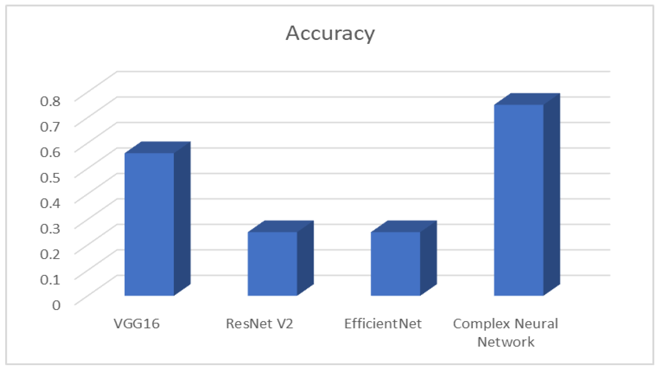
Table 1. As can be seen from the results, the complex neural network architecture achieved the best performance on the validation set, and this complemented the robustness performance, achieving 75% for this image database, as shown in
Figure 6. The VGG16 architecture achieved the second best performance in the validation set with 56%. Finally, EfficientNet and ResNet V2 had the worst robustness accuracy among all the models with only 25% accuracy. In this case, we employ robustness accuracy to refer to the ability of a model or system to maintain high accuracy and performance even when facing challenges, variations, or perturbations in the data or input conditions. In the context of facial emotion recognition, or any other machine learning task, a robust model can handle different lighting conditions, facial expressions, camera angles, and other variations in the input data without significantly compromising its accuracy. A robust model is less sensitive to small changes or noise in the input, making it more reliable and suitable for real-world applications where the data may not always be consistent or perfectly controlled. Evaluating a model’s robustness accuracy helps ensure that it can perform well in various practical scenarios and generalizes effectively to unseen data. Achieving high robustness accuracy is crucial for deploying machine learning systems in real-world settings where variability and uncertainties are inherent.
Thw VGG16, ResNet V2, and EfficientNet neural network models have the following architecture: The first convolutional layer has 24 filters, a kernel size of 3 × 3, and the same padding. The input shape is (32,32,1), with a LeakyRelu layer with a slope of 0.1. The second convolutional layer has 32 filters, a kernel size of 3 × 3, and the same padding, with a LeakyRelu layer with a slope of 0.1, a max pooling layer with a pool size of 2 × 2, and a batch normalization layer. The third convolutional layer has 32 filters, a kernel size of 3 × 3, and the same padding, with a LeakyRelu layer with a slope of 0.1. The fourth convolutional layer has 64 filters, a kernel size of 3 × 3, and the same padding, with a LeakyRelu layer with a slope of 0.1, a max pooling layer with a pool size of 2 × 2, a batch normalization layer, a flatten layer to transform the output from the previous layer, a dense layer with 48 nodes, and a dropout layer with a rate of 0.5. The final output layer has 4 nodes (number of classes) and a softmax activation function. Finally, the model is compiled with categorical cross-entropy loss, Adam optimizer with a learning rate of 0.001, and the metric set to accuracy. The total parameters for VGG16 are 14,714,688; 42,658,176 parameters for ResNet V2; and 8,769,374 parameters for EfficientNet.
This solution designs an architecture of Deep Convolutional Neural Networks. This architecture includes convolutional layers in six blocks, as well as some batch normalization layers. In this model, also called DS-CNN, each convolutional block has one CNN 2D layer, followed by a batch normalization, an ELU activation, and a max pooling 2D layer. For this architecture, any dropout layers with a dropout ratio of 0.4 are defined.
Figure 7 shows the architecture of DS-CNN.
In this way, this model is a sequential model with several convolutional blocks and fully connected layers. The model architecture is as follows: First and sixth CNN blocks consist of a convolutional layer with 256 filters; the second and fifth CNN blocks contain a convolutional layer with 192 filters; and third and fourth CNN blocks comprise a convolutional layer with 128 filters. All six blocks include a kernel size of (2,2) and a relu activation function. The flatten layer flattens the output from the previous layers. The first fully connected layer is a dense layer with 256 units and a relu activation function. The output layer is a dense layer with the number of classes and a softmax activation function. The model is compiled using the Adam optimizer with a learning rate of 0.001. The loss function is categorical cross-entropy, and the metric used for evaluation is accuracy. This architecture aims to classify data into multiple classes using convolutional layers followed by fully connected layers.
The DS-CNN model has a total of 151,653,764 parameters, including both trainable and nontrainable parameters. The trainable parameters are those that are updated during the training process to optimize the model’s performance. In this case, all 151,653,764 parameters are trainable, indicating that the model can learn and adjust the values of these parameters based on the training data. The nontrainable parameters, on the other hand, are fixed and do not change during training. These parameters are usually associated with pretrained layers or frozen layers in the network. In this model, there are no nontrainable parameters, implying that all parameters are adjustable and updated during the training process.
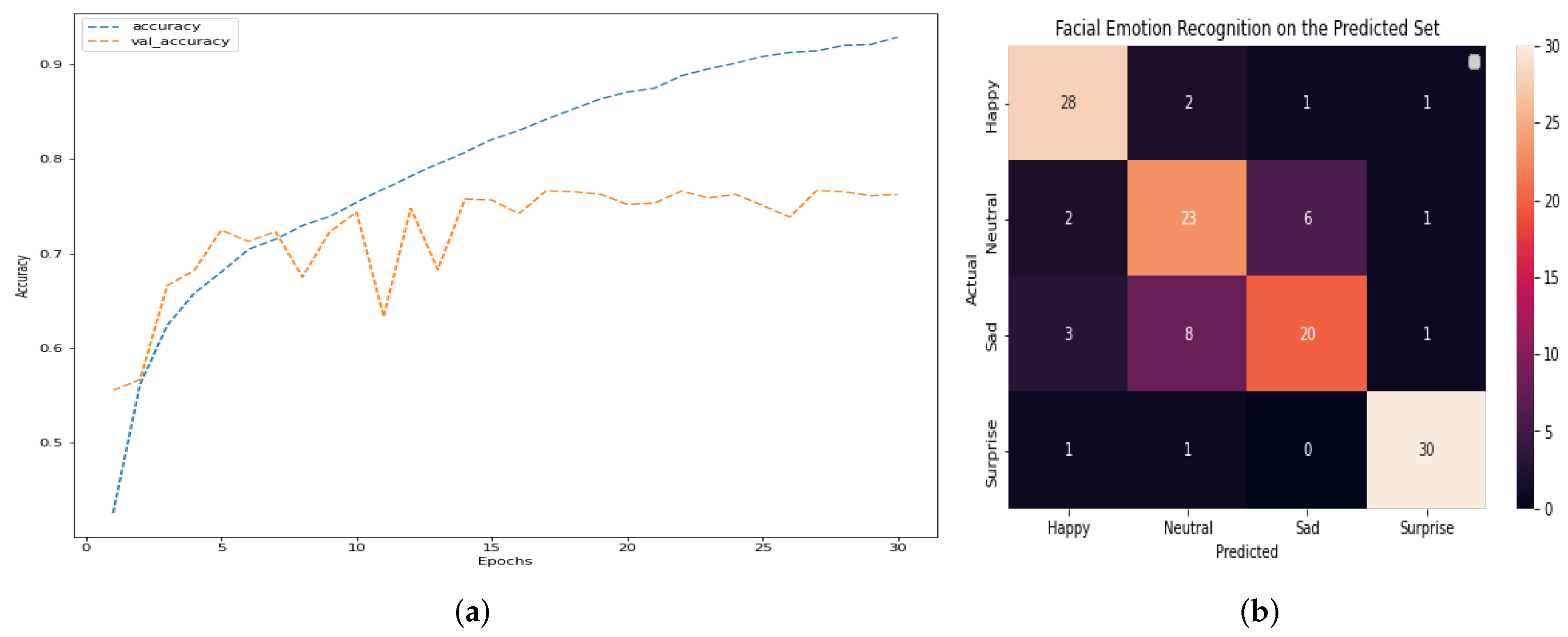
The outcomes of this stage of the project show that DS-CNN does not show overfitting and increases the efficiency regarding other architectures. Overall accuracy reaches 79% and, among the four emotions, surprise is the one that obtains the best results.
Figure 8 shows the main result of DS-CNN.
Figure 8a,b, along with
Table 2, depict, respectively, the accuracy, confusion matrix, and the classification report of the model. The model can be observed to have high percentages of assertiveness and accuracy, with an average of 79%. This indicates that it is a robust model that has significant opportunities for improvement. We can determine if there is no overfitting in a deep learning model by analyzing its performance on both the training and validation datasets. Overfitting occurs when a model performs exceptionally well on the training data but fails to generalize to new, unseen data (validation or test data). If the training and validation accuracies are both high and show similar trends as the model is trained, this points out that the model is not overfitting. To further confirm the absence of overfitting, we can compare the model’s accuracy on the training and validation datasets throughout the training process. If the training accuracy continues to increase while the validation accuracy plateaus or remains stable, it suggests that the model is not memorizing the training data but rather learning to generalize to new data. Running the model for more epochs may lead to better results if there is no overfitting, because the model continues to learn from the training data and improve its performance. However, if overfitting is present, continuing to train the model for more epochs can worsen its generalization capabilities, as it will increasingly memorize the training data and lose the ability to generalize to new data. Finally, by monitoring the training and validation accuracies and ensuring they both perform well without significant divergence, we can conclude that there is no overfitting. In such cases, running the model for more epochs may lead to improved results and better generalization.
The decision to stop early and determine the appropriate number of epochs in
Figure 8 is based on monitoring the model’s performance by using the validation data. Overfitting occurs when a model learns to perform exceptionally well on the training data; however, it fails to generalize unseen data, such as the validation set. To address this concern, we continuously tracked the model’s performance on the validation data during training. If we noticed that the validation performance started to degrade or stagnate while the training performance continued to improve, it indicated a sign of overfitting. In
Figure 8, the decision to stop at epoch 30 is a result of this monitoring process. We observed that the validation performance reached a plateau after epoch 30, suggesting that the model’s ability to generalize was stabilized. Thus, stopping at this point helps prevent overfitting and ensures that the model achieves the best possible performance on unseen data.
3.3. Training of the Convolutional Neural Network through Electroencephalogram
Utilizing EEG signals in a CNN offers promising advantages in the field of brain–computer interfaces (BCIs). EEG provides direct access to the brain’s electrical activity, allowing real-time monitoring and an analysis of cognitive states. By integrating EEG signals into a CNN architecture, we can leverage the temporal and spatial information encoded in the brain signals to enhance the learning and decision-making capabilities of the network. This procedure complements this setup by enabling the network to adapt and optimize its behavior based on feedback and rewards received from the environment. This combination holds the potential to unlock new possibilities in the development of advanced neurotechnologies, such as brain-controlled prosthetics, cognitive enhancement systems, and personalized healthcare applications. Overall, the incorporation of EEG in a CNN framework offers a powerful approach to harness the brain’s capabilities, paving the way for innovative advancements in brain–computer interfaces and human–machine interaction.
In this way, an EEG signal is the measurement of the electricity flowing during the synaptic excitation of dendrites in the pyramidal neurons of the cerebral cortex. When neurons are activated, electricity is produced inside dendrites, generating a magnetic and electric field that is measured with EEG systems. The human head contains different layers (the brain, the skull, and the scalp) for attenuating the signal and adding external and internal noise; thus, only a large group of active neurons can emit a potential to be measured or recorded using surface electrodes [
20]. The electrical activity of the brain can be captured on the scalp, at the base of the skull with the brain exposed, or at deep brain locations. The electrodes that acquire the signal can be superficial, basal, or surgical. For EEG, superficial electrodes are used [
21].
Generally, for the acquisition and recording of the brain’s electrical activity in BCI systems, surface electrodes are used on the scalp. There are several ways to accommodate them, called acquisition systems, or simply arrays, e.g., Illionis, Montreal Aird, Lennox, etc., but the most used for research purposes, and certainly in this study, is the International 10-20 Positioning System [
22].
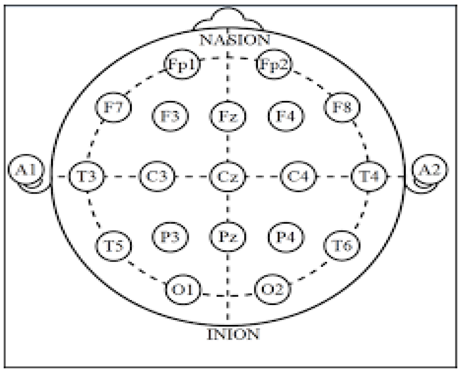
The 10-20 International System is a standardized protocol based on the anatomical references of the inion and nasion longitudinally and the earlobes transversely, ensuring that electrodes are placed on the same areas, regardless of head size. Also, this system is named after its use of 10% or 20% of the anatomically specified distances to place the electrodes, as shown in
Figure 9, from the nasion to the inion and from the earlobes [
23], pointing out that they are the center.
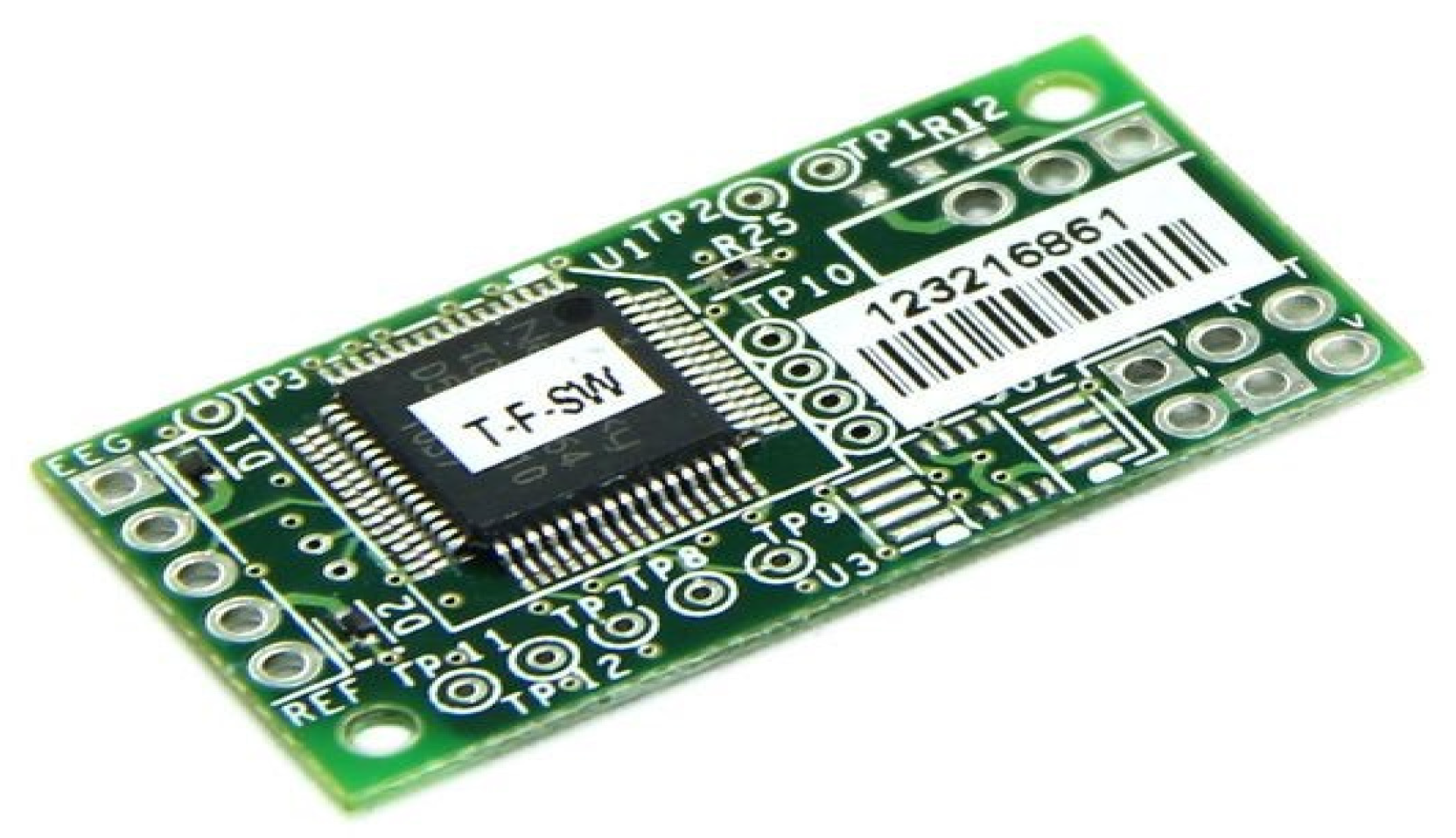
This work uses the EEG device ThinkGear TGAM1, since it collects neural signals and inputs them into the ThinkGear chip for processing the signal into a sequence of usable data and filtering any interference in a digital way. Raw brain signals are amplified and processed to provide concise contributions to the device. The device considered to be the interface between the brain and the computer is the NeuroSky ThinkGear module, shown in
Figure 10, since it meets the requirement of being a noninvasive method, while also having a reliability rate of 98%. The electrode is placed in position
[
24,
25].
The electroencephalographic sample database consists of 124 time-varying samples containing between nine thousand and fifteen thousand records each, with a range between 18 and 30 s.
Table 3 shows a sample of the first 10 brain activity values from both raw signals and preprocessed signals, such as Delta, Theta, Low Alpha, High Alpha, Low Beta, High Beta, Low Gamma, and High Gamma frequency bands (
Figure 11), along with the subject’s percentage of attention (Atte) and meditation (Med) during the test. The EEG sensor TGAM1 sampling rate is 512 samples per second for only the
RAW time series, while the rest of the time series it is one sample per second. It is important to mention that all brain activity rhythms, attention and meditation, are preprocessed within TGAM1 at a rate of 1 Hz, and their equations are proprietary to NeuroSky. Therefore, based on Equation (
1), the RAW signal is converted to microvolts (
) and the power spectral density is calculated.
According to the above, these signals of brain activity are included in the convolutional neural network model, described in
Figure 7, resulting in the model shown in
Figure 12. After testing transfer learning, fine tuning, EEG reinforcement, ensemble model, and recreating DCNN from scratch (even with 1 layer input—greyscale), it was found that fine-tuning can improve the model’s performance. Thirty models were built to test these methods, and the best-performing model was the DCNN with fine-tuning + dense blocks, achieving a testing accuracy of 80%. The model was trained for 30 epochs, using a batch size of 32, the Adam optimizer with a learning rate of 0.001, and the categorical cross-entropy loss function. The structure of the model consisted of two main parts: (i) DCNN with an input shape of
, with 7 first layers frozen and the remaining layers trainable, and (ii) flattening, with three dense blocks with dense layers of 1024 neurons and batch normalization.
It is important to note that there is a very high probability that there is a desynchronization in both datasets, but they could still be used together by aligning their timestamps and ensuring that the data correspond to the same events or time intervals. To use the image and EEG datasets together, the following six steps were taken:
Preprocessing: Preprocess both image and EEG data separately to ensure they are in a compatible format and aligned with the same timestamps or time intervals.
Timestamp Alignment: The data were recorded simultaneously. Despite this, an alignment was made with the timestamps, or the synchronized the datasets were matched to the corresponding events or time periods. This can be achieved through careful data preprocessing and timestamping.
Feature Extraction: Extract relevant features from both datasets, such as facial expressions from images and specific EEG features related to emotions.
Fusion: Combine the features extracted from both datasets to create a unified feature representation that includes both visual and EEG information. This fusion step could involve concatenating the features or using more sophisticated techniques, such as multimodal learning.
Model Training: Train a deep learning model, such as a CNN, on the fused feature representation to recognize facial emotions using the combined information from both image and EEG data.
Evaluation: Evaluate the model’s performance on a validation or test dataset to assess how well it can predict facial emotions based on the joint information from images and EEG.
In summary, it was possible to utilize both datasets together to enhance the model’s understanding of facial emotions and potentially improve the accuracy of the facial emotion recognition task.


 ,
, 


