

Machine Learning Algorithm-Based Prediction of Diabetes Among Female Population Using PIMA Dataset

 , , ,
, , , 
 and
and
Abstract
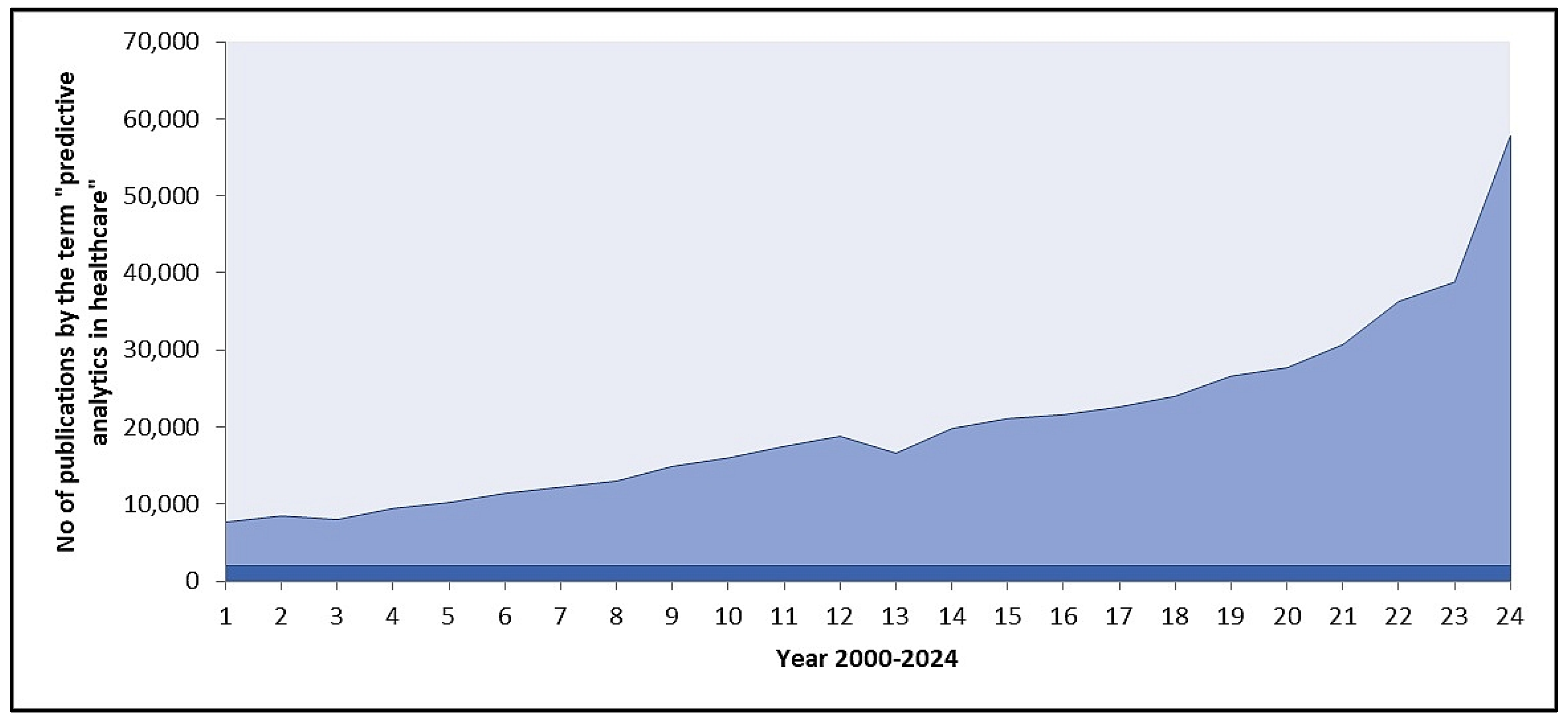
1. Introduction
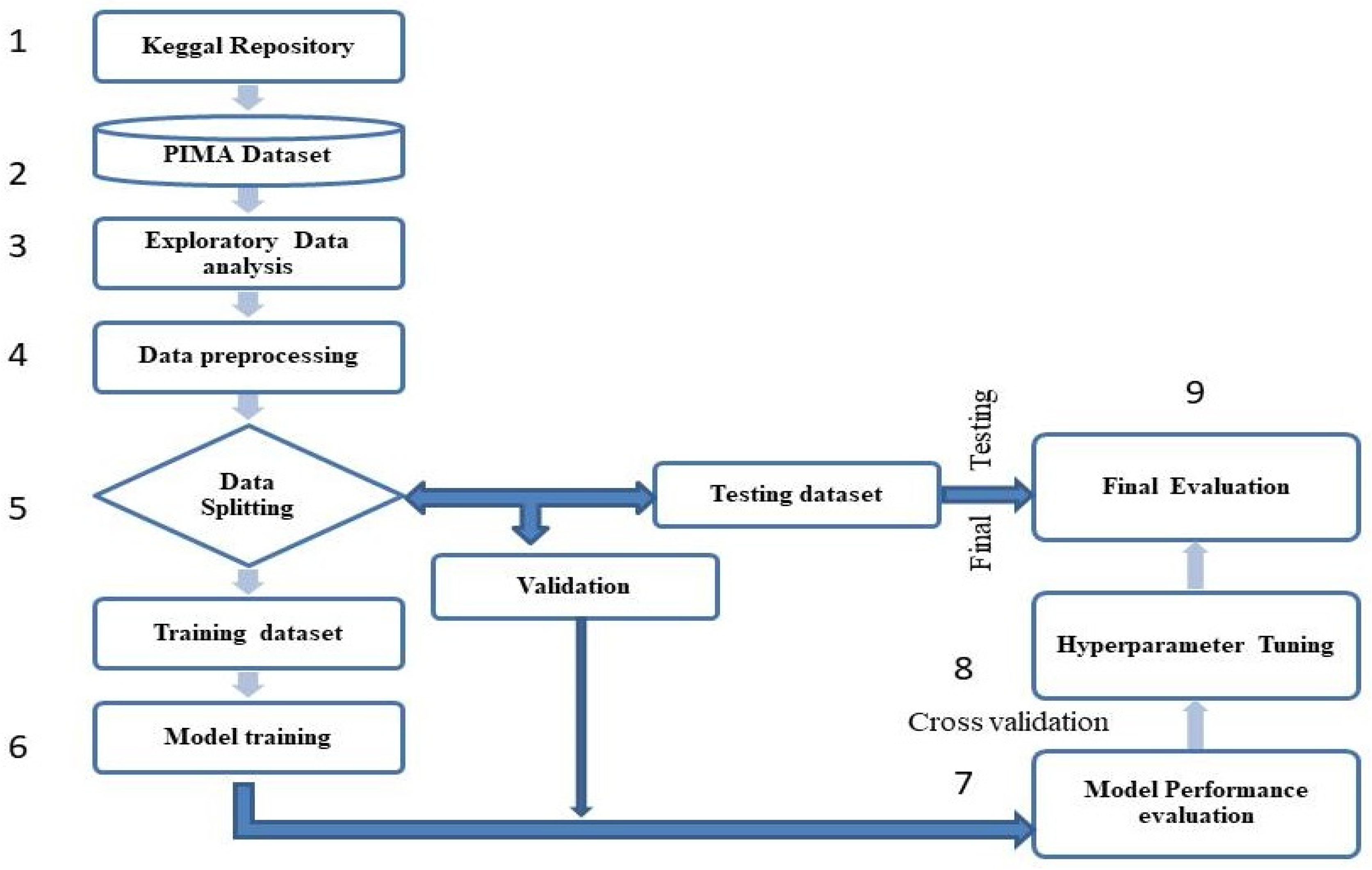
2. Materials and Methods
2.1. Dataset
2.2. Exploratory Data Analysis (EDA)
Data Visualization with PCA
2.3. Pre-Processing
2.3.1. Normalization
2.3.2. Feature Extraction
2.3.3. Dataset Splitting
2.4. ML Models Development
2.5. Model Performance Evaluation
- True Positive (TP): Correctly predicted positive cases.
- False Positive (FP): Incorrectly predicted positive cases (actually negative).
- True Negative (TN): Correctly predicted negative cases.
- False Negative (FN): Incorrectly predicted negative cases (actually positive).
3. Results
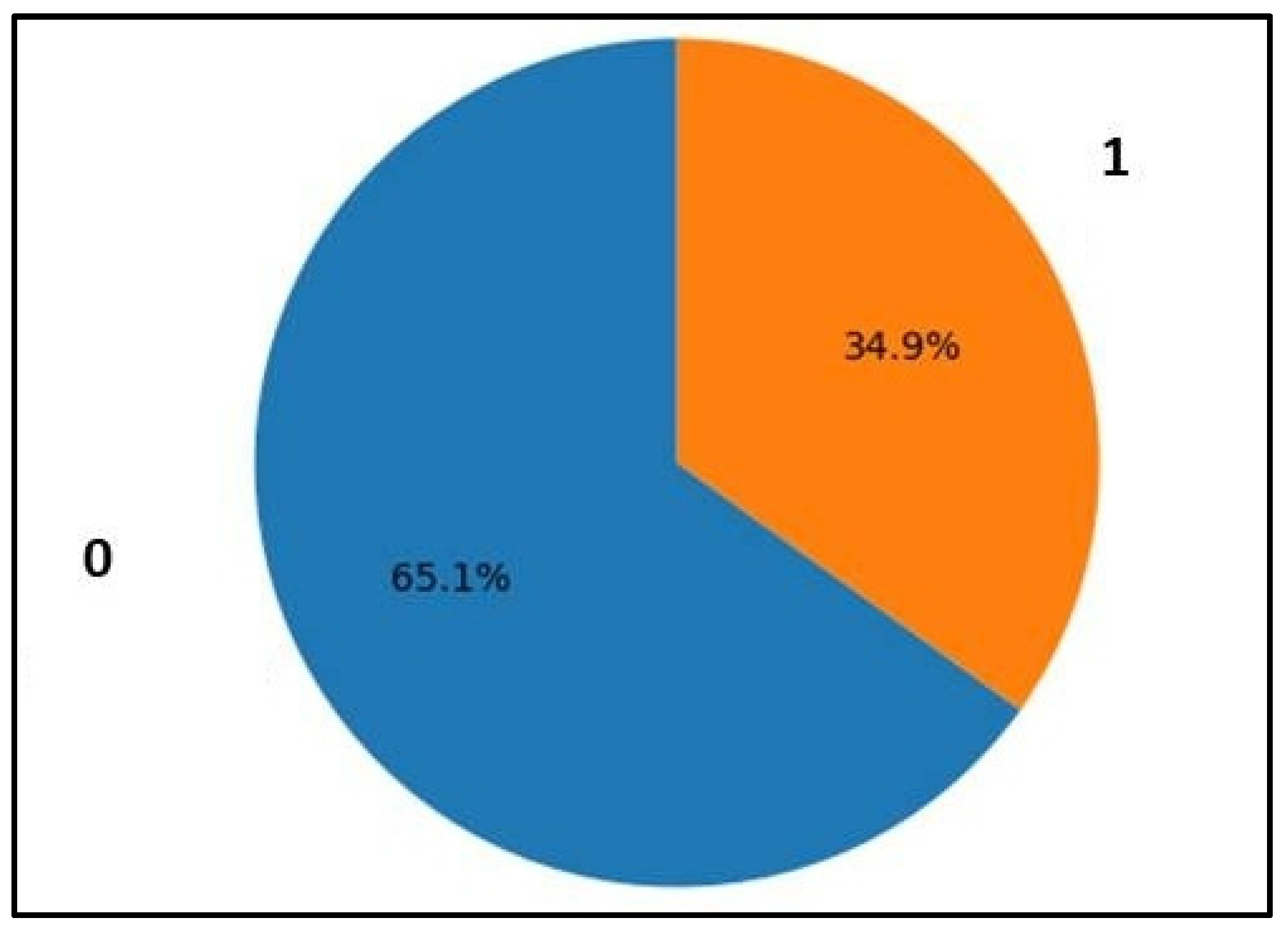
3.1. Dataset Characteristics
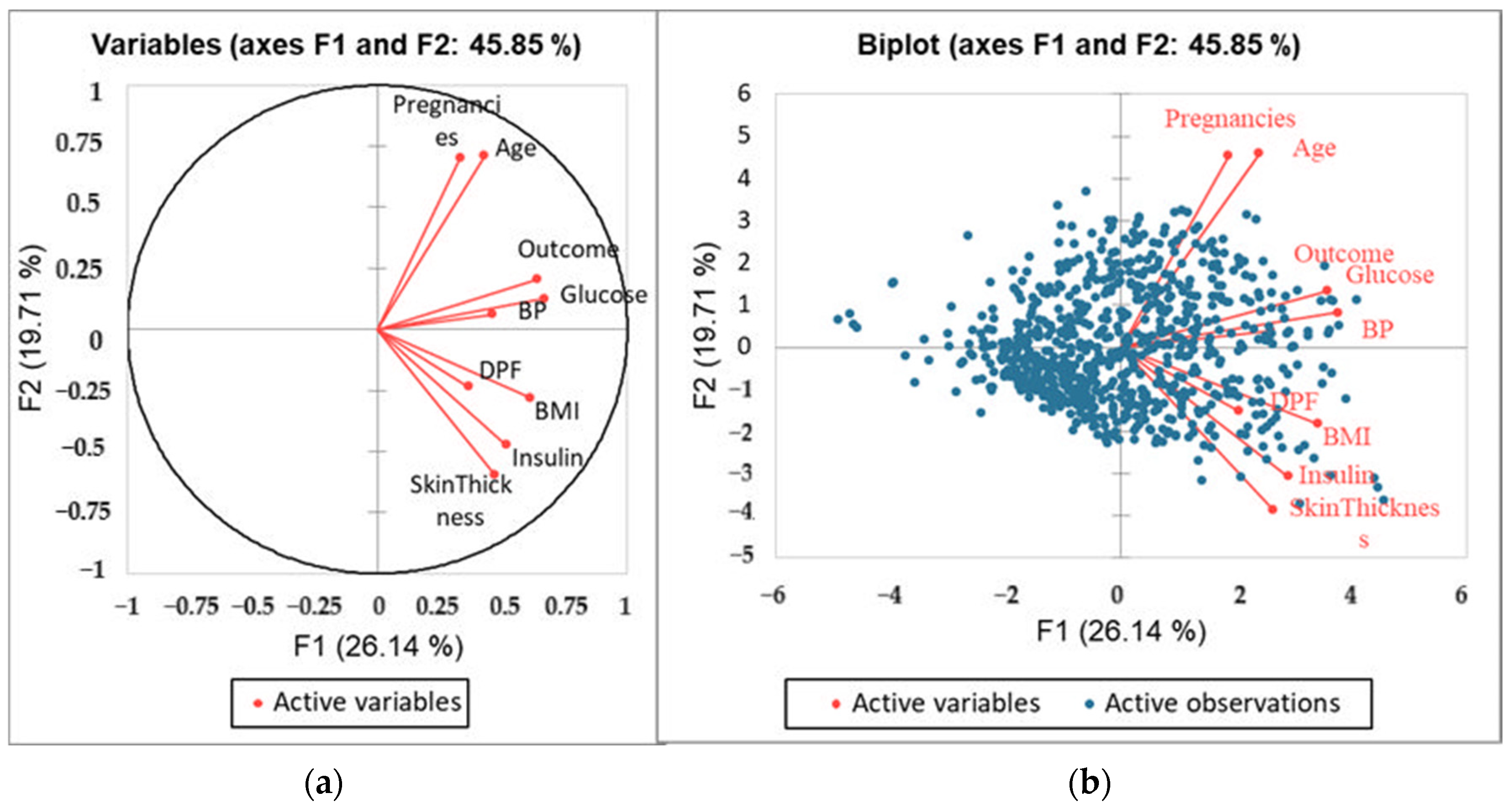
3.2. Principal Component Analysis
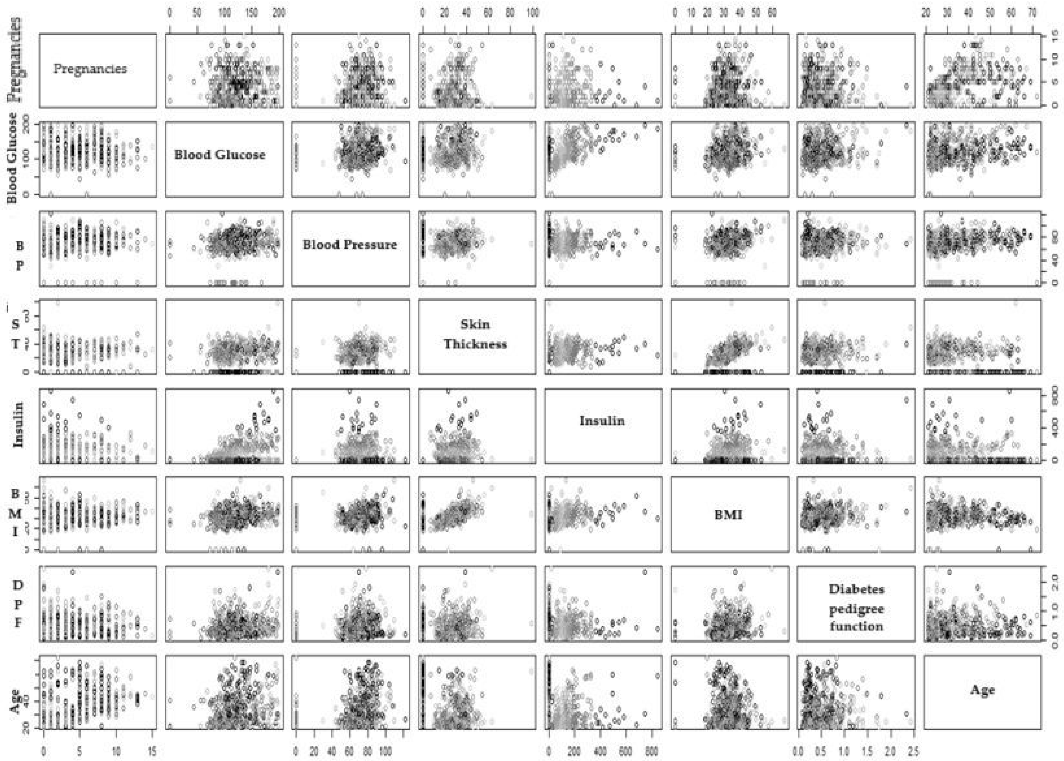
3.3. Scatter Pot
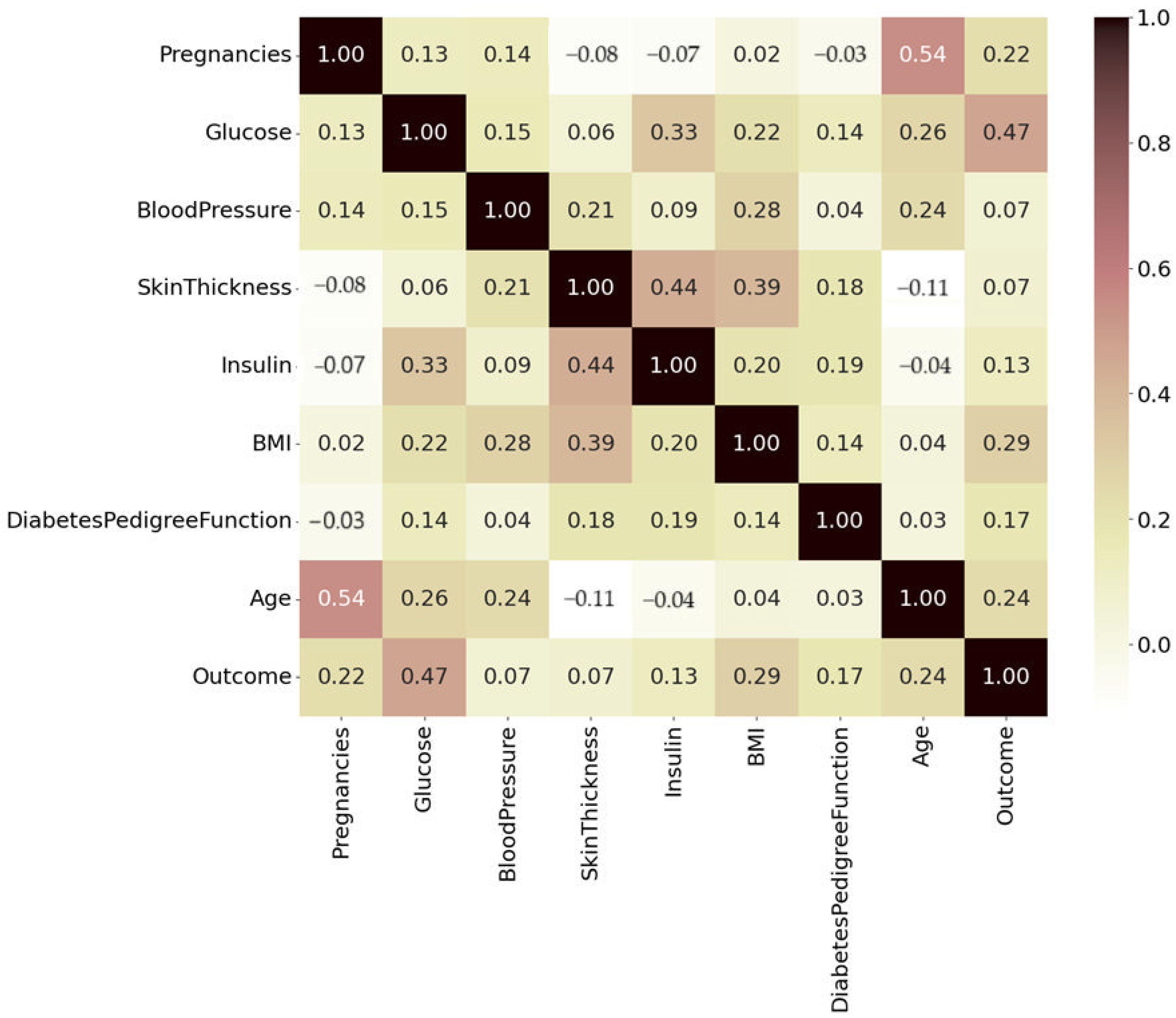
3.4. Correlation Analysis
- Darker shades, dark brown to black, represent strong positive correlations of 0.8 to 1.0.
- Pink and red (0.4 to 0.79) are moderately positive, and lighter shades of pale yellow and white indicate weaker or near-zero correlations (0.2 to 0.39).
- Negative correlations are faint brown.
3.5. ML Models
3.5.1. Decision Tree
3.5.2. Random Forest
3.5.3. Naïve Bayes
3.5.4. Logistic Regression
3.6. ROC Curve
3.7. Cross Validation
- It achieves a balance between computational cost and performance evaluation reliability.
- It provides sufficient training data for each fold, especially for moderately large datasets.
- It is a common practice supported by the literature, particularly in experiments involving iterative tuning or resource constraints.
- Five-fold cross-validation methods are used for small-to-large datasets; in other diabetic research, five-fold CV offers good results [38]. The results obtained in our study are shown in Table 11, and it can be seen that NB has a slightly better average accuracy of 0.76 on the testing dataset as compared to RF 0.75, which is statistically not significant.
4. Conclusions
5. Way Forward
Supplementary Materials
Author Contributions
Funding
Institutional Review Board Statement
Informed Consent Statement
Data Availability Statement
Acknowledgments
Conflicts of Interest
References
- Khan, J.; Sheoran, S.; Khan, W.; Panda, B.P. Metabolic differentiation and quantification of gymnemic acid in Gymnema sylvestre (Retz.) R.Br. ex Sm. leaf extract and its fermented products. Phytochem. Anal. 2020, 31, 488–500. [Google Scholar] [CrossRef] [PubMed]
- Sun, H.; Saeedi, P.; Karuranga, S.; Pinkepank, M.; Ogurtsova, K.; Duncan, B.B.; Stein, C.; Basit, A.; Chan, J.C.N.; Mbanya, J.C.; et al. IDF Diabetes Atlas: Global, regional and country-level diabetes prevalence estimates for 2021 and projections for 2045. Diabetes Res. Clin. Pract. 2022, 183, 109119. [Google Scholar] [CrossRef] [PubMed]
- Wild, S.; Roglic, G.; Green, A.; Sicree, R.; King, H. Estimates for the year 2000 and projections for 2030. Diabetes Care 2004, 27, 1047–1053. [Google Scholar] [CrossRef] [PubMed]
- Cho, N.H.; Shaw, J.E.; Karuranga, S.; Huang, Y.; da Rocha Fernandes, J.D.; Ohlrogge, A.W.; Malanda, B. IDF Diabetes Atlas: Global estimates of diabetes prevalence for 2017 and projections for 2045. Diabetes Res. Clin. Pract. 2018, 138, 271–281. [Google Scholar] [CrossRef]
- Okur, M.E.; Karantas, I.D.; Siafaka, P.I. Diabetes mellitus: A review on pathophysiology, current status of oral medications and future perspectives. ACTA Pharm. Sci. 2017, 55, 1. [Google Scholar]
- Petrie, J.R.; Guzik, T.J.; Touyz, R.M. Diabetes, Hypertension, and Cardiovascular Disease: Clinical Insights and Vascular Mechanisms. Can. J. Cardiol. 2018, 34, 575–584. [Google Scholar] [CrossRef]
- Herman, W.H.; Ye, W.; Griffin, S.J.; Simmons, R.K.; Davies, M.J.; Khunti, K.; Rutten, G.E.H.M.; Sandbaek, A.; Lauritzen, T.; Borch-Johnsen, K.; et al. Early detection and treatment of type 2 diabetes reduce cardiovascular morbidity and mortality: A simulation of the results of the Anglo-Danish-Dutch study of intensive treatment in people with screen-detected diabetes in primary care (ADDITION-Europe). Diabetes Care 2015, 38, 1449–1455. [Google Scholar] [CrossRef] [PubMed]
- Ciarambino, T.; Crispino, P.; Leto, G.; Mastrolorenzo, E.; Para, O.; Giordano, M. Influence of Gender in Diabetes Mellitus and Its Complication. Int. J. Mol. Sci. 2022, 23, 8850. [Google Scholar] [CrossRef]
- Chadalavada, S.; Jensen, M.T.; Aung, N.; Cooper, J.; Lekadir, K.; Munroe, P.B.; Petersen, S.E. Women With Diabetes Are at Increased Relative Risk of Heart Failure Compared to Men: Insights From UK Biobank. Front. Cardiovasc. Med. 2021, 8, 658726. [Google Scholar] [CrossRef]
- Balogh, E.P.; Miller, B.T.; Ball, J.R. Improving Diagnosis in Health Care; National Academies Press: Washington, DC, USA, 2016; ISBN 0309377692. [Google Scholar]
- Mujumdar, A.; Vaidehi, V. Diabetes Prediction using Machine Learning Algorithms. Procedia Comput. Sci. 2019, 165, 292–299. [Google Scholar] [CrossRef]
- Tasin, I.; Nabil, T.U.; Islam, S.; Khan, R. Diabetes prediction using machine learning and explainable AI techniques. Healthc. Technol. Lett. 2023, 10, 1–10. [Google Scholar] [CrossRef] [PubMed]
- Javaid, M.; Haleem, A.; Pratap Singh, R.; Suman, R.; Rab, S. Significance of machine learning in healthcare: Features, pillars and applications. Int. J. Intell. Netw. 2022, 3, 58–73. [Google Scholar] [CrossRef]
- Ahsan, M.M.; Luna, S.A.; Siddique, Z. Machine-Learning-Based Disease Diagnosis: A comprehensive review. Healthcare 2022, 10, 541. [Google Scholar] [CrossRef] [PubMed]
- Afzal, A.H.; Alam, O.; Zafar, S.; Alam, M.A.; Ahmed, K.; Khan, J.; Khan, R.; Shahat, A.A.; Alhalmi, A. Application of Machine Learning for the Prediction of Absorption, Distribution, Metabolism and Excretion (ADME) Properties from Cichorium intybus Plant Phytomolecules. Processes 2024, 12, 2488. [Google Scholar] [CrossRef]
- Vatankhah, M.; Momenzadeh, M. Self-regularized Lasso for selection of most informative features in microarray cancer classification. Multimed. Tools Appl. 2024, 83, 5955–5970. [Google Scholar] [CrossRef]
- Ghaderzadeh, M.; Shalchian, A.; Irajian, G.; Sadeghsalehi, H.; Bialvaei, A.Z.; Sabet, B. Artificial Intelligence in Drug Discovery and Development Against Antimicrobial Resistance: A Narrative Review. Iran. J. Med. Microbiol. 2024, 18, 135–147. [Google Scholar] [CrossRef]
- Sarker, I.H. Machine Learning: Algorithms, Real-World Applications and Research Directions. SN Comput. Sci. 2021, 2, 1–21. [Google Scholar] [CrossRef]
- Pima Indians Diabetes Database. Available online: https://www.kaggle.com/datasets/uciml/pima-indians-diabetes-database (accessed on 19 October 2023).
- Benhar, H.; Idri, A.; Fernández-Alemán, J.L. Data preprocessing for heart disease classification: A systematic literature review. Comput. Methods Programs Biomed. 2020, 195, 105635. [Google Scholar] [CrossRef] [PubMed]
- Kumar, Y.; Koul, A.; Singla, R.; Ijaz, M.F. Artificial intelligence in disease diagnosis: A systematic literature review, synthesizing framework and future research agenda. J. Ambient Intell. Humaniz. Comput. 2023, 14, 8459–8486. [Google Scholar] [CrossRef] [PubMed]
- Nwokoma, F.; Foreman, J.; Akujuobi, C.M. Effective Data Reduction Using Discriminative Feature Selection Based on Principal Component Analysis. Mach. Learn. Knowl. Extr. 2024, 6, 789–799. [Google Scholar] [CrossRef]
- Chang, V.; Ganatra, M.A.; Hall, K.; Golightly, L.; Xu, Q.A. An assessment of machine learning models and algorithms for early prediction and diagnosis of diabetes using health indicators. Healthc. Anal. 2022, 2, 100118. [Google Scholar] [CrossRef]
- Hao, J.; Ho, T.K. Machine learning made easy: A review of scikit-learn package in python programming language. J. Educ. Behav. Stat. 2019, 44, 348–361. [Google Scholar] [CrossRef]
- Sahoo, A.K.; Pradhan, C.; Das, H. Performance Evaluation of Different Machine Learning Methods and Deep-Learning Based Convolutional Neural Network for Health Decision Making. In Nature Inspired Computing for Data Science; Rout, M., Rout, J.K., Das, H., Eds.; Springer International Publishing: Cham, Switzerland, 2020; pp. 201–212. ISBN 978-3-030-33820-6. [Google Scholar]
- Miller, K.W.; Farage, M.A.; Elsner, P.; Maibach, H.I. Characteristics of the Aging Skin. Adv. Wound Care 2013, 2, 5–10. [Google Scholar] [CrossRef]
- Rawal, G.; Yadav, S. Glycosylated hemoglobin (HbA1C): A brief overview for clinicians. Indian J. Immunol. Respir. Med. 2016, 1, 33–36. [Google Scholar]
- Rodriguez, B.S.Q.; Vadakekut, E.S.; Mahdy, H. Gestational diabetes. In StatPearls; StatPearls Publishing: Treasure Island, FL, USA, 2024. [Google Scholar]
- Ong, K.K.; Diderholm, B.; Salzano, G.; Wingate, D.; Hughes, I.A.; MacDougall, J.; Acerini, C.L.; Dunger, D.B. Pregnancy insulin, glucose, and BMI contribute to birth outcomes in nondiabetic mothers. Diabetes Care 2008, 31, 2193–2197. [Google Scholar] [CrossRef]
- Smallman, L.; Artemiou, A.; Morgan, J. Sparse Generalised Principal Component Analysis. Pattern Recognit. 2018, 83, 443–455. [Google Scholar] [CrossRef]
- Saha, D.; Manickavasagan, A. Machine learning techniques for analysis of hyperspectral images to determine quality of food products: A review. Curr. Res. Food Sci. 2021, 4, 28–44. [Google Scholar] [CrossRef]
- Chang, V.; Bailey, J.; Xu, Q.A.; Sun, Z. Pima Indians diabetes mellitus classification based on machine learning (ML) algorithms. Neural Comput. Appl. 2023, 35, 16157–16173. [Google Scholar] [CrossRef] [PubMed]
- De Tata, V. Age-related impairment of pancreatic beta-cell function: Pathophysiological and cellular mechanisms. Front. Endocrinol. 2014, 5, 1–8. [Google Scholar] [CrossRef] [PubMed]
- Sabu, G.S.; Romi, S.; Sajey, P.S. Microanatomy of Age Related Changes in Epidermal Thickness of Human Male Skin: A Cadaveric Study. Int. J. Pharm. Clin. Res. 2024, 16, 291–297. [Google Scholar]
- Wang, Y.; Zhang, Y.; Zhao, W.; Cai, W.; Zhao, C. Exploring the association between grip strength and adverse pregnancy and perinatal outcomes: A Mendelian randomization study. Heliyon 2024, 10, e33465. [Google Scholar] [CrossRef] [PubMed]
- Mandrekar, J.N. Receiver Operating Characteristic Curve in Diagnostic Test Assessment. J. Thorac. Oncol. 2010, 5, 1315–1316. [Google Scholar] [CrossRef] [PubMed]
- Çorbacıoğlu, Ş.K.; Aksel, G. Receiver operating characteristic curve analysis in diagnostic accuracy studies: A guide to interpreting the area under the curve value. Turk. J. Emerg. Med. 2023, 23, 195–198. [Google Scholar] [CrossRef] [PubMed]
- Nti, I.K.; Nyarko-Boateng, O.; Aning, J. Performance of Machine Learning Algorithms with Different K Values in K-fold CrossValidation. Int. J. Inf. Technol. Comput. Sci. 2021, 13, 61–71. [Google Scholar] [CrossRef]


| Attributes | Inference |
|---|---|
| Pregnancies | Number of times the person has been pregnant |
| Blood Glucose | Blood glucose level on testing |
| Blood Pressure | Diastolic blood pressure |
| Skin Thickness | Skin fold thickness of the triceps |
| Insulin | Amount of insulin in a 2 h serum test |
| BMI | Body mass index |
| DPF | DPF calculates a score that represents the likelihood of diabetes influenced by hereditary factors. |
| Age | Age of the person |
| Outcome | The person is predicted to have diabetes or not |
| Predicted Positive | Predicted Negative | |
|---|---|---|
| Actual positive | True positive | False negative |
| Actual negative | False positive | True negative |
| Pregnancies | Glucose | Blood Pressure | Skin Thickness | Insulin | BMI | DPF | Age | |
|---|---|---|---|---|---|---|---|---|
| Count | 768 | 768 | 768 | 768 | 768 | 768 | 768 | 768 |
| Mean | 3.84 | 121.60 | 72.20 | 26.60 | 118.68 | 32.4 | 0.47 | 33.24 |
| std | 3.36 | 30.40 | 12.10 | 9.60 | 93.08 | 6.80 | 0.33 | 11.76 |
| Min | 0.00 | 44.00 | 24.00 | 7.00 | 14.00 | 18.20 | 0.07 | 21.00 |
| 25% | 1.00 | 99.70 | 64.00 | 20.50 | 79.70 | 27.50 | 0.24 | 24.00 |
| 50% | 3.00 | 117.00 | 72.00 | 23.00 | 79.70 | 32.0 | 0.37 | 29.00 |
| 75% | 6.00 | 140.25 | 80.00 | 32.00 | 127.25 | 36.60 | 0.62 | 41.00 |
| max | 17.00 | 199.00 | 122.00 | 99.00 | 846.00 | 67.10 | 2.42 | 81.00 |
| F1 | F2 | F3 | F4 | F5 | F6 | F7 | F8 | F9 | |
|---|---|---|---|---|---|---|---|---|---|
| Eigenvalue | 2.353 | 1.774 | 1.120 | 0.882 | 0.845 | 0.735 | 0.488 | 0.418 | 0.385 |
| Variability (%) | 26.139 | 19.715 | 12.447 | 9.799 | 9.385 | 8.165 | 5.427 | 4.646 | 4.277 |
| Cumulative % | 26.139 | 45.853 | 58.300 | 68.100 | 77.485 | 85.650 | 91.077 | 95.723 | 100.000 |
| F1 | F2 | F3 | F4 | F5 | |
|---|---|---|---|---|---|
| Pregnancies | 0.110 | 0.494 | 0.030 | 0.023 | 0.038 |
| Glucose | 0.449 | 0.016 | 0.172 | 0.094 | 0.010 |
| Blood Pressure | 0.212 | 0.004 | 0.444 | 0.000 | 0.003 |
| Skin Thickness | 0.222 | 0.357 | 0.097 | 0.005 | 0.025 |
| Insulin | 0.266 | 0.224 | 0.022 | 0.008 | 0.357 |
| BMI | 0.371 | 0.078 | 0.071 | 0.023 | 0.235 |
| DPF | 0.133 | 0.054 | 0.091 | 0.673 | 0.021 |
| Age | 0.183 | 0.504 | 0.018 | 0.026 | 0.035 |
| Outcome | 0.406 | 0.043 | 0.174 | 0.029 | 0.121 |
| Predicted Positive | Predicted Negative | |
|---|---|---|
| Actual positive | 119 | 28 |
| Actual negative | 37 | 47 |
| Negative Positive | Predicted Negative | |
|---|---|---|
| Actual positive | 129 | 18 |
| Actual negative | 29 | 55 |
| Predicted Positive | Predicted Negative | |
|---|---|---|
| Actual positive | 127 | 20 |
| Actual negative | 33 | 51 |
| Predicted Positive | Predicted Negative | |
|---|---|---|
| Actual positive | 114 | 33 |
| Actual negative | 35 | 49 |
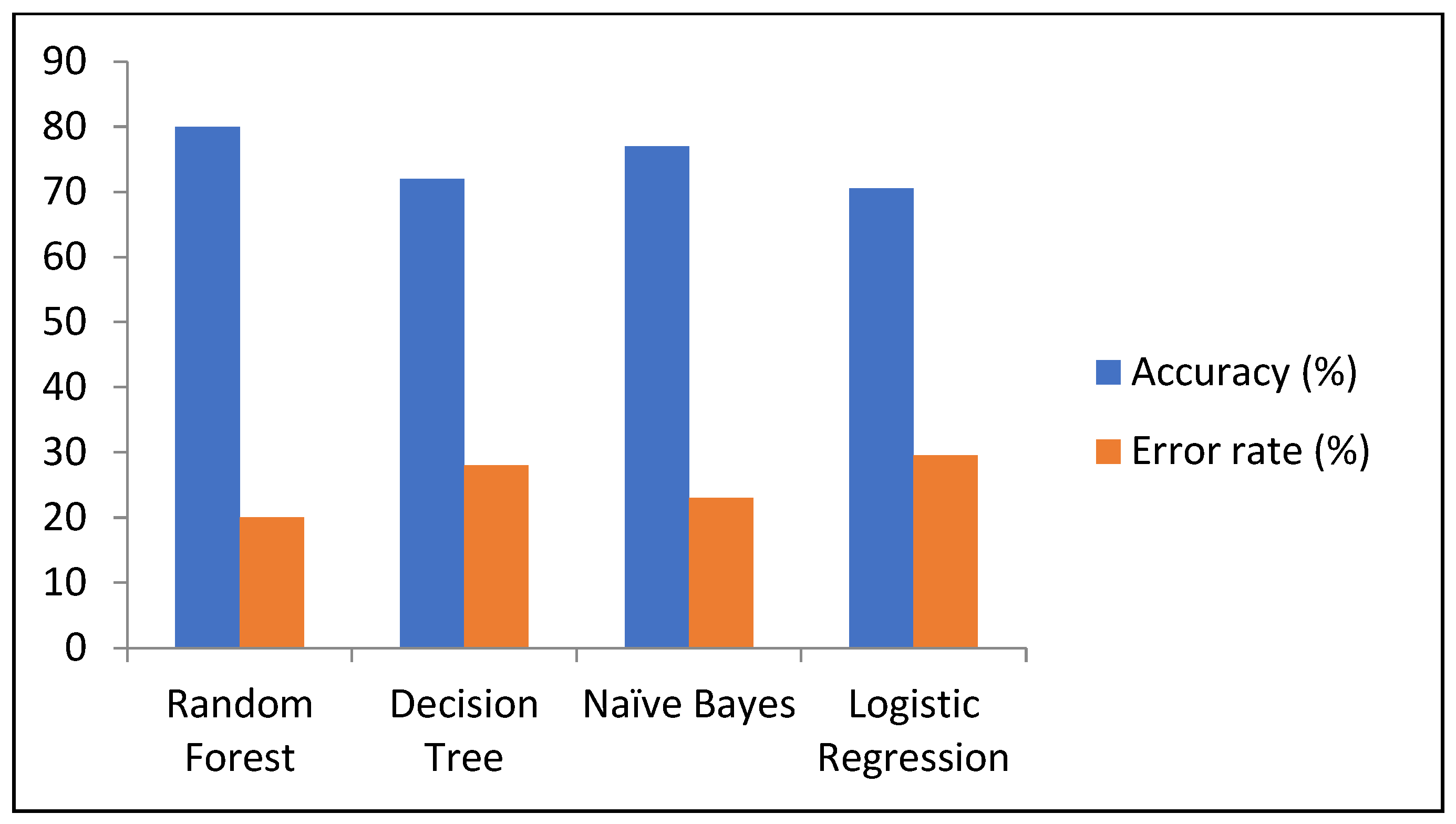
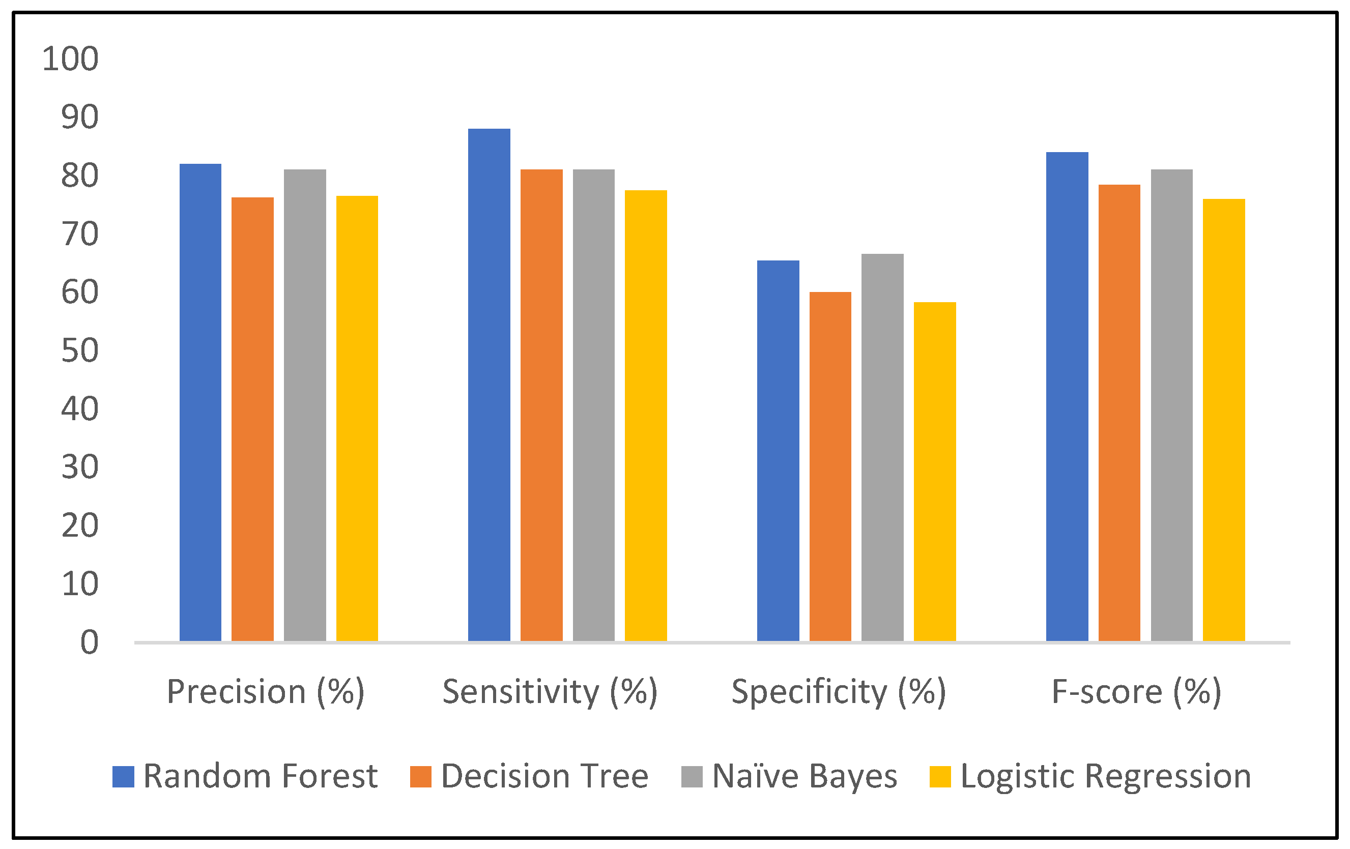
| Model | Accuracy (%) | Precision (%) | Sensitivity (%) | Specificity (%) | F-Score (%) | Error Rate (%) |
|---|---|---|---|---|---|---|
| RF | 80 | 82 | 88 | 65.4 | 84 | 20 |
| DT | 72 | 76.2 | 81 | 60 | 78.4 | 28 |
| NB | 77 | 81 | 81 | 66.6 | 81 | 23 |
| LR | 70.5 | 76.5 | 77.5 | 58.3 | 76 | 29.5 |
| Algorithms | Training Dataset | Testing Dataset | ||||||||||
|---|---|---|---|---|---|---|---|---|---|---|---|---|
| K-1 | K-2 | K-3 | K-4 | K-5 | Avg | K-1 | K-2 | K-3 | K-4 | K-5 | Avg | |
| RF | 0.75 | 0.70 | 0.78 | 0.71 | 0.75 | 0.74 | 0.72 | 0.82 | 0.71 | 0.76 | 0.71 | 0.75 |
| DT | 0.68 | 0.72 | 0.71 | 0.71 | 0.72 | 0.71 | 0.59 | 0.78 | 0.69 | 0.78 | 0.71 | 0.71 |
| NB | 0.78 | 0.69 | 0.76 | 0.72 | 0.73 | 0.74 | 0.78 | 0.78 | 0.73 | 0.73 | 0.76 | 0.76 |
| LR | 0.84 | 0.72 | 0.78 | 0.72 | 0.76 | 0.76 | 0.76 | 0.76 | 0.67 | 0.69 | 0.73 | 0.72 |
Disclaimer/Publisher’s Note: The statements, opinions and data contained in all publications are solely those of the individual author(s) and contributor(s) and not of MDPI and/or the editor(s). MDPI and/or the editor(s) disclaim responsibility for any injury to people or property resulting from any ideas, methods, instructions or products referred to in the content. |
© 2024 by the authors. Licensee MDPI, Basel, Switzerland. This article is an open access article distributed under the terms and conditions of the Creative Commons Attribution (CC BY) license (https://creativecommons.org/licenses/by/4.0/).
Share and Cite
Ahmed, A.; Khan, J.; Arsalan, M.; Ahmed, K.; Shahat, A.A.; Alhalmi, A.; Naaz, S. Machine Learning Algorithm-Based Prediction of Diabetes Among Female Population Using PIMA Dataset. Healthcare 2025, 13, 37. https://doi.org/10.3390/healthcare13010037
Ahmed A, Khan J, Arsalan M, Ahmed K, Shahat AA, Alhalmi A, Naaz S. Machine Learning Algorithm-Based Prediction of Diabetes Among Female Population Using PIMA Dataset. Healthcare. 2025; 13(1):37. https://doi.org/10.3390/healthcare13010037
Chicago/Turabian StyleAhmed, Afshan, Jalaluddin Khan, Mohd Arsalan, Kahksha Ahmed, Abdelaaty A. Shahat, Abdulsalam Alhalmi, and Sameena Naaz. 2025. "Machine Learning Algorithm-Based Prediction of Diabetes Among Female Population Using PIMA Dataset" Healthcare 13, no. 1: 37. https://doi.org/10.3390/healthcare13010037
APA StyleAhmed, A., Khan, J., Arsalan, M., Ahmed, K., Shahat, A. A., Alhalmi, A., & Naaz, S. (2025). Machine Learning Algorithm-Based Prediction of Diabetes Among Female Population Using PIMA Dataset. Healthcare, 13(1), 37. https://doi.org/10.3390/healthcare13010037