
Adolescent Obesity Modeling: A Framework of Socio-Economic Analysis on Public Health

 ,
,  ,
, 
Abstract
:1. Introduction
1.1. Previous Studies on Adolescent Obesity Modeling
1.2. Research Framework and Contributions of the Study
2. Materials and Methods
Sampling Procedure
3. Results
3.1. Descriptive Statistics Analysis
3.2. SEM Analysis
3.2.1. Reliability and Validity Indices
3.2.2. Fitting Model Analysis
3.2.3. Structural Model
3.3. Moderation Analysis
4. Discussion
5. Conclusions
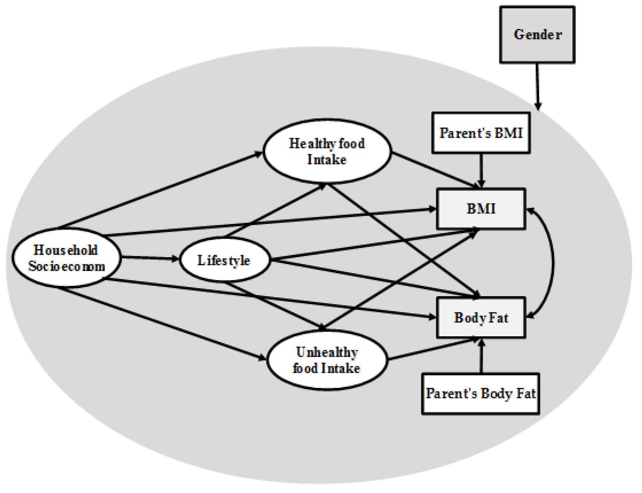
- This study is an improvement of previous research on adolescent obesity modeling because we introduced a new framework (Figure 1) that includes four latent variables and five measurement variables. Another novel contribution of the present study is the inclusion of body fat as the second dependent variable in our research framework—something that has never been done before. To our knowledge, the present study was the first to examine this relationship in adolescent obesity modeling.
- The Bayesian estimator proposed the analysis of convenient structural equations for adolescent obesity modeling. In formulating SEM-ML and SEM-PLS in developing the Bayesian estimator, emphasis was placed on raw individual random observations rather than on the sample covariance and partial least square matrices.
- Some other variables were not included in our research framework such as the economic, political and cultural determinants. They might, however, have a direct or indirect impact on household socioeconomic status and eating behavior. Furthermore, since our data were collected from Tehran, Iran, this makes the economic background a controlling factor in our research framework for adolescent obesity modeling. As such, our data may be representative of the urban Tehran population. Therefore, it is of particular importance that the proposed framework is employed in future research so that these findings can be replicated and extended in other areas and provinces across Iran and other countries.
- Based on previous research, smoking [64,65], alcohol consumption [66,67,68] and genetics [69] were identified as significant indicators of obesity prevalence among adolescents, and hence should be included in the research framework. In the present study, however, we faced certain limitations to obtain data concerning these factors. For instance, more than 70% of participants did not respond to smoking habits and alcohol consumption. Therefore, we were not able to involve these two factors in our research model. Furthermore, genetic factors require DNA analysis based on a blood test that may incur high costs; however, we had a limited budget to involve a clinical test. Therefore, we suggest that future researchers include them in future studies in order to give more credence to our research framework and bolster the evidence of household socioeconomic status, lifestyle and eating behavior in adolescent obesity modeling.
- The present study was limited to cross-sectional data structure and unable to determine any temporal associations between the variables of interest. Future research should thus incorporate longitudinal data that would permit more accuracy and confidence in data analysis with more definitive conclusions regarding adolescent obesity modeling.
Supplementary Materials
Author Contributions
Funding
Institutional Review Board Statement
Informed Consent Statement
Data Availability Statement
Acknowledgments
Conflicts of Interest
References
- Abarca-Gómez, L.; Abdeen, Z.A.; Hamid, Z.A.; Abu-Rmeileh, N.M.; Acosta-Cazares, B.; Acuin, C.; Adams, R.J.; Aekplakorn, W.; Afsana, K.; Aguilar-Salinas, C.A. Worldwide trends in body-mass index, underweight, overweight, and obesity from 1975 to 2016: A pooled analysis of 2416 population-based measurement studies in 1289 million children, adolescents, and adults. Lancet 2017, 390, 2627–2642. [Google Scholar] [CrossRef] [Green Version]
- Martin, M.A. What is the causal effect of income gains on youth obesity? Leveraging the economic boom created by the Marcellus Shale development. Soc. Sci. Med. 2021, 272, 113732. [Google Scholar] [CrossRef] [PubMed]
- Blüher, M. Obesity: Global epidemiology and pathogenesis. Nat. Rev. Endocrinol. 2019, 15, 288–298. [Google Scholar] [CrossRef] [PubMed]
- Organization, W.H. Report of the Commission on Ending Childhood Obesity; WHO Press: Geneva, Switzerland, 2016. [Google Scholar]
- Woo, J.G.; Zhang, N.; Fenchel, M.; Jacobs, D.R.; Hu, T.; Urbina, E.M.; Burns, T.L.; Raitakari, O.; Steinberger, J.; Bazzano, L. Prediction of adult class II/III obesity from childhood BMI: The i3C consortium. Int. J. Obes. 2020, 44, 1164–1172. [Google Scholar] [CrossRef]
- Al-Saadi, L.S.; Ali, A.; Waly, M.I.; Al-Zuhaibi, K. Impact of Dietary Patterns and Nutritional Status on the Academic Performance of Omani School Students. J. Pharm. Nutr. Sci. 2020, 10, 74–87. [Google Scholar]
- Tsang, T.W.; Kohn, M.R.; Chow, C.M.; Singh, M.F. Self-perception and attitude toward physical activity in overweight/obese adolescents: The “martial fitness” study. Res. Sports Med. 2013, 21, 37–51. [Google Scholar] [CrossRef] [PubMed]
- Shore, S.M.; Sachs, M.L.; Lidicker, J.R.; Brett, S.N.; Wright, A.R.; Libonati, J.R.J.O. Decreased scholastic achievement in overweight middle school students. Obesity 2008, 16, 1535–1538. [Google Scholar] [CrossRef]
- Cate, P.-T.; Samouda, H.; Schierloh, U.; Jacobs, J.; Vervier, J.F.; Stranges, S.; Lair, M.L.; De Beaufort, C.J.B.O. Can health indicators and psychosocial characteristics predict attrition in youth with overweight and obesity seeking ambulatory treatment? Data from a retrospective longitudinal study in a paediatric clinic in Luxembourg. BMJ Open 2017, 7. [Google Scholar] [CrossRef] [Green Version]
- Felix, J.; Stark, R.; Teuner, C.; Leidl, R.; Lennerz, B.; Brandt, S.; von Schnurbein, J.; Moss, A.; Bollow, E.; Sergeyev, E. Health related quality of life associated with extreme obesity in adolescents–results from the baseline evaluation of the YES-study. Health Qual. Life Outcomes 2020, 18, 1–11. [Google Scholar] [CrossRef]
- Gross, A.C.; Kaizer, A.M.; Ryder, J.R.; Fox, C.K.; Rudser, K.D.; Dengel, D.R.; Kelly, A.S. Relationships of Anxiety and Depression with Cardiovascular Health in Youth with Normal Weight to Severe Obesity. J. Pediatr. 2018, 199, 85–91. [Google Scholar] [CrossRef]
- Hales, C.M.; Fryar, C.D.; Carroll, M.D.; Freedman, D.S.; Ogden, C.L.J.J. Trends in obesity and severe obesity prevalence in US youth and adults by sex and age, 2007–2008 to 2015–2016. JAMA 2018, 319, 1723–1725. [Google Scholar] [CrossRef] [PubMed] [Green Version]
- Xue, H.; Slivka, L.; Igusa, T.; Huang, T.; Wang, Y. Applications of systems modelling in obesity research. Obes. Rev. 2018, 19, 1293–1308. [Google Scholar] [CrossRef]
- Meisel, J.D.; Ramirez, A.M.; Esguerra, V.; Montes, F.; Stankov, I.; Sarmiento, O.L.; Valdivia, J.A. Using a system dynamics model to study the obesity transition by socioeconomic status in Colombia at the country, regional and department levels. BMJ Open 2020, 10, e036534. [Google Scholar] [CrossRef] [PubMed]
- Hendrie, G.A.; Coveney, J.; Cox, D.N. Defining the complexity of childhood obesity and related behaviours within the family environment using structural equation modelling. Public Health Nutr. 2012, 15, 48–57. [Google Scholar] [CrossRef] [PubMed] [Green Version]
- Lim, S.Y.; da Conceição, L.M.; Camorlinga, S.G. A Study on the Modeling of Obesity. In Embracing Complexity in Health; Springer: Berlin/Heidelberg, Germany, 2019; pp. 307–320. [Google Scholar]
- Lhachimi, S.; Nusselder, W.; Lobstein, T.; Smit, H.; Baili, P.; Bennett, K.; Kulik, M.; Jackson-Leach, R.; Boshuizen, H.; Mackenbach, J. Modelling obesity outcomes: Reducing obesity risk in adulthood may have greater impact than reducing obesity prevalence in childhood. Obes. Rev. 2013, 14, 523–531. [Google Scholar] [CrossRef]
- Mireku, M.O.; Rodriguez, A. Family income gradients in adolescent obesity, overweight and adiposity persist in extremely deprived and extremely affluent neighbourhoods but not in middle-class neighbourhoods: Evidence from the UK Millennium Cohort Study. Int. J. Environ. Res. Public Health 2020, 17, 418. [Google Scholar] [CrossRef] [Green Version]
- Sigmund, E.; Sigmundová, D.; Badura, P.; Voráčová, J.; Vladimír, H.; Hollein, T.; Pavelka, J.; Půžová, Z.; Kalman, M. Time-trends and correlates of obesity in Czech adolescents in relation to family socioeconomic status over a 16-year study period (2002–2018). BMC Public Health 2020, 20, 1–12. [Google Scholar] [CrossRef] [PubMed]
- Tee, J.Y.H.; Gan, W.Y.; Tan, K.-A.; Chin, Y.S. Obesity and unhealthy lifestyle associated with poor executive function among Malaysian adolescents. PLoS ONE 2018, 13, e0195934. [Google Scholar] [CrossRef] [Green Version]
- Micklesfield, L.K.; Hanson, S.K.; Lobelo, F.; Cunningham, S.A.; Hartman, T.J.; Norris, S.A.; Stein, A.D. Adolescent physical activity, sedentary behavior and sleep in relation to body composition at age 18 years in urban South Africa, Birth-to-Twenty+ Cohort. BMC Pediatrics 2021, 21, 1–13. [Google Scholar] [CrossRef]
- Gillis, B.T.; Shimizu, M.; Philbrook, L.E.; El-Sheikh, M. Racial disparities in adolescent sleep duration: Physical activity as a protective factor. Cult. Divers. Ethn. Minority Psychol. 2020, 27, 118–122. [Google Scholar] [CrossRef]
- Fomby, P.; Goode, J.A.; Truong-Vu, K.-P.; Mollborn, S. Adolescent technology, sleep, and physical activity time in two US cohorts. Youth Soc. 2021, 53, 585–609. [Google Scholar] [CrossRef] [PubMed]
- Laurson, K.R.; Lee, J.A.; Eisenmann, J.C. The cumulative impact of physical activity, sleep duration, and television time on adolescent obesity: 2011 Youth Risk Behavior Survey. J. Phys. Act. Health 2015, 12, 355–360. [Google Scholar] [CrossRef] [PubMed]
- Bugge, A.B. Food advertising towards children and young people in Norway. Appetite 2016, 98, 12–18. [Google Scholar] [CrossRef]
- Chai, L.; Xue, J.; Han, Z. The effects of alcohol and tobacco use on academic performance among Chinese children and adolescents: Assessing the mediating effect of skipping class. Child. Youth Serv. Rev. 2020, 119, 105646. [Google Scholar] [CrossRef]
- Huang, H.; Radzi, W.M.; Salarzadeh Jenatabadi, H. Family Environment and Childhood Obesity: A New Framework with Structural Equation Modeling. Int. J. Environ. Res. Public Health 2017, 14, 181. [Google Scholar] [CrossRef] [Green Version]
- Horacek, T.; Dede Yildirim, E.; Kattelmann, K.; Byrd-Bredbenner, C.; Brown, O.; Colby, S.; Greene, G.; Hoerr, S.; Kidd, T.; Koenings, M. Multilevel structural equation modeling of students’ dietary intentions/behaviors, BMI, and the healthfulness of convenience stores. Nutrients 2018, 10, 1569. [Google Scholar] [CrossRef] [PubMed] [Green Version]
- Radzi, W.M.; Jasimah, C.W.; Salarzadeh Jenatabadi, H.; Alanzi, A.R.; Mokhtar, M.I.; Mamat, M.Z.; Abdullah, N.A.; Health, P. Analysis of Obesity among Malaysian University Students: A Combination Study with the Application of Bayesian Structural Equation Modelling and Pearson Correlation. Int. J. Environ. Res. Public Health 2019, 16, 492. [Google Scholar] [CrossRef] [PubMed] [Green Version]
- Maruapula, S.D.; Jackson, J.C.; Holsten, J.; Shaibu, S.; Malete, L.; Wrotniak, B.; Ratcliffe, S.J.; Mokone, G.G.; Stettler, N.; Compher, C. Socio-economic status and urbanization are linked to snacks and obesity in adolescents in Botswana. Public Health Nutr. 2011, 14, 2260–2267. [Google Scholar] [CrossRef] [Green Version]
- Sylvetsky, A.C.; Visek, A.J.; Turvey, C.; Halberg, S.; Weisenberg, J.R.; Lora, K.; Sacheck, J. Parental concerns about child and adolescent caffeinated sugar-sweetened beverage intake and perceived barriers to reducing consumption. Nutrients 2020, 12, 885. [Google Scholar] [CrossRef] [PubMed] [Green Version]
- Lee, C.Y.; Ledoux, T.A.; Johnston, C.A.; Ayala, G.X.; O’Connor, D.P. Association of parental body mass index (BMI) with child’s health behaviors and child’s BMI depend on child’s age. BMC Obes. 2019, 6, 11. [Google Scholar] [CrossRef]
- Santiago-Torres, M.; Cui, Y.; Adams, A.K.; Allen, D.B.; Carrel, A.L.; Guo, J.Y.; LaRowe, T.L.; Schoeller, D.A. Structural equation modeling of the associations between the home environment and obesity-related cardiovascular fitness and insulin resistance among Hispanic children. Appetite 2016, 101, 23–30. [Google Scholar] [CrossRef] [PubMed] [Green Version]
- Costa-Font, J.; Gil, J. Intergenerational and socioeconomic gradients of child obesity. Soc. Sci. Med. 2013, 93, 29–37. [Google Scholar] [CrossRef] [Green Version]
- Canals-Sans, J.; Blanco-Gómez, A.; Luque, V.; Ferré, N.; Ferrando, P.J.; Gispert-Llauradó, M.; Escribano, J.; Closa-Monasterolo, R. Validation of the Child Feeding Questionnaire in Spanish parents of schoolchildren. J. Nutr. Educ. Behav. 2016, 48, 383–391.e381. [Google Scholar] [CrossRef]
- Muthén, B.; Asparouhov, T. Bayesian structural equation modeling: A more flexible representation of substantive theory. Psychol. Methods 2012, 17, 313. [Google Scholar] [CrossRef] [PubMed]
- Garnier-Villarreal, M.; Jorgensen, T.D. Adapting fit indices for Bayesian structural equation modeling: Comparison to maximum likelihood. Psychol. Methods 2020, 25, 46. [Google Scholar] [CrossRef] [PubMed]
- Gelman, A.; Simpson, D.; Betancourt, M. The prior can often only be understood in the context of the likelihood. Entropy 2017, 19, 555. [Google Scholar] [CrossRef] [Green Version]
- Gerbing, D.W.; Anderson, J.C. The effects of sampling error and model characteristics on parameter estimation for maximum likelihood confirmatory factor analysis. Multivar. Behav. Res. 1985, 20, 255–271. [Google Scholar] [CrossRef] [PubMed]
- Boomsma, A. Nonconvergence, improper solutions, and starting values in LISREL maximum likelihood estimation. Psychometrika 1985, 50, 229–242. [Google Scholar] [CrossRef]
- Bentler, P.M.; Chou, C.P. Practical issues in structural modeling. Sociol. Methods Res. 1987, 16, 78. [Google Scholar] [CrossRef]
- Schreiber, J.B.; Nora, A.; Stage, F.K.; Barlow, E.A.; King, J. Reporting structural equation modeling and confirmatory factor analysis results: A review. J. Educ. Res. 2006, 99, 323–338. [Google Scholar] [CrossRef]
- Kline, R.B. Principles and Practice of Structural Equation Modeling; Guilford publications: New York, NY, USA, 2015. [Google Scholar]
- Hair, J.; Black, W.; Babin, B.; Anderson, R. Multivariate Data Analysis: Pearson New International Edition; Pearson/Prentice Hall: Hoboken, NJ, USA, 2014. [Google Scholar]
- Fornell, C.; Larcker, D.F. Evaluating structural equation models with unobservable variables and measurement error. J. Mark. Res. 1981, 18, 39–50. [Google Scholar] [CrossRef]
- Lee, S.-Y.; Shi, J.-Q. Bayesian analysis of structural equation model with fixed covariates. Struct. Equ. Modeling 2000, 7, 411–430. [Google Scholar] [CrossRef]
- Lee, S.-Y.; Song, X.-Y.; Skevington, S.; Hao, Y.-T. Application of structural equation models to quality of life. Struct. Equ. Modeling 2005, 12, 435–453. [Google Scholar] [CrossRef]
- Solorio, C.M.G. Maternal Food Insecurity, Child Feeding Practices, Weight Perceptions and BMI in a Rural, Mexican-Origin Population. Ph.D. Thesis, University of California, Davis, CA, USA, 2013. [Google Scholar]
- Barroso, C.S.; Roncancio, A.; Moramarco, M.W.; Hinojosa, M.B.; Davila, Y.R.; Mendias, E.; Reifsnider, E. Food Security, Maternal Feeding Practices and Child Weight-for-length. Appl. Nurs. Res. 2015, in press. [Google Scholar] [CrossRef] [PubMed]
- Lee, S.-Y. Structural Equation Modeling: A Bayesian Approach; John Wiley & Sons: Hoboken, NJ, USA, 2007; Volume 711. [Google Scholar]
- Hui, H.; Binti, N.A.; Salarzadeh Jenatabadi, H. Family Food Security and Children’s Environment: A Comprehensive Analysis with Structural Equation Modeling. Sustainability 2017, 9, 1220. [Google Scholar]
- Smith, A.K. An Exploration of Adolescent Obesity Determinants. Ph.D. Thesis, University of South Florida, Tampa, FL, USA, 2016. [Google Scholar]
- Zhang, L.; Qiu, L.; Ding, Z.; Hwang, K.J.C.S.R. How Does Socioeconomic Status Affect Chinese Adolescents’ Weight Status? A Study of Possible Pathways. Chin. Sociol. Rev. 2019, 50, 423–442. [Google Scholar] [CrossRef]
- Borja, S.; Nurius, P.S.; Song, C.; Lengua, L.J.J.C.; Review, Y.S. ACEs to adult adversity trends among parents: Socioeconomic, health, and developmental implications. Child. Youth Serv. Rev. 2019, 100, 258–266. [Google Scholar] [CrossRef]
- You, J.; Choo, J. Adolescent overweight and obesity: Links to socioeconomic status and fruit and vegetable intakes. Int. J. Environ. Res. Public Health 2016, 13, 307. [Google Scholar] [CrossRef] [Green Version]
- Cardozo, L.L.Y.; Romero, D.G. Novel biomarkers of childhood and adolescent obesity. Hypertens. Res. 2021, 44, 1030–1033. [Google Scholar]
- Sun, Q.; Bai, Y.; Zhai, L.; Wei, W.; Jia, L. Association between Sleep Duration and Overweight/Obesity at Age 7–18 in Shenyang, China in 2010 and 2014. Int. J. Environ. Res. Public Health 2018, 15, 854. [Google Scholar] [CrossRef] [Green Version]
- Simon, C.; Kellou, N.; Dugas, J.; Platat, C.; Copin, N.; Schweitzer, B.; Hausser, F.; Bergouignan, A.; Lefai, E.; Blanc, S. A socio-ecological approach promoting physical activity and limiting sedentary behavior in adolescence showed weight benefits maintained 2.5 years after intervention cessation. Int. J. Obes. 2014, 38, 936. [Google Scholar] [CrossRef] [PubMed] [Green Version]
- Massougbodji, J.; Lebel, A.; De Wals, P. Individual and School Correlates of Adolescent Leisure Time Physical Activity in Quebec, Canada. Int. J. Environ. Res. Public Health 2018, 15, 412. [Google Scholar] [CrossRef] [Green Version]
- Misra, D.P.; Grason, H. Achieving safe motherhood: Applying a life course and multiple determinants perinatal health framework in public health. Women’s Health Issues 2006, 16, 159–175. [Google Scholar] [CrossRef]
- Sainju, N.K.; Manandhar, N.; Vaidya, A.; Joshi, S. Level of physical activity and obesity among the adolescent school children in Bhaktapur: A cross-sectional pilot study. J. Kathmandu Med Coll. 2016, 5, 65–70. [Google Scholar] [CrossRef] [Green Version]
- Turel, O.; Romashkin, A.; Morrison, K. A model linking video gaming, sleep quality, sweet drinks consumption and obesity among children and youth. Clin. Obes. 2017, 7, 191–198. [Google Scholar] [CrossRef] [PubMed]
- Khajeheian, D.; Colabi, A.M.; Shah, N.B.; Mohamed, C.W.J.; Jenatabadi, H.S. Effect of Social Media on Child Obesity: Application of Structural Equation Modeling with the Taguchi Method. Int. J. Environ. Res. Public Health 2018, 15, 1343. [Google Scholar] [CrossRef] [PubMed] [Green Version]
- Bertoni, N.; de Almeida, L.M.; Szklo, M.; Figueiredo, V.C.; Szklo, A.S. Assessing the relationship between smoking and abdominal obesity in a National Survey of Adolescents in Brazil. Prev. Med. 2018, 111, 1–5. [Google Scholar] [CrossRef]
- Murphy, C.M.; Janssen, T.; Colby, S.M.; Jackson, K.M. Low Self-Esteem for Physical Appearance Mediates the Effect of Body Mass Index on Smoking Initiation Among Adolescents. J. Pediatric Psychol. 2018, 44, 197–207. [Google Scholar] [CrossRef]
- Gearhardt, A.N.; Waller, R.; Jester, J.M.; Hyde, L.W.; Zucker, R.A. Body mass index across adolescence and substance use problems in early adulthood. Psychol. Addict. Behav. 2018, 32, 309–319. [Google Scholar] [CrossRef]
- Henfridsson, P.; Laurenius, A.; Wallengren, O.; Gronowitz, E.; Dahlgren, J.; Flodmark, C.-E.; Marcus, C.; Olbers, T.; Ellegård, L.J.S.f.O.; Diseases, R. Five-year changes in dietary intake and body composition in adolescents with severe obesity undergoing laparoscopic Roux-en-Y gastric bypass surgery. Surg. Obes. Relat. Dis. 2018, 15, 51–58. [Google Scholar] [CrossRef]
- Dietz, P.M.; Williams, S.B.; Callaghan, W.M.; Bachman, D.J.; Whitlock, E.P.; Hornbrook, M.C. Clinically identified maternal depression before, during, and after pregnancies ending in live births. Am. J. Psychiatry 2007, 164, 1515–1520. [Google Scholar] [CrossRef] [PubMed]
- Liu, C.; Chu, C.; Zhang, J.; Wu, D.; Xu, D.; Li, P.; Chen, Y.; Liu, B.; Pei, L.; Zhang, L. IRX3 is a genetic modifier for birth weight, adolescent obesity and transaminase metabolism. Pediatric Obes. 2018, 13, 141–148. [Google Scholar] [CrossRef] [PubMed]


| Variable | Mother (Number) | Mother (Percentage) | Father (Number) | Father (Percentage) |
|---|---|---|---|---|
| Age of Parents (years) | ||||
| <31 | 163 | 19.6% | 92 | 11.1% |
| 31–40 | 271 | 32.6% | 272 | 32.7% |
| 41–50 | 240 | 28.9% | 301 | 36.2% |
| 51–60 | 142 | 17.1% | 125 | 15.0% |
| >60 | 65 | 7.8% | 91 | 11.0% |
| Income of Parents (Million Toman) | ||||
| <2 | 18 | 2.2% | 11 | 1.3% |
| 2–4 | 89 | 10.7% | 47 | 5.7% |
| 4–6 | 352 | 42.4% | 381 | 45.8% |
| 6–8 | 214 | 25.8% | 198 | 23.8% |
| >8 | 208 | 25.0% | 244 | 29.4% |
| Education Level of Parents | ||||
| Less than high school | 32 | 3.9% | 63 | 7.6% |
| High School | 95 | 11.4% | 98 | 11.8% |
| Diploma | 366 | 44.0% | 456 | 54.9% |
| Bachelor | 301 | 36.2% | 196 | 23.6% |
| Master or PhD | 87 | 10.5% | 68 | 8.2% |
| Job Experience of Parents (years) | ||||
| <5 | 29 | 3.5% | 10 | 1.2% |
| 5–10 | 267 | 32.1% | 269 | 32.4% |
| 11–15 | 324 | 39.0% | 381 | 45.8% |
| 16–20 | 209 | 25.2% | 112 | 13.5% |
| >20 | 52 | 6.3% | 109 | 13.1% |
| Characteristics | Percentage | Characteristics | Percentage | ||
|---|---|---|---|---|---|
| Physical Activity (per week) | Boy | Girl | Average sleep duration (hours per day) | Boy | Girl |
| None | 28.1% | 26.4% | Less than 7 h | 7.8% | 8.1% |
| 1–2 times | 38.3% | 33.8% | 7–8 h | 47.9% | 49.9% |
| 3–4 times | 22.0% | 29.3% | 8–9 h | 35.2% | 34.2% |
| More than 4 times | 11.6% | 10.4% | More than 9 h | 9.1% | 7.9% |
| Screen Time (hour per day) | Boy | Girl | Pocket Money (Toman per week) | Boy | Girl |
| Less than one hour | 1.9% | 2.0% | <100 k | 13.0% | 2.2% |
| 1–2 h | 26.7% | 11.3% | 101–150 k | 34.3% | 40.2% |
| 3–4 h | 27.4% | 44.0% | 151–200 k | 29.0% | 32.2% |
| More than 4 h | 44.1% | 42.7% | >200k | 23.7% | 25.3% |
| Construct | Factor Loading | AVE | Cronbach’s Alpha |
|---|---|---|---|
| Household Socioeconomic | |||
| Age of Father | 0.48 | 0.54 | 0.72 |
| Age of Mother | 0.32 | ||
| Education of Father | 0.79 | ||
| Education of Mother | 0.71 | ||
| Income of Mother | 0.46 | ||
| Income of Father | 0.79 | ||
| Lifestyle | |||
| Sleeping | 0.81 | 0.55 | 0.77 |
| Physical activity | 0.83 | ||
| Screen time | 0.79 | ||
| Pocket Money | 0.87 | ||
| Healthy Food Intake | |||
| Fruits | 0.73 | 0.61 | 0.73 |
| Vegetables | 0.71 | ||
| Whole grains | 0.76 | ||
| Unhealthy Food Intake | |||
| Snacks | 0.88 | 0.65 | 0.77 |
| Fast Food | 0.87 | ||
| Soft Drink | 0.95 | ||
| Sweets | 0.93 | ||
| Indices | SEM | SEM | SEM | Function |
|---|---|---|---|---|
| (ML) | (PLS) | (Bayesian) | ||
| R2 | 0.73 | 0.68 | 0.78 | |
| RMSE | 1.304 | 2.362 | 1.229 | |
| MAPE | 0.872 | 0.822 | 0.721 | |
| MSE | 0.087 | 0.101 | 0.081 |
| Hyperarameter | Type I Prior | Type II Prior | Type III Prior | |||
|---|---|---|---|---|---|---|
| Estimate | S.E | Estimate | S.E | Estimate | S.E | |
| Girls’ Model | ||||||
| Household Socioeconomic → BMI (β1) | 0.12 | 0.168 | 0.10 | 0.163 | 0.16 | 0.174 |
| Household Socioeconomic → Body Fat (β2) | 0.09 | 0.233 | 0.09 | 0.228 | 0.61 | 0.335 |
| Lifestyle → BMI (β3) | −0.18 | 0.154 | −0.20 | 0.134 | 0.57 | 0.189 |
| Lifestyle → Body Fat (β4) | −0.24 | 0.166 | −0.21 | 0.167 | 0.51 | 0.195 |
| Healthy Food Intake → BMI (β5) | −0.23 | 0.185 | −0.21 | 0.179 | 0.14 | 0.188 |
| Healthy Food Intake → Body Fat (β6) | 0.19 | 0.173 | 0.22 | 0.166 | 0.61 | 0.189 |
| Unhealthy Food Intake → BMI (β7) | 0.69 | 0.281 | 0.71 | 0.276 | 0.57 | 0.283 |
| Unhealthy Food Intake → Body Fat (β8) | 0.76 | 0.135 | 0.76 | 0.139 | 0.51 | 0.156 |
| Boys’ model | ||||||
| Household Socioeconomic → BMI (β1) | −0.19 | 0.231 | −0.20 | 0.239 | −0.19 | 0.288 |
| Household Socioeconomic → Body Fat (β2) | 0.22 | 0.115 | 0.25 | 0.214 | 0.21 | 0.156 |
| Lifestyle → BMI (β3) | −0.09 | 0.211 | −0.07 | 0.227 | −0.09 | 0.235 |
| Lifestyle → Body Fat (β4) | −0.29 | 0.201 | −0.24 | 0.222 | −0.26 | 0.229 |
| Healthy Food Intake → BMI (β5) | 0.09 | 0.105 | 0.08 | 0.118 | 0.11 | 0.108 |
| Healthy Food Intake → Body Fat (β6) | 0.34 | 0.149 | 0.36 | 0.151 | 0.31 | 0.169 |
| Unhealthy Food Intake → BMI (β7) | 0.53 | 0.207 | 0.51 | 0.208 | 0.57 | 0.216 |
| Unhealthy Food Intake → Body Fat (β8) | 0.65 | 0.163 | 0.66 | 0.166 | 0.62 | 0.175 |
| Path | Estimated Coef for Boy | Estimated Coef for Girl | Z-Score | p-Value |
|---|---|---|---|---|
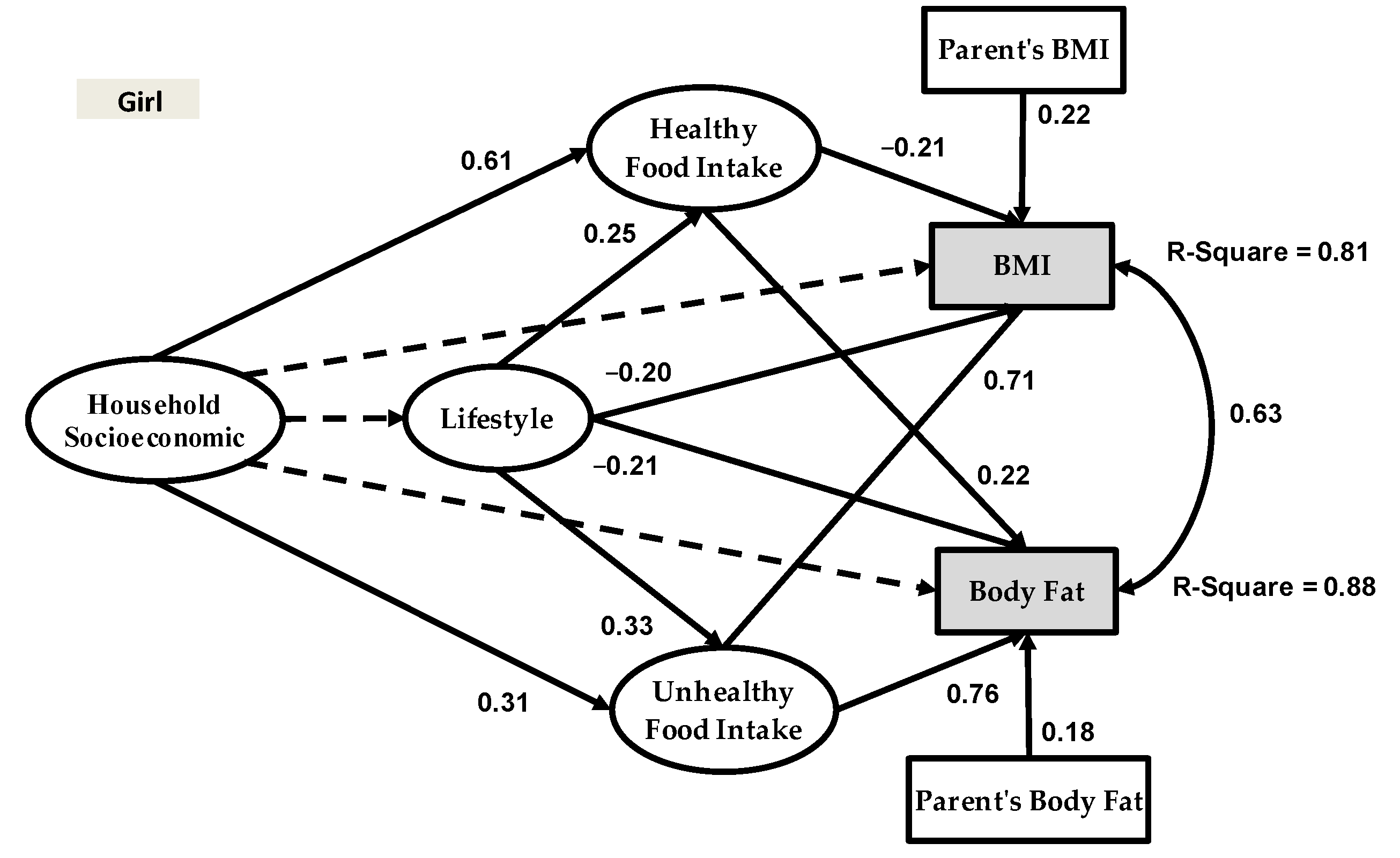
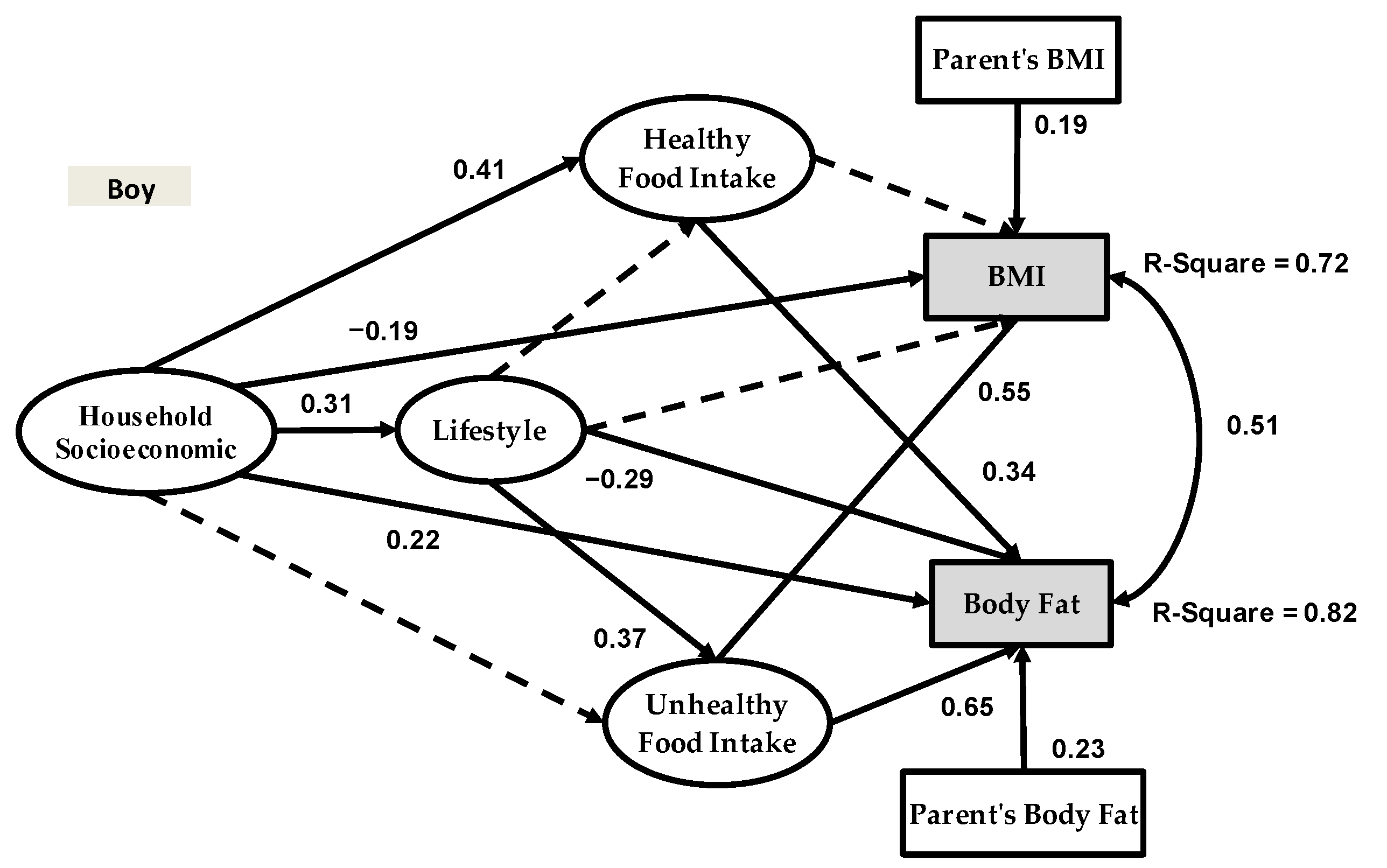
| Household Socioeconomic → Healthy Food Intake | 0.41 | 0.61 | 2.54 | 0.011 |
| Household Socioeconomic → Unhealthy Food Intake | 0.08 | 0.31 | 3.11 | 0.002 |
| Household Socioeconomic → Lifestyle | 0.31 | 0.05 | 3.36 | <0.001 |
| Household Socioeconomic → BMI | −0.19 | 0.10 | 4.06 | <0.001 |
| Household Socioeconomic → Body Fat | 0.22 | 0.09 | 1.88 | 0.060 |
| Lifestyle → Healthy Food Intake | 0.06 | 0.25 | 2.43 | 0.015 |
| Lifestyle → Unhealthy Food Intake | 0.37 | 0.33 | 0.45 | 0.652 |
| Lifestyle → BMI | −0.09 | −0.20 | 1.57 | 0.116 |
| Lifestyle → Body Fat | −0.29 | −0.21 | 1.04 | 0.298 |
| Healthy Food Intake → BMI | 0.09 | −0.21 | 4.23 | <0.001 |
| Healthy Food Intake → Body Fat | 0.34 | 0.22 | 1.65 | 0.098 |
| Unhealthy Food Intake → BMI | 0.53 | 0.71 | 2.22 | 0.026 |
| Unhealthy Food Intake → Body Fat | 0.65 | 0.76 | 1.57 | 0.116 |
| Parent’s BMI → BMI | 0.19 | 0.22 | 0.32 | 0.748 |
| Parent’s Body Fat → Body Fat | 0.23 | 0.18 | 0.76 | 0.447 |
Publisher’s Note: MDPI stays neutral with regard to jurisdictional claims in published maps and institutional affiliations. |
© 2021 by the authors. Licensee MDPI, Basel, Switzerland. This article is an open access article distributed under the terms and conditions of the Creative Commons Attribution (CC BY) license (https://creativecommons.org/licenses/by/4.0/).
Share and Cite
Salarzadeh Jenatabadi, H.; Shamsi, N.A.; Ng, B.-K.; Abdullah, N.A.; Mentri, K.A.C. Adolescent Obesity Modeling: A Framework of Socio-Economic Analysis on Public Health. Healthcare 2021, 9, 925. https://doi.org/10.3390/healthcare9080925
Salarzadeh Jenatabadi H, Shamsi NA, Ng B-K, Abdullah NA, Mentri KAC. Adolescent Obesity Modeling: A Framework of Socio-Economic Analysis on Public Health. Healthcare. 2021; 9(8):925. https://doi.org/10.3390/healthcare9080925
Chicago/Turabian StyleSalarzadeh Jenatabadi, Hashem, Nurulaini Abu Shamsi, Boon-Kwee Ng, Nor Aishah Abdullah, and Khairul Anam Che Mentri. 2021. "Adolescent Obesity Modeling: A Framework of Socio-Economic Analysis on Public Health" Healthcare 9, no. 8: 925. https://doi.org/10.3390/healthcare9080925